A 1.3 cm line survey toward Orion KL | Astronomy & Astrophysics (A&A)

Home

All issues

Volume 581 (September 2015)

A&A, 581 (2015) A48

Online Material

Free Access

Issue		A&A Volume 581, September 2015


Article Number		A48
Number of page(s)		60
Section		Interstellar and circumstellar matter
DOI		https://doi.org/10.1051/0004-6361/201526275
Published online		02 September 2015

Online material

Table 2

Lines detected in the survey of Orion-KL.

Table 4

Spatial origin of molecules detected by our 1.3 cm line survey.

Appendix A: The observed properties of detected lines in the survey

Table A.1

Transitions of recombination lines.

Table A.2

Observed properties of NH₃, ¹⁵NH₃ and NH₂D transitions.

Table A.3

Observed properties of CH₃OH transitions.

Table A.4

Observed properties of SO₂ and OCS transitions.

Table A.5

Observed properties of CH₃OCHO transitions.

Table A.6

Observed properties of H₂O, HDO, CH₃CN, HC₃N, HC₅N, CH₃OCH₃, H₂CO and HNCO transitions.

Appendix B: Zoom-in plots of observed spectra

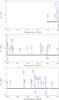	Fig. B.1 Observed spectrum of Orion KL from 17.9 to 26.2 GHz. The displayed frequency scale is based on the Local Standard of Rest velocity 0 km s^-1.
Open with DEXTER

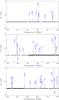	Fig. B.1 continued.
Open with DEXTER

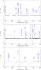	Fig. B.1 continued.
Open with DEXTER

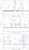	Fig. B.1 continued.
Open with DEXTER

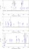	Fig. B.1 continued.
Open with DEXTER

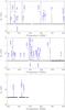	Fig. B.1 continued.
Open with DEXTER

	Fig. B.2 Observed Hα, Heα and Cα transitions indicated by dashed lines with n and Δn (see Sect. 4.1) also given. He63α is blended with H79β while He65α is blended with SO₂ (5_2,4 − 6_1,5). The velocity scale refers to the respective Hα line in each panel.
Open with DEXTER

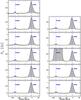	Fig. B.3 Observed Hβ and Heβ transitions indicated by dashed lines with n and Δn also given. H79β is blended with He63α while H81β is blended with NH₃ (3, 3). The velocity scale refers to the respective Hβ line in each panel.
Open with DEXTER

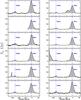	Fig. B.4 Observed Hγ and Heγ transitions indicated by dashed lines with n and Δn also given. The velocity scale refers to the respective Hγ line in each panel. The spectrum near He100γ is NH₃ (6,2).
Open with DEXTER

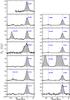	Fig. B.5 Observed Hδ and Heδ transitions indicated by dashed lines with n and Δn also given. The velocity scale refers to the respective Hδ line in each panel.
Open with DEXTER

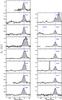	Fig. B.6 Observed Hε and Heε transitions indicated by dashed lines with n and Δn also given. The velocity scale refers to the respective Hε line in each panel.
Open with DEXTER

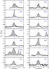	Fig. B.7 Observed Hζ transitions indicated by dashed lines with n and Δn also given. The velocity scale refers to the respective Hζ line in each panel.
Open with DEXTER

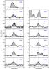	Fig. B.8 Observed Hη transitions indicated by dashed lines with n and Δn also given. The velocity scale refers to the respective Hη line in each panel.
Open with DEXTER

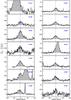	Fig. B.9 Observed Hθ transitions indicated by dashed lines with n and Δn also given. The velocity scale refers to the respective Hθ line in each panel.
Open with DEXTER

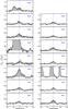	Fig. B.10 Observed Hι, Hκ and Hλ transitions indicated by dashed lines with n and Δn also given. The velocity scale refers to the respective Hι, Hκ and Hλ lines in each panel.
Open with DEXTER

	Fig. B.11 Observed NH₃ transitions with quantum numbers indicated in the upper right of each panel.
Open with DEXTER

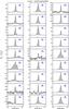	Fig. B.11 continued.
Open with DEXTER

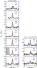	Fig. B.12 Observed ¹⁵NH₃ and NH₂D transitions with a one-component Gaussian fit shown (red lines). Quantum numbers are indicated in the upper right of each panel.
Open with DEXTER

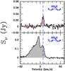	Fig. B.12 continued.
Open with DEXTER

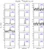	Fig. B.13 Observed CH₃OH and ¹³CH₃OH transitions with a one-component Gaussian fit shown (red lines). Species and quantum numbers are given in the upper right of each panel.
Open with DEXTER

	Fig. B.13 continued.
Open with DEXTER

	Fig. B.14 Observed SO₂ and OCS transitions (black lines) with a two- or three-component Gaussian fit shown together with the individual Gaussian components (red lines). Species and quantum numbers are given in the upper right of each panel. Note that SO₂ (5_2,4–6_1,5) is blended with He65α at 23 413.8 MHz and SO₂ (12_3,9–13_2,12) is blended with He107δ at 20 333.8 MHz.
Open with DEXTER

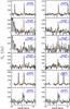	Fig. B.15 Observed CH₃OCHO transitions with one Gaussian fit shown (red lines). Species and quantum numbers are given in the upper right of each panel. In the CH₃OCHO (2_1,2–1_1,1 E) and CH₃OCHO (2_1,2–1_1,1 A) panels, the blue dashed lines represent the systemic velocities.
Open with DEXTER

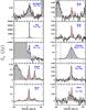Fig. B.16

Observed HC₃N, CH₃CN, HDO, H₂O, HNCO, H₂CO, CH₃OCH₃, HC₅N, and CH₃CH₂CN transitions. Species and quantum numbers are indicated in the upper right of each panel. For HC₃N, CH₃CN, HNCO, and CH₃CH₂CN, the spectra are fitted with the HFS method indicated by red lines. For the HDO and CH₃OCH₃ transitions which are blended, their systemic velocity is indicated by blue dashed lines.

Open with DEXTER

Appendix C: The ALMA maps of detected molecules and comparisons with other studies

We make use of the ALMA line survey archival data to study the distribution of molecules detected by our 1.3 cm line survey. The transitions used are listed in Table C.1. Figure C.1 shows the channel maps of these transitions. Note that the first [0,2] km s^-1 panel of NH₂D (3_2,2s − 3_1,2a) is contaminated by H₂CO (9_1,8 − 9_1,9) at 21 6268.7 MHz.

Recently, Feng et al. (2015) studied Orion KL using combined SMA and IRAM 30 m data, which covers parts of the frequency range of the ALMA-SV data. Here, we make a brief comparison between these data. By comparing the dust continuum emission in both datasets, mm2 in Feng et al. (2015) is resolved into MM4, MM5, and MM6 by ALMA. On the other hand, the dust continuum sources SR, NE, OF1N, and OF1S in Feng et al. (2015) are not detected in the ALMA-SV data. A comparsion of OCS (18–17) demonstrates that Feng et al. (2015) show more extended emission while the ALMA-SV data display more sub-structures. That is because the ALMA-SV data have a higher spatial resolution but lack short spacing and have a smaller primary beam.

We also estimate the flux loss by comparing the ALMA-SV data with those obtained with the IRAM-30 m single dish telescope. We make use of HC₃N (24–23) from Esplugues et al. (2013a), OCS (18–17) from Tercero et al. (2010), and SO₂ (11_5,7 − 12_4,8) from Esplugues et al. (2013b). Based on the telescope information¹⁰, we use a forward efficiency of 94%, a main

beam efficiency of 63%, and a conversion factor from brightness temperature to flux of 7.5 Jy/K to derive the total flux observed by the IRAM-30 m telescope. Meanwhile, the IRAM-30 m telescope has a spatial resolution of ~12′′, covering most emitting regions in Orion KL, so the IRAM-30 m data can be considered to represent the total flux densities of Orion KL. By integrating the whole regions of the ALMA-SV data, we find that the ALMA-SV data can account for 89% of the HC₃N (24–23), 57% of the OCS (18–17), and 44% of the SO₂ (11_5,7 − 4,8) emission.

Table C.1

Transitions from the ALMA line survey..

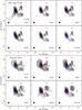Fig. C.1

Molecular line channel maps (contours) overlaid on the 230 GHz continuum map (grey). Grey shadings of the continuum image are 10%, 20%, 40%, 60%, 80% of the peak intensity of 1.406 Jy beam^-1. The contour levels of the molecular line images start at 5σ and continue in steps of 5σ, where the σ value for each transition is shown in the first panel in units of Jy beam^-1. The dotted contours are the negative features with the same contour absolute levels as the positive ones in each panel. The symbols are the same as in Fig. 1. The corresponding molecular transitions are indicated in the upper left of the first panel. The velocity range is given in the lower right of each panel in km s^-1. The synthesized beams of the molecular line images are shown in the lower left of each panel. The (0, 0) position in each panel is (α_J2000, δ_J2000) = (05^h35^m14.350^s, −05°22′35.00′′).

Open with DEXTER

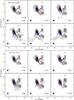	Fig. C.1 continued.
Open with DEXTER

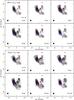	Fig. C.1 continued.
Open with DEXTER

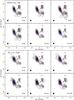	Fig. C.1 continued.
Open with DEXTER

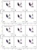	Fig. C.1 continued.
Open with DEXTER

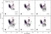	Fig. C.1 continued.
Open with DEXTER

© ESO, 2015

Current usage metrics show cumulative count of Article Views (full-text article views including HTML views, PDF and ePub downloads, according to the available data) and Abstracts Views on Vision4Press platform.

Data correspond to usage on the plateform after 2015. The current usage metrics is available 48-96 hours after online publication and is updated daily on week days.

Initial download of the metrics may take a while.