| Issue |
A&A
Volume 581, September 2015
|
|
|---|---|---|
| Article Number | A139 | |
| Number of page(s) | 22 | |
| Section | Extragalactic astronomy | |
| DOI | https://doi.org/10.1051/0004-6361/201525928 | |
| Published online | 24 September 2015 | |
Online material
Appendix A: Sketch of Balescu-Lenard derivation
Two derivations of the inhomogeneous Balescu-Lenard equation have been presented in the literature. The first one (Heyvaerts 2010) is based on the appropriate truncation at the order 1 /N of the BBGKY hierarchy. The second (Chavanis 2012a) relies on the Klimontovich equation, using a quasilinear approximation. We now briefly sketch the derivation presented in Chavanis (2012a). We consider an isolated system of N particles in interaction, of mass μ, in a physical space of dimension d. Their dynamics is entirely described by Hamilton’s equations  (A.1)where the Hamiltonian of the system is given by
  (A.2)Here u( | xi − xj |) is the binary potential of interaction. In the gravitational case, it satisfies u(x) = − G/ | x |. One can now introduce the discrete distribution function Fd(x,v,t) defined as
  (A.3)along with the corresponding potential
  (A.4)One can show that Fd satisfies the Klimontovich equation (Klimontovich 1967)
 ![]() (A.5)where we have defined the Hamiltonian Hd as
(A.5)where we have defined the Hamiltonian Hd as ![]() (A.6)At this stage, it is important to note that the Klimontovich Eq. (A.5)contains exactly the same information as Hamilton’s Eqs. (A.1). We now introduce the smooth distribution function F(x,v,t) = ⟨ Fd(x,v,t) ⟩, corresponding to an average of Fd over a large number of initial conditions. One can then write Fd = F + δF, where δF denotes fluctuations around the smooth distribution. In a similar way, we introduce ψ(x,v,t) = ⟨ ψd(x,v,t) ⟩, so that ψd = ψ + δψ. We have therefore decomposed the discrete distribution function Fd into a smooth component F that evolves slowly with time, whereas the fluctuating component δF evolves more rapidly. As a consequence, when considering the evolution of the fluctuations, one can assume the smooth distribution to be frozen. Using this timescale-decoupling approach, one can use the angle-action coordinates (θ1,J1) associated with the quasi-stationary smooth potential ψ to describe the fast evolution of the fluctuations. Using these decompositions and this change of coordinates, Eq. (A.5)takes the form of two evolution equations
(A.6)At this stage, it is important to note that the Klimontovich Eq. (A.5)contains exactly the same information as Hamilton’s Eqs. (A.1). We now introduce the smooth distribution function F(x,v,t) = ⟨ Fd(x,v,t) ⟩, corresponding to an average of Fd over a large number of initial conditions. One can then write Fd = F + δF, where δF denotes fluctuations around the smooth distribution. In a similar way, we introduce ψ(x,v,t) = ⟨ ψd(x,v,t) ⟩, so that ψd = ψ + δψ. We have therefore decomposed the discrete distribution function Fd into a smooth component F that evolves slowly with time, whereas the fluctuating component δF evolves more rapidly. As a consequence, when considering the evolution of the fluctuations, one can assume the smooth distribution to be frozen. Using this timescale-decoupling approach, one can use the angle-action coordinates (θ1,J1) associated with the quasi-stationary smooth potential ψ to describe the fast evolution of the fluctuations. Using these decompositions and this change of coordinates, Eq. (A.5)takes the form of two evolution equations  (A.7)and
  (A.8)where we have introduced the intrinsic frequencies of the system Ω1 = Ω(J1), as in Eq. (1), and where ⟨ . ⟩ denotes an angle average. Because of our timescale-decoupling approach, we may neglect the time variation of F(J1,t) in the calculation of the collision term (adiabatic approximation). It implies that F may be treated as a constant in Eq. (A.7)because F evolves on a (relaxation) timescale much larger than the (dynamical) time corresponding to the evolution of δF. In order to be valid, this approximation requires that N ≫ 1. Finally, we also assume that the distribution F remains Vlasov stable, so that its evolution is only governed by correlations and not by dynamical instabilities.
The first step of the derivation of the Balescu-Lenard equation is then to study the short timescale evolution Eq. (A.7). One defines the Fourier-Laplace transform of the fluctuation δF as  (A.9)valid for Im(ω1) sufficiently large. Similarly to Eq. (6), one also defines the spatial Fourier tranform of the initial value as
  (A.10)Thanks to these transformations, Eq. (A.7)may be rewritten under the form
  (A.11)We now use the basis elements introduced in Eq. (3), so that we may decompose the potential fluctuations under the form
  (A.12)We introduce the Laplace transform of ap(t) as
  (A.13)One can then take the inverse Fourier transform of Eq. (A.11), multiply by
 ![]() and integrate over θ1 and J1 (using the property that dxdv = dθ1dJ1). One gets
and integrate over θ1 and J1 (using the property that dxdv = dθ1dJ1). One gets  (A.14)where the response matrix
 ![]() is given by Eq. (5). Equation (A.14)can be rewritten under the form
is given by Eq. (5). Equation (A.14)can be rewritten under the form  (A.15)where the susceptibility coefficients have been introduced in Eq. (4). One can now compute the collision term appearing in the r.h.s. of Eq. (A.8). It requires us to evaluate
  (A.16)Using Eq. (A.11), one immediately obtains that
  (A.17)In Eq. (A.17), the first term corresponds to the self-correlation of the potential whereas the second term corresponds to the correlations between the potential fluctuations and the distribution function at time t = 0. Each of these terms must then be considered one at a time. Assuming that there is no correlation in the initial phases, one can show (see Appendix C from Chavanis 2012a) that
 ![]() (A.18)Hence, given Eq. (A.15), one can rewrite the first term of Eq. (A.17)under the form
(A.18)Hence, given Eq. (A.15), one can rewrite the first term of Eq. (A.17)under the form  (A.19)If we consider only the contributions that do not decay in time, one can perform the substitution
Starting from Eq. (A.19), thanks to the previous substitution and using the fact that ![]() , one can show that the first contribution from Eq. (A.16)takes the form
, one can show that the first contribution from Eq. (A.16)takes the form 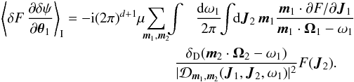 (A.20)The last step of the calculation is to use the Landau prescription ω → ω + i0+ along with Plemelj formula
 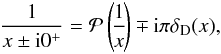 (A.21)where
 ![]() is the principal value. One can then rewrite Eq. (A.20)under the form
is the principal value. One can then rewrite Eq. (A.20)under the form 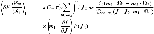 (A.22)Similarly, one can rewrite the second term of Eq. (A.17)under the form
  (A.23)Using symmetries of the matrix
 ![]() , starting from Eq. (A.23), one can show that the second contribution from Eq. (A.16)finally takes the form
, starting from Eq. (A.23), one can show that the second contribution from Eq. (A.16)finally takes the form  (A.24)Combining the two contributions obtained in Eqs. (A.22)and (A.24), one can rewrite Eq. (A.16)under the form
  (A.25)Hence, using the slow evolution Eq. (A.8), we recover the Balescu-Lenard equation introduced in Eq. (2). As a final remark, one may notice that on the short dynamical timescale, the evolution is governed by Eq. (A.7), which involves the fluctuating components δF and δψ of the distribution function and the potential. In contrast, on the long secular timescale, the evolution is governed by Eq. (A.8), which after an angle-average only involves the mean distribution function F. Indeed, thanks to the ensemble average, all the cross-correlations between the fluctuations δF and δψ, as in Eqs. (A.18), (A.19)and (A.23)can be expressed in terms of the underlying smooth distribution function F only, so that the fluctuating components are absent from the secular Balescu-Lenard collision operator from Eq. (A.25).
Appendix B: Turning off collective effects
The reference Chavanis (2013b; see also Appendix A of Chavanis 2012a) considers the inhomogeneous Balescu-Lenard equation without collective effects. This collisional kinetic equation is the equivalent of the Landau equation for inhomogeneous systems. It can be straightforwardly obtained as an approximation of the Balescu-Lenard Eq. (2). Indeed, one has to make the substitution from the dressed susceptibility coefficients ![]() to the bare ones given by Am1,m2(J1,J2), so that the inhomogeneous Balescu-Lenard equation without collective effects (i.e. the inhomogeneous Landau equation) is given by
to the bare ones given by Am1,m2(J1,J2), so that the inhomogeneous Balescu-Lenard equation without collective effects (i.e. the inhomogeneous Landau equation) is given by  (B.1)where the coefficients Am1,m2 are associated with the Fourier transform in angles of the interaction potential (Pichon 1994; Chavanis 2013b) and read
  (B.2)where u(x) is the binary potential of interaction given by u(x) = − G/ | x | in the gravitational case. A key remark at this stage is that the expression (B.2)does not require the introduction of biorthogonal basis elements as in Eq. (3), whereas in order to estimate the dressed susceptibility coefficients from Eq. (4), one must necessarily rely on Kalnajs’ matrix method (Kalnajs 1976). It is however possible to express Am1,m2 using the potential basis. Indeed, for a fixed value of x2, we consider the function x1 → u(x1 − x2). One can then decompose this function on the basis elements ψ(p)(x1), so that we may write
  (B.3)where it is important to note that the basis coefficients ap(x2) are functions of x2. Thanks to the biorthogonality property of the basis detailed in Eq. (3), one can obtain the expression of the coefficients ap(x2) which reads
  (B.4)where we used the fact that u is a real function. Hence we finally obtain
  (B.5)Taking appropriately a Fourier transform with respect to the angles as in Eq. (B.2), we obtain
  (B.6)This fairly simple relation allows us to express the bare susceptibility coefficients Am1,m2 using the potential basis. One does not need anymore to perform a Fourier transform in angles of the interaction potential because the resolution of Poisson’s equation has been implicitly hidden in the effective construction of the basis elements7. Neglecting the collective effects in the expression (4)of the dressed susceptibility coefficients amounts to taking
 ![]() , so that we obtain
, so that we obtain 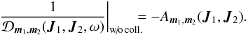 (B.7)The negative sign in Eq. (B.7)plays no significant role in the kinetic equations since one has to make the substitution of the square modulus
 ![]() in the Balescu-Lenard Eq. (2)to obtain the inhomogeneous Landau Eq. (B.1). Using our WKB basis, one can proceed similarly as in the dressed case, by limiting oneself only to local resonances. Equation (76)therefore becomes in the bare case
in the Balescu-Lenard Eq. (2)to obtain the inhomogeneous Landau Eq. (B.1). Using our WKB basis, one can proceed similarly as in the dressed case, by limiting oneself only to local resonances. Equation (76)therefore becomes in the bare case 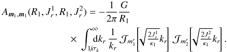 (B.8)This expression of the bare susceptibility coefficients can be straightforwardly obtained from the dressed ones by imposing λ = 0. One should note that because of the absence of the amplification term 1 / (1 − λkr), the approximation of the small denominators cannot be used. Hence a physically motivated evaluation of the expression (B.8)becomes more subtle to perform, especially because of the possibly important role that the Coulomb logarithm 1 /kr might play. Finally, one obtains that even for exactly local resonances, i.e. m1 = m2 and R1 = R2, the use of our WKB formalism allowed us to obtain non-diverging bare susceptibility coefficients. On the other hand, one could try to estimate the bare susceptibility coefficients starting from Eq. (B.2), i.e. without using any potential basis. Using the polar coordinates (R,φ), one has to compute
 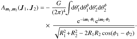 (B.9)By azimuthal symmetry, it is straightforward to show (Pichon & Cannon 1997) that
 ![]() (B.10)Hence the different mφ-modes of the Am1,m2 coefficients are independent. This result is identical to what was obtained in Eq. (65)for the dressed case. In order to illustrate the regularizing role of the WKB basis from Eq. (26), we will place ourselves in the context of an extremely tepid disc, and therefore assume
(B.10)Hence the different mφ-modes of the Am1,m2 coefficients are independent. This result is identical to what was obtained in Eq. (65)for the dressed case. In order to illustrate the regularizing role of the WKB basis from Eq. (26), we will place ourselves in the context of an extremely tepid disc, and therefore assume ![]() . Thanks to the epicyclic mapping from Eq. (24), one can drop all the dependences on θR appearing in R and φ. Equation (B.9)then immediately implies that
. Thanks to the epicyclic mapping from Eq. (24), one can drop all the dependences on θR appearing in R and φ. Equation (B.9)then immediately implies that ![]() (B.11)and the bare susceptibility coefficients are given by
(B.11)and the bare susceptibility coefficients are given by  (B.12)In this illustrative limit, we have by construction no contributions from the ILR and OLR resonances for which mr ≠ 0. After an immediate change of variables, using
 ![]() , it becomes
, it becomes 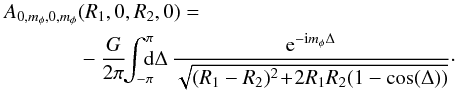 (B.13)The resonance condition from Eq. (68)takes the form mφΩφ(R1) = mφΩφ(R2) because we restricted ourselves in Eq. (B.11)to the case mr = 0. Hence assuming that the function Rg → Ωφ(Rg) is a monotonic function, one has to satisfy the constraint R1 = R2, so that we are restricting ourselves only to local resonances as in Eq. (72). For such resonances, Eq. (B.13)becomes
 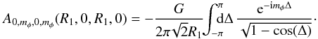 (B.14)At this stage, one must note that this integral is divergent. Indeed, for Δ → 0, one has
 ![]() . Hence the expression of the bare susceptibility coefficients derived from the Fourier transform of the interaction potential as in Eq. (B.2), when restricted to exactly local resonances becomes logarithmically divergent. This divergence, which is observed in the case of local resonances, is induced by the interaction of singular orbits. It is important to remark that this divergence was not present in Eq. (B.8)when computing the bare susceptibility coefficients using the WKB basis from Eq. (26). This implies that the WKB basis is not complete. For a complete biorthogonal basis, the expression (B.6)of the Am1,m2 coefficients is an exact expression. However, our calculation shows that the scale-decoupled WKB basis we used, possesses a subtle regularizing incompleteness which gets rid of the diverging contributions to the coefficients Am1,m2 in the limit of exactly local resonances.
. Hence the expression of the bare susceptibility coefficients derived from the Fourier transform of the interaction potential as in Eq. (B.2), when restricted to exactly local resonances becomes logarithmically divergent. This divergence, which is observed in the case of local resonances, is induced by the interaction of singular orbits. It is important to remark that this divergence was not present in Eq. (B.8)when computing the bare susceptibility coefficients using the WKB basis from Eq. (26). This implies that the WKB basis is not complete. For a complete biorthogonal basis, the expression (B.6)of the Am1,m2 coefficients is an exact expression. However, our calculation shows that the scale-decoupled WKB basis we used, possesses a subtle regularizing incompleteness which gets rid of the diverging contributions to the coefficients Am1,m2 in the limit of exactly local resonances.
Appendix C: The Schwarzschild DF case
When considering a Schwarzschild distribution function as in Eq. (25), while relying on the approximation of the small denominators from Eq. (78), one can explicitly perform the remaining integration on the radial action ![]() in the expressions (79)and (80)of the drift and diffusion coefficients. We now detail this explicit calculation. For such a Schwarzschild distribution function, it is straightforward to check that the gradients of the distribution function with respect to the actions are given by
in the expressions (79)and (80)of the drift and diffusion coefficients. We now detail this explicit calculation. For such a Schwarzschild distribution function, it is straightforward to check that the gradients of the distribution function with respect to the actions are given by  (C.1)Using the expression of the susceptibility coefficients from Eq. (78), after some simple algebra, one can rewrite the drift coefficients from Eq. (79)under the form
  (C.2)Similarly, the diffusion coefficients from Eq. (80)take the form
 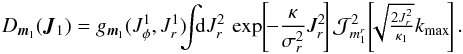 (C.3)In Eqs. (C.2)and (C.3), in order to shorten the notations, we introduced the function
 ![]() defined as
defined as 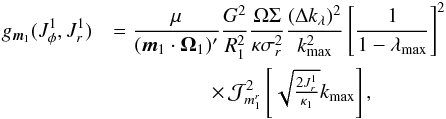 where we used the shortened notation
 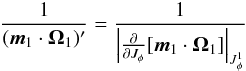 (C.4)for the term appearing as a prefactor in the expressions (79)and (80)of the drift and diffusion coefficients. In addition to the integration formula (57), we may also rely on the additional identity
  (C.5)where α> 0, β> 0, and mr ∈Z. In analogy with the definition from Eq. (58), we also introduce χmax as
 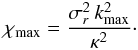 (C.6)One can then immediately perform the integration on
 ![]() from Eq. (C.3), so that the diffusion coefficients are given by
from Eq. (C.3), so that the diffusion coefficients are given by 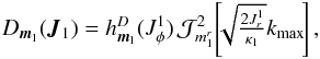 (C.7)where the function
 ![]() is defined as
is defined as 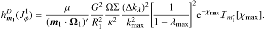 After some algebra, the drift coefficients from Eq. (C.2)are given by
 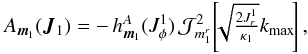 (C.8)where the function
 ![]() is defined as
is defined as 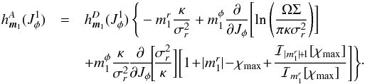 (C.9)These explicit expressions of the diffusion and drift coefficients obtained in Eqs. (C.7)and (C.8)allow us to estimate in a simple way the secular flux in the entire action space J = (Jφ,Jr), once we assume that the distribution function is a Schwarzschild DF given by Eq. (25)and that the susceptibility coefficients can be approximated by Eq. (78).
Appendix D: Relation to other kinetic equations
The kinetic equation governing the collisional evolution of a system of N stars at the order 1/N is the inhomogeneous Balescu-Lenard Eq. (2). This equation conserves the total number of stars and the energy, and monotonically increases the Boltzmann entropy (H-Theorem). We note that the collisional evolution of the system is due to a condition of resonance encapsulated in the term δD(m1·Ω1 − m2·Ω2). In general, this condition can allow for local and non-local resonances. In the case of tepid discs considered in the present paper, assuming that only tightly wound spirals are sustained by the disc, we justified in Eq. (72)the fact that the resonances are purely local, so that m1 = m2 and ![]() . Furthermore, because of the epicyclic approximation, the intrinsic frequencies of the system, given by Eq. (22), depend only on Jφ, so that Ω = Ω(Jφ). Under these conditions, the Balescu-Lenard equation giving the collisional evolution of F = F(Jφ,Jr,t) may be rewritten as
. Furthermore, because of the epicyclic approximation, the intrinsic frequencies of the system, given by Eq. (22), depend only on Jφ, so that Ω = Ω(Jφ). Under these conditions, the Balescu-Lenard equation giving the collisional evolution of F = F(Jφ,Jr,t) may be rewritten as 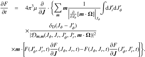 (D.1)The integration on
 ![]() is straightforward because of the δD-function (local resonance), and we are left with
is straightforward because of the δD-function (local resonance), and we are left with 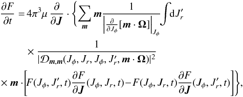 (D.2)where the susceptibility coefficients are generally given by Eq. (77).
The kinetic Eq. (D.2)is an integro-differential equation that governs the evolution of the system as a whole. It describes the effects of encounters between any test particle characterized by the angle-action coordinates (Jφ,Jr) and the field particles characterized by the (running) angle-action coordinates ![]() . Actually, there is no distinction between test and field particles, so that they are characterized by the same distribution function F(·,t) that evolves in a self-consistent manner, hence the integro-differential character of the kinetic equation. This is a characteristic of the Balescu-Lenard equation describing the evolution of the system as a whole.
. Actually, there is no distinction between test and field particles, so that they are characterized by the same distribution function F(·,t) that evolves in a self-consistent manner, hence the integro-differential character of the kinetic equation. This is a characteristic of the Balescu-Lenard equation describing the evolution of the system as a whole.
Appendix D.1: Fokker-Planck limit
We can also use this formalism to directly obtain the Fokker-Planck equation governing the relaxation of a test star in a bath of field stars, assumed to be in a steady state with a distribution function ![]() . Proceeding as in Chavanis (2012a), we just have to replace in Eq. (D.2)the distribution function of the field particles
. Proceeding as in Chavanis (2012a), we just have to replace in Eq. (D.2)the distribution function of the field particles ![]() by the static distribution
by the static distribution ![]() , while the time evolving distribution function of the test particle is rewritten as P(Jφ,Jr,t) for clarity. This heuristic procedure is justified in Chavanis (2012a) by an explicit calculation of the diffusion and drift coefficients of the Fokker-Planck equation. It transforms the integro-differential Eq. (D.2)into a differential equation
, while the time evolving distribution function of the test particle is rewritten as P(Jφ,Jr,t) for clarity. This heuristic procedure is justified in Chavanis (2012a) by an explicit calculation of the diffusion and drift coefficients of the Fokker-Planck equation. It transforms the integro-differential Eq. (D.2)into a differential equation 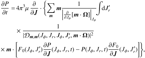 (D.3)which can be interpreted as a Fokker-Planck equation. If we assume that the field particles are at statistical equilibrium (thermal bath), described by the Boltzmann distribution
 ![]() (D.4)then, using the relation ∂F0/∂J = − βF0Ω (see the definition of Ω in Eq. (1)), we can reduce the Fokker-Planck Eq. (D.3)to the form
(D.4)then, using the relation ∂F0/∂J = − βF0Ω (see the definition of Ω in Eq. (1)), we can reduce the Fokker-Planck Eq. (D.3)to the form 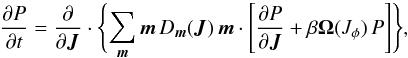 (D.5)with the diffusion coefficient
 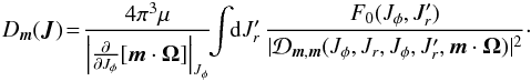 (D.6)We note that the friction term in the Fokker-Planck Eq. (D.5)is proportional and opposite to the intrinsic frequency Ω, and that the friction coefficient ξ satisfies a (generalized) Einstein relation ξ = Dβ (for each resonance) (Chavanis 2012a).
This Fokker-Planck formalism may have other applications. For example, if we consider a system with two species of particles (e.g. characterized by different masses mA and mB), and if species B has reached an equilibrium state with a distribution ![]() , we can use Eq. (D.3)to describe the relaxation of particles of species A due to the encounters with particles of species B (but neglecting the encounters between particles of species A). This approach is further discussed in Appendix F of Chavanis (2013b). On the other hand, for a single species system, we may describe the early dynamics of the system as a whole with a good approximation by replacing
, we can use Eq. (D.3)to describe the relaxation of particles of species A due to the encounters with particles of species B (but neglecting the encounters between particles of species A). This approach is further discussed in Appendix F of Chavanis (2013b). On the other hand, for a single species system, we may describe the early dynamics of the system as a whole with a good approximation by replacing ![]() in the Balescu-Lenard Eq. (D.2)by the initial distribution function
in the Balescu-Lenard Eq. (D.2)by the initial distribution function ![]() , leading again to an equation of the form (D.3).
, leading again to an equation of the form (D.3).
Appendix D.2: Other kinetic equations
We now compare the previous results to other related kinetic equations. For spatially homogeneous systems with long-range interactions, the Balescu-Lenard equation reads (see Chavanis 2012c):  (D.7)where
  (D.8)is the dielectric function. For one-dimensional systems, it reduces to the trivial form
 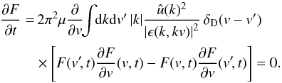 (D.9)In d> 1, there are always resonances between particles with different velocities, implying that the Balescu-Lenard equation relaxes towards the Boltzmann distribution on a timescale of the order NtD, where tD is the dynamical time. By contrast, in d = 1, the resonances become local (in velocity space) and since the term in brackets is anti-symmetric with respect to the interchange of v and v′, the Balescu-Lenard diffusion current vanishes exactly. This implies that the relaxation time is larger than NtD, presumably of the order N2tD, corresponding to the next order term in the expansion of the dynamics in powers of 1 /N. The Fokker-Planck equation describing the evolution of a test particle in a bath of field particles is discussed in Chavanis (2012c, 2013a).
The kinetic equation governing the collisional evolution of a system of N point vortices in two-dimensional hydrodynamics at the order 1 /N can be written, in the axisymmetric case, as (see Chavanis 2012b): 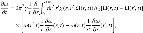 (D.10)where ω(r,t) is the profile of vorticity, Ω(r,t) the profile of angular velocity, and χ(r,r′,Ω(r,t)) is related to the dressed potential of interaction between the point vortices (see Chavanis 2012b for more details). This equation conserves the total number of point vortices and the energy, and monotonically increases the Boltzmann entropy (H-theorem). If the profile of angular velocity is monotonic, the kinetic equation reduces to the form
 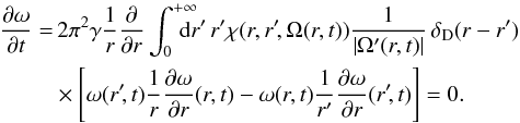 (D.11)For non-monotonic profile of angular velocity, one can have non-local resonances (i.e. distant collisions between point vortices), as studied in Chavanis & Lemou (2007). This produces a diffusion current. If the profile of angular velocity is, or becomes, monotonic, the resonances are purely local and, since the term in brackets is anti-symmetric with respect to the interchange of r and r′, the diffusion current also vanishes. This implies that the relaxation time is larger than NtD as discussed above. The Fokker-Planck equation describing the evolution of a test vortex in a sea of field vortices is discussed in Chavanis (2012b).
If we focus on purely local resonances, we note that the inhomogeneous Balescu-Lenard Eq. (D.1)is different from Eqs. (D.9)and (D.11)because it is two-dimensional in Jr and Jφ, and the resonances act only on Jφ. Therefore, purely local resonances do not yield a zero flux, contrary to Eqs. (D.9)and (D.11). This really is an effect of the two-dimensionality of the system. Indeed, for local resonances, the 1D inhomogeneous equation also yields a zero flux: 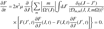 (D.12)
Appendix E: The Schwarzschild conspiracy
The Schwarzschild distribution function introduced in Eq. (25)and considered in S12 simulation has the specificity to be exponential in the Jr-direction, so that F is Boltzmannian with respect to the Jr variable. It is known (e.g. Chavanis 2012a) that the (complete) Boltzmann distribution is the steady state of the Balescu-Lenard Eq. (2). Therefore, we can expect that the (partial) exponential behaviour of the Schwarzschild distribution will induce simplifications that we now detail. In analogy with Eq. (10), the flux associated with a given resonance m is defined as 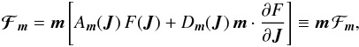 (E.1)where the non-bold ℱm is a scalar. Using shortened notations and forgetting numerical prefactors, we may rewrite the drift and diffusion coefficients from Eqs. (79)and (80)under the form
 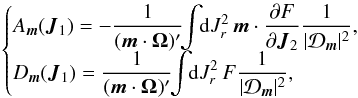 (E.2)where we used the same shortened notation for the resonant factor 1 / (m·Ω)′ as in Eq. (C.4). The flux can then be decomposed as
 ![]() with
with  (E.3)and
 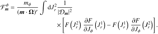 (E.4)We are interested in the value of the flux at the initial time, where the distribution function is given by the Schwarzschild distribution. Because of the exponential dependence in Jr of the Schwarzschild distribution function, one has
 ![]() . As a result, the radial component (E.3)of the flux cancels out and the flux is simply given by Eq. (E.4). This coincidence could be called the Schwarzschild conspiracy and has important consequences on the properties of the collisional diffusion. Indeed, for a tepid disc, one has | ∂F/∂Jr | ≫ | ∂F/∂Jφ |. Hence one would expect the gradients with respect to Jr to be the major contributors to the diffusion. When considering independently the drift and diffusion coefficients, the gradients in ∂F/∂Jr dominate the diffusion current. Thus for mr ≠ 0, the diffusion-only flux can be approximated by
. As a result, the radial component (E.3)of the flux cancels out and the flux is simply given by Eq. (E.4). This coincidence could be called the Schwarzschild conspiracy and has important consequences on the properties of the collisional diffusion. Indeed, for a tepid disc, one has | ∂F/∂Jr | ≫ | ∂F/∂Jφ |. Hence one would expect the gradients with respect to Jr to be the major contributors to the diffusion. When considering independently the drift and diffusion coefficients, the gradients in ∂F/∂Jr dominate the diffusion current. Thus for mr ≠ 0, the diffusion-only flux can be approximated by 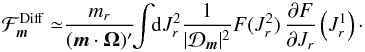 (E.5)As the ILR and the OLR have a non-zero mr compared to the COR, these resonances should dominate independently the drift and diffusion components. However, when considering the full flux made of the contributions from the drift and diffusion coefficients, because of the Schwarzschild conspiracy, there is a simplification of the dominant terms in ∂F/∂Jr, so that one recovers as in Eq. (E.4)that only the smaller gradients ∂F/∂Jφ remain present. The Schwarzschild conspiracy between drift and diffusion will therefore tend to slightly reduce the magnitude of the full diffusion flux, so as to moderately slow down the collisional relaxation. More importantly, the Schwarzschild conspiracy will favour the COR resonance (radial migration) over the ILR resonance (Jr-heating). One should note that the DF which is effectively sampled in S12 is of the form
 ![]() , with
, with ![]() (Toomre 1977; Binney & Tremaine 2008). It is only within the epicyclic approximation that this DF takes the form of the Schwarzschild DF from Eq. (25). As a consequence, in S12 simulation, the Schwarzschild conspiracy is not exactly satisfied as observed in Eq. (E.3), but the residual difference driving the secular diffusion is likely to be subdominant, as illustrated in Fig. E.1.
(Toomre 1977; Binney & Tremaine 2008). It is only within the epicyclic approximation that this DF takes the form of the Schwarzschild DF from Eq. (25). As a consequence, in S12 simulation, the Schwarzschild conspiracy is not exactly satisfied as observed in Eq. (E.3), but the residual difference driving the secular diffusion is likely to be subdominant, as illustrated in Fig. E.1.
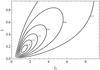 |
Fig. E.1
Contours in action-space (Jφ,Jr) of the difference between the sampled anisotropic DF of S12 simulation |
| Open with DEXTER | |
Appendix F: Temporal frequency selection
An important feature of the diffusion Eq. (7)is that the diffusion takes place along specific resonance directions associated with the vectors m as discussed in Eq. (16). Hence being able to determine the dominant resonance is crucial in order to estimate the direction of the secular diffusion in action space. The temporal frequency associated with a given resonance m in a location J of action-space is given by ω = m·Ω. Thanks to the expression (83), one immediately obtains that for a Mestel disc, one has ![]() (F.1)In Fouvry & Pichon (2015), Fouvry et al. (2015a), we studied the same S12 simulation using the WKB limit of the secular diffusion equation, which intends to describe the secular forcing of a collisionless self-gravitating system perturbed by an external source. An essential assumption of this approach was to consider the external perturbation as originating from numerical Poisson shot noise, and therefore assume it to be proportional to the local active surface density. The autocorrelation of the external perturbation ψext was taken to be equal to
(F.1)In Fouvry & Pichon (2015), Fouvry et al. (2015a), we studied the same S12 simulation using the WKB limit of the secular diffusion equation, which intends to describe the secular forcing of a collisionless self-gravitating system perturbed by an external source. An essential assumption of this approach was to consider the external perturbation as originating from numerical Poisson shot noise, and therefore assume it to be proportional to the local active surface density. The autocorrelation of the external perturbation ψext was taken to be equal to ![]() (F.2)One can remark that this crude assumption on the noise properties has no ω dependence, so that all resonances are equally favoured by the Poisson shot noise and are perturbed similarly whatever their associated intrinsic frequencies ω = m·Ω. This ad hoc and simple noise approximation is one of the limitations of the formalism presented in Fouvry & Pichon (2015), Fouvry et al. (2015a). In contrast, in the WKB Balescu-Lenard equation described in this paper, this preferential selection of the resonances based on their intrinsic frequency is naturally present. Indeed, one can note in the expression (E.4)of the flux associated with a resonance m, the presence of the prefactor 1 / (m·Ω)′
(F.2)One can remark that this crude assumption on the noise properties has no ω dependence, so that all resonances are equally favoured by the Poisson shot noise and are perturbed similarly whatever their associated intrinsic frequencies ω = m·Ω. This ad hoc and simple noise approximation is one of the limitations of the formalism presented in Fouvry & Pichon (2015), Fouvry et al. (2015a). In contrast, in the WKB Balescu-Lenard equation described in this paper, this preferential selection of the resonances based on their intrinsic frequency is naturally present. Indeed, one can note in the expression (E.4)of the flux associated with a resonance m, the presence of the prefactor 1 / (m·Ω)′
which arose in Eq. (67)when handling the resonance condition. For the Mestel disc, whose intrinsic frequencies are given by Eq. (83), this term can be straightforwardly computed and reads 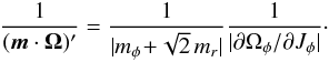 (F.3)Comparing the ILR resonance to the OLR and COR, one immediately obtains that
 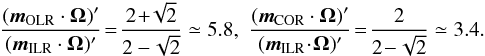 (F.4)Hence because the ILR resonance is associated with lower intrinsic temporal frequency ω = m·Ω, the resonant factor 1 / (m·Ω)′ naturally tends to favour the ILR resonance with respect to the OLR and COR, and therefore performs natively a temporal frequency biasing which was absent from the ad hoc assumption of Eq. (F.2)describing the external forcing considered in Fouvry & Pichon (2015), Fouvry et al. (2015a).
One can even be more specific when comparing the ILR and OLR resonances. The only difference between these two resonances is the sign of mr. The expression (62)of the amplification eigenvalues shows that its value only depends on s2, so that λILR = λOLR. The expression of the susceptibility coefficients from Eq. (77)is also independent of the sign of mr so that ![]() . Hence, when considering the flux ℱm given by Eq. (E.4), one notes that between the ILR and OLR resonances, ℱm only changes through the factor 1 / (m·Ω)′. Thanks to Eq. (F.4), one immediately obtains
. Hence, when considering the flux ℱm given by Eq. (E.4), one notes that between the ILR and OLR resonances, ℱm only changes through the factor 1 / (m·Ω)′. Thanks to Eq. (F.4), one immediately obtains 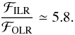 (F.5)The secular diffusion flux associated with the OLR resonance is therefore always much smaller than the one associated with the ILR resonance because of this effect of temporal frequency biasing.
As a conclusion, the temporal frequency selection effect described in Eq. (F.4)will tend to favour the ILR resonance because it is associated with a smaller intrinsic frequency. However, one can observe in Fig. 8 that the COR resonance is always more amplified than the ILR resonance. Finally, the crucial remark is to note that the susceptibility coefficients from Eq. (77)involve Bessel functions ![]() , which are such that
, which are such that ![]() if mr = 0, or = 0 otherwise. As a consequence, close to the Jr = 0 axis, the COR resonance will always tend to become the dominant resonance. There is therefore a non-trivial arbitration between these opposite effects when considering the respective contributions of the various resonances to the full secular diffusion flux.
if mr = 0, or = 0 otherwise. As a consequence, close to the Jr = 0 axis, the COR resonance will always tend to become the dominant resonance. There is therefore a non-trivial arbitration between these opposite effects when considering the respective contributions of the various resonances to the full secular diffusion flux.
© ESO, 2015
Current usage metrics show cumulative count of Article Views (full-text article views including HTML views, PDF and ePub downloads, according to the available data) and Abstracts Views on Vision4Press platform.
Data correspond to usage on the plateform after 2015. The current usage metrics is available 48-96 hours after online publication and is updated daily on week days.
Initial download of the metrics may take a while.