| Issue |
A&A
Volume 580, August 2015
|
|
|---|---|---|
| Article Number | A13 | |
| Number of page(s) | 27 | |
| Section | Galactic structure, stellar clusters and populations | |
| DOI | https://doi.org/10.1051/0004-6361/201424434 | |
| Published online | 20 July 2015 | |
Online material
Appendix A: Validation of FastMEM
Appendix A.1: Reconstruction of the free-free component using FastMEM
The Maximum Entropy Method (MEM) is used to separate the signals from cosmological and astrophysical foregrounds including CMB and Galactic foregrounds such as synchrotron, free-free, anomalous microwave emission (AME) and thermal dust. The implementation of MEM used here works in the spherical harmonic domain, where the separation is performed mode-by-mode allowing a huge optimization problem to be split into a number of smaller problems that can be done in parallel, saving CPU time. This approach, called FastMEM, is described by Hobson et al. (1998) for Fourier modes on flat patches of the sky and by Stolyarov et al. (2002) for the full-sky case.
The simulated data set used to check the quality of the recovery and reconstruction errors was the Full Focal Plane data set FFP4 (Planck Collaboration 2013). It includes all Planck frequency maps from 30 to 857 GHz properly simulated with plausible noise levels, systematics due to the scanning strategy, and real beam transfer functions. The components were modelled using the Planck Sky Model (PSM; Delabrouille et al. 2013) v1.7.
After multiple separation tests it was found that low-frequency components are very complicated to extract, especially AME. It was decided to use only the limited number of frequency maps, from 70.4 to 353 GHz. Since there were problems with WMAP modelled maps, they were not used in the analysis. However, WMAP data maps are essential for low-frequency component extraction from the real data.
The reconstructed components were CMB, thermal SZ, free-free, thermal dust, and CO J = 1 →0, J = 2 → 1 and J = 3 → 2 lines. It was assumed that AME and synchrotron contributions are very small in this range of frequencies. A small bias from the synchrotron component, however, could be possible in the Galactic plane. Free-free spectral scaling was calculated assuming average electron temperature Te = 6000 K (Alves et al. 2012).
The accuracy of the component separation was controlled in several ways. Firstly, the
residuals between data maps and the modelled component contribution were calculated.
There were component-free maps, containing only instrumental noise and point sources
![]() (A.1)and component-cleaned CMB maps at each
frequency, containing CMB signal as well as receiver noise and point sources
(A.1)and component-cleaned CMB maps at each
frequency, containing CMB signal as well as receiver noise and point sources
![]() (A.2)To calculate residual maps one should
smooth component models with the same beam, which is taken to be a Gaussian with
(A.2)To calculate residual maps one should
smooth component models with the same beam, which is taken to be a Gaussian with
![]() at 70.4 GHz. Residual maps are
shown on the Fig. A.1.
at 70.4 GHz. Residual maps are
shown on the Fig. A.1.
The reconstructed free-free map can be directly compared with the input template. The residual map shows that the reconstruction slightly overestimates the real free-free contribution in the Galactic plane (Fig. A.2), where the morphology is complex and includes many bright point sources.
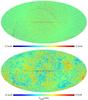 |
Fig. A.1
Simulated data: residual maps at 70.4 GHz, containing only receiver noise and point sources (Eq. (A.1), upper panel) and CMB component-cleaned map (Eq. (A.2), lower panel). The maps are in Mollweide projection, with Nside = 1024 and a linear temperature scale with units of TCMB. |
| Open with DEXTER | |
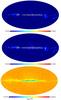 |
Fig. A.2
Input, reconstructed and residual maps of the free-free emission at 70.4 GHz. All maps are in Mollweide projection, smoothed with a 1° beam, Nside = 128. The colour scale is linear, and the units are mKCMB. |
| Open with DEXTER | |
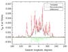 |
Fig. A.3
Input, reconstructed and residual Galactic plane profiles for the free-free emission at 70.4 GHz. Profiles were calculated over the maps shown in Fig. A.2; units are KCMB. The plots are made for a 1°-resolution cut along the Galactic plane. |
| Open with DEXTER | |
It is also useful to consider the profiles of free-free emission along the Galactic plane, which are shown on the Fig. A.3, and T–T plots between input and reconstructed maps (Fig. A.4).
Appendix A.2: Comparison of free-free maps from FastMEM with other component separation methods
In this section we compare the free-free emission derived from FastMEM and other modelling methods with the direct measure of free-free using RRLs. In order to convert the RRL data to brightness temperature we have used an electron temperature, Te, of 6000 K as found by Alves et al. (2012) for the Galactic plane region l = 20°–44°, | b | ≤ 4°, which we also use for this comparison.
FastMEM was applied to Planck data in the frequency range 70.4−353 GHz and used to obtain the free-free, CO, and thermal dust components. The synchrotron component was assumed to be a small fraction of the total Galactic plane emission at these frequencies. This was tested by subtracting the synchrotron component found by Alves et al. (2012) with brightness temperature spectral indices in the range βsynch = −2.7 to −3.1; the free-free component changed by ≤2%. Similarly, the effect of the AME component was minimal in the 70.4−353 GHz range. The AME amplitude was based on the 100 μm IRIS brightness and assuming 10 μK per MJy sr-1 at 30 GHz with a spectrum peaking at 20 GHz.
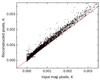 |
Fig. A.4
T–T plot comparing the pixel values in the simulated input map and in the reconstructed map. The solid red line indicates equality. The frequency is 70.4 GHz and the temperature scale is KCMB. |
| Open with DEXTER | |
The WMAP 9-yr MEM free-free all-sky fit (Bennett et al. 2013) was used to map the l = 20°–44°, | b | ≤ 4° region of the Alves et al. (2012) RRL survey, which includes emission from the Sagittarius and Scutum spiral arms of the inner Galaxy. This fit is based on the WMAP frequency range 23−94 GHz and includes significant synchrotron and AME emission that could also be estimated separately.
The Correlated Component Analysis (CCA) component separation method (Bonaldi et al. 2006), as used in Planck Collaboration Int. XII (2013), was also applied to the RRL region. The map of the free-free from RRLs is compared with those from FastMEM, WMAP9 MEM and CCA in Fig. A.5. The two MEM models and CCA are remarkably similar. The RRLs show the same structure but are somewhat weaker as we now show.
|
Fig. A.5
Maps of the l = 20°–44°, b = −4°–+ 4° region of the inner Galaxy showing the free-free emission derived from RRLs, FastMEM, WMAP9 MEM, and CCA. The maps are at 33 GHz with 1° resolution and Nside = 128. The colour-coding is on a linear scale running from −1 to 10 mKRJ. |
|
| Open with DEXTER | |
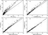 |
Fig. A.6
T–T plots comparing the free-free estimates from RRLs, WMAP9 MEM, and Planck data using FastMEM and CCA. The lower line indicates equality while the other line (where present) indicates the best fit. The frequency is 33 GHz and the resolution is 1°, with Nside = 128. |
| Open with DEXTER | |
The T–T plots in Fig. A.6 show the relationships between the amplitudes of the RRL measurements
and the three models. It can be seen that FastMEM from Planck and
WMAP9 MEM agree closely. The CCA amplitudes are somewhat larger than the MEM
solutions. The corresponding RRL amplitudes calculated for Te = 6000 K
are lower by ~30%.
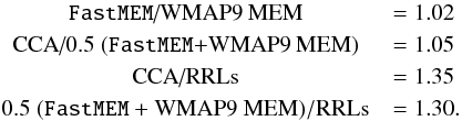
The best fitting ratios of the slopes after removing offsets and including the
brighter data only (Tb ≥ 0.3 mK) are:
We now consider what systematics could account for the difference between the RRL measurement and the three models, all of which agree within ~5%. The assumption of Te = 6000 K for the RRLs could be the source of part of the 30% difference. An increase of Te from 6000 K to 7000 K for example would increase the free-free brightness temperature by 19%. On the other hand, the three models considered here each need to take account of the other foregrounds, which they do in different ways. This could possibly lead to an overestimate of the free-free emission if the other three spectral components were underestimates. We suggest that this difference may be resolved by using Te = 7000 K and reducing the free-free component map by 10%.
© ESO, 2015
Current usage metrics show cumulative count of Article Views (full-text article views including HTML views, PDF and ePub downloads, according to the available data) and Abstracts Views on Vision4Press platform.
Data correspond to usage on the plateform after 2015. The current usage metrics is available 48-96 hours after online publication and is updated daily on week days.
Initial download of the metrics may take a while.