| Issue |
A&A
Volume 580, August 2015
|
|
|---|---|---|
| Article Number | A80 | |
| Number of page(s) | 17 | |
| Section | The Sun | |
| DOI | https://doi.org/10.1051/0004-6361/201424397 | |
| Published online | 06 August 2015 | |
Online material
Appendix A: Calculation of energy density of energetic protons
Here we investigate the contribution of the energetic particles to the total energy content of the plasma by calculating the energy density of a major SEP event at 1 AU and by comparing it with the energy density of the local magnetic field. In the case where the computed energy density of the energetic protons (ϵp) at 1 AU exceeds the local magnetic field energy density (ϵB), the particles are no longer confined into magnetic flux tubes and they can modulate the local magnetic field. The proton energy density can be derived from the following equations:  (A.1)where E is the particle energy, Ω is the instrument solid angle, and β is the particle velocity in υ/ c. The integration over the angle Ω is calculated for the particle detector effective angle (field of view) and the integration over the energy is calculated from the minimum (E1) to the maximum (E2) energy of the detected protons. The magnetic energy density is given by the following equation:
  (A.2)In the above equation, the magnitude of the magnetic field is measured in Tesla and the magnetic energy density is in Joules/m3.
We selected the SEP event of 26 December 2001 to analyse. To derive proton spectra, we used the SOHO/ERNE particle data of one minute average values. The SOHO/ERNEs’ particle detectors field of view (half angle; Torsti et al. 1995) is ~30° for the low-energy detector (LED) and ~60° for the high-energy detector (HED). Combining the data of the HED and the LED, we have an energy coverage from 1.68 to 108 MeV. We first estimated the SEP energy spectra and then we integrated E dN/ dE to derive the ϵp. For the calculation of the energy spectra, we chose not to perform a time shift between the different energy channels because we wanted to compare ϵp with the measurements of the local magnetic field, at 1 AU and not at the acceleration site. For the computation of the ϵB, we used one minute average data from Wind Magnetic Field Investigation (MFI) instrument, for the magnitude of the average magnetic field vector.
In Fig. A.1 we present the proton intensity and the magnitude of the magnetic field for the event of 26 December 2001. At 12:10 UT we calculated the proton energy spectra (blue line) and the measure of E2 dN/ dE (green line). The latter in logarithmic scale is proportional to the integral in Eq. (A.1) and its value shows the energy region where the contribution to the integral is maximum; in our case the maximum contribution to the proton energy density comes from protons with energy close to 10 MeV. The magnetic energy density was ϵB = 2.6 × 10⁻¹¹ J/m3 and this value is almost three orders of magnitude larger than the calculated proton energy density whose value was ϵp = 3.8 × 10⁻¹⁴ J/m3.
From the above analysis, it is evident that the magnetic energy density for the 26 December 2001 event is much larger than the non-thermal proton energy density. We repeated the same analysis for the very energetic events (Ip> 0.2 pfu) of 26 October and 02 November of 2003 and we found similar results; the lowest difference between ϵB and ϵp was almost two orders of magnitude.
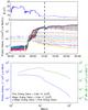 |
Fig. A.1
Data for the calculation of the proton and magnetic energy density for the SEP event of 26 December 2001 at 12:10 UT. Top: average of the magnetic field vector from Wind/IMF. Middle: proton intensity in 20 energy channels of SOHO/ERNE. The vertical black dash-dotted line marks the time of the energy density calculation. Bottom: proton energy spectrum in logarithmic scale at 12:10 UT shown with a blue line and the measure of E2dN/ dE shown with a green line. |
| Open with DEXTER | |
Appendix B: Table of events with inferred radio association
In Table B.1 we present our results for the 65 proton events with “inferred radio association”. In Cols. 2 and 3 we give the proton release times and path lengths, respectively, with their uncertainties as inferred from the VDA. Also, in Col. 4 we give for every event the resulting transient radio emission associated with the proton release according to the analysis of Sect. 3. In Col. 5 we present the locations of their associated flares that were used in the analysis of Sect. 4. The “–” entries correspond to flares occurred far behind the west limb. The electron release times and path lengths with their uncertainties as inferred by the VDA of Sect. 5.2 are given in Cols. 6 and 7, respectively. The estimated start times of the type III bursts used in the relative timings of Sect. 5.1 are presented in Col. 8.
Events with “inferred radio association”.
© ESO, 2015
Current usage metrics show cumulative count of Article Views (full-text article views including HTML views, PDF and ePub downloads, according to the available data) and Abstracts Views on Vision4Press platform.
Data correspond to usage on the plateform after 2015. The current usage metrics is available 48-96 hours after online publication and is updated daily on week days.
Initial download of the metrics may take a while.