| Issue |
A&A
Volume 579, July 2015
|
|
|---|---|---|
| Article Number | A104 | |
| Number of page(s) | 12 | |
| Section | Galactic structure, stellar clusters and populations | |
| DOI | https://doi.org/10.1051/0004-6361/201425509 | |
| Published online | 08 July 2015 | |
Online material
Appendix A: Line-by-line MyGIsFOS fits
MyGIsFOS operates by fitting a region around each relevant spectral line against a grid of synthetic spectra, and deriving the best-fitting abundance directly, rather than using the line equivalent width (EW), which MyGIsFOS computes, but mainly to estimate Vturb. While this makes MyGIsFOS arguably more robust against the effect of line blends, it makes it rather pointless to provide a line-by-line table of EWs, atomic data, and derived abundances, unless atomic data for all the features included in the fitted region are provided, which is quite cumbersome.
To allow verification and comparison of our results, we thus decided to provide the per-feature abundances as well as the actual observed and synthetic best-fitting profile for each fitted region. We describe here in detail how these results will be delivered, since we plan to maintain the same format for any future MyGIsFOS-based analysis.
The ultimate purpose of these comparisons is to ascertain whether abundance differences between works stem from any aspect of the line modeling, and assess the amount of the effect. We believe that providing the observed and synthetic profiles is particularly effective in this sense for a number of reasons:
-
The reader can apply whatever abundance analysis techniquehe/she prefers to either the observed or the synthetic spectra. Forinstance, if EWs are employed, he/she can determine the EW ofeither profile, and derive the abundance with his/her choice ofatomic data, atmosphere models, and so on. This would allowhim/her to directly determine what abundance the chosenmethod would assign to our best-fitting synthetic, and to compareit with the one we derive.
-
The reader can evaluate whether our choice of continuum placement corresponds or differs from the one he/she applied, and assess the broadening we applied to the syntheses, both looking at the feature of interest, and looking for any other useful feature (e.g. unblended Fe i lines, which are often used to set the broadening for lines needing synthesis).
-
The reader can directly assess the goodness of our fit with whatever estimator he/she prefers.
-
The reader gains access to the actual observed data we employed for every spectral region we used. Not every spectrum is available in public archives, and even fewer are available in reduced, and (possibly) coadded form.
An example of MyGIsFOS fit results is presented in Fig. A.1. To make the results easy to handle by Vizier, they were split into two tables:
-
The features table contains basic data for each regionsuccessfully fitted in every star. This includes a code identifyingthe star (e.g. N5053_69), the ion the feature was used to measure,the starting and ending wavelength, the derived abundance, theEWs for the observed and best-fitting synthetic (determined byintegration under the pseudo-continuum), the local S/N, the small Doppler and continuum shift that MyGIsFOS allows in the fitting of each feature, flags to identify the Fe i features that were used in the Teff and Vturb fitting process (the flags are not relevant for features not measuring Fe i), and finally a feature code formed of the element, ion, and central wavelength of the fitted range (e.g. 3000_481047). This last code is unique to each feature, and it can be used to retrieve the profile of the fit from the next table.
-
The fits table contains all the fitted profiles for all the features for all the stars. Each line of the table corresponds to a specific pixel of a specific fit of a specific star, and contains the star identifying code, then the feature identifying code, followed by the wavelength, and the (pseudonormalized) synthetic and observed flux in that pixel. The user interested, for instance, in looking at the fit of the aforementioned Zn i feature in star NGC 5053-69, has simply to select from the table all the lines beginning with “N5053_69 3000_481047”.
Both tables are available through CDS. To reproduce the fit as plotted in Fig. A.1, the synthetic flux must be divided by the continuum value provided in the features table.
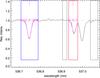 |
Fig. A.1
An example of MyGIsFOS fit for two features of star NGC 5634-2. The blue box corresponds to a Fe i feature, while the red box is a Co i feature. Gray boxes are pseudo-continuum estimation intervals. Observed pseudo-normalized spectrum is in black; magenta profiles are best-fitting profiles for each region. The black dotted horizontal line is the pseudo-continuum level, while the continuous thin magenta horizontal line represents the best-fit continuum for the feature. Around it, dashed and dotted horizontal magenta lines represent 1σ and 3σ intervals of the local noise (S/N = 88 in this area). Vertical dashed and continuous lines mark the theoretical feature center, and the actual center after the best-fit, per-feature Doppler shift has been applied. |
| Open with DEXTER | |
© ESO, 2015
Current usage metrics show cumulative count of Article Views (full-text article views including HTML views, PDF and ePub downloads, according to the available data) and Abstracts Views on Vision4Press platform.
Data correspond to usage on the plateform after 2015. The current usage metrics is available 48-96 hours after online publication and is updated daily on week days.
Initial download of the metrics may take a while.