| Issue |
A&A
Volume 578, June 2015
|
|
|---|---|---|
| Article Number | A100 | |
| Number of page(s) | 24 | |
| Section | Stellar structure and evolution | |
| DOI | https://doi.org/10.1051/0004-6361/201525696 | |
| Published online | 11 June 2015 | |
Online material
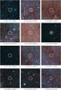 |
Fig. 12
Objects from Table 3 with a rank of 1, thus excellent candidates for a massive star. The color scheme for these images is the same as for Fig. 7. Each image is 10′′ on a side, with the Spitzer point spread function of 1.̋7 shown as a white circle. North is up and East is left. |
| Open with DEXTER | |
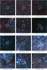 |
Fig. 13
More objects from Table 3 with a rank of 1, thus excellent candidates for a massive star. The color scheme for these images is the same as for Fig. 7. Each image is 10′′ on a side, with the Spitzer point spread function of 1.̋7 shown as a white circle. North is up and East is left. |
| Open with DEXTER | |
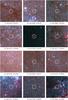 |
Fig. 14
More objects from Table 3 with a rank of 1, thus excellent candidates for a massive star. The color scheme for these images is the same as for Fig. 7. Each image is 10′′ on a side, with the Spitzer point spread function of 1.̋7 shown as a white circle. North is up and East is left. |
| Open with DEXTER | |
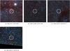 |
Fig. 15
More objects from Table 3 with a rank of 1, thus excellent candidates for a massive star. The color scheme for these images is the same as for Fig. 7. Each image is 10′′ on a side, with the Spitzer point spread function of 1.̋7 shown as a white circle. North is up and East is left. |
| Open with DEXTER | |
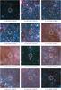 |
Fig. 16
Objects from Table 3 with a rank of 2, thus decent candidates for a massive star. The color scheme for these images is the same as for Fig. 7. Each image is 10′′ on a side, with the Spitzer point spread function of 1.̋7 shown as a white circle. North is up and East is left. |
| Open with DEXTER | |
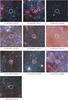 |
Fig. 17
More objects from Table 3 with a rank of 2, thus decent candidates for a massive star. The color scheme for these images is the same as for Fig. 7. Each image is 10′′ on a side, with the Spitzer point spread function of 1.̋7 shown as a white circle. North is up and East is left. |
| Open with DEXTER | |
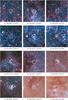 |
Fig. 18
Objects from Table 3 with a rank of 3, thus not good candidates for a massive star. The color scheme for these images is the same as for Fig. 7. Each image is 10′′ on a side, with the Spitzer point spread function of 1.̋7 shown as a white circle. North is up and East is left. |
| Open with DEXTER | |
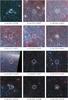 |
Fig. 19
More objects from Table 3 with a rank of 3, thus not good candidates for a massive star. The color scheme for these images is the same as for Fig. 7. Each image is 10′′ on a side, with the Spitzer point spread function of 1.̋7 shown as a white circle. North is up and East is left. |
| Open with DEXTER | |
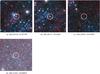 |
Fig. 20
More objects from Table 3 with a rank of 3, thus not good candidates for a massive star. The color scheme for these images is the same as for Fig. 7. Each image is 10′′ on a side, with the Spitzer point spread function of 1.̋7 shown as a white circle. North is up and East is left. |
| Open with DEXTER | |
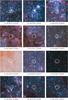 |
Fig. 21
Objects from Table 3 with a rank of 4, thus very poor candidates for a massive star. The color scheme for these images is the same as for Fig. 7. Each image is 10′′ on a side, with the Spitzer point spread function of 1.̋7 shown as a white circle. North is up and East is left. |
| Open with DEXTER | |
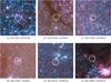 |
Fig. 22
More objects from Table 3 with a rank of 4, thus very poor candidates for a massive star. The color scheme for these images is the same as for Fig. 7. Each image is 10′′ on a side, with the Spitzer point spread function of 1.̋7 shown as a white circle. North is up and East is left. |
| Open with DEXTER | |
 |
Fig. 23
Objects from Table 3 with a rank of 5, thus extremely poor candidates for a massive star. The color scheme for these images is the same as for Fig. 7. Each image is 10′′ on a side, with the Spitzer point spread function of 1.̋7 shown as a white circle. North is up and East is left. |
| Open with DEXTER | |
© ESO, 2015
Current usage metrics show cumulative count of Article Views (full-text article views including HTML views, PDF and ePub downloads, according to the available data) and Abstracts Views on Vision4Press platform.
Data correspond to usage on the plateform after 2015. The current usage metrics is available 48-96 hours after online publication and is updated daily on week days.
Initial download of the metrics may take a while.