| Issue |
A&A
Volume 578, June 2015
|
|
|---|---|---|
| Article Number | A101 | |
| Number of page(s) | 25 | |
| Section | Stellar atmospheres | |
| DOI | https://doi.org/10.1051/0004-6361/201525687 | |
| Published online | 11 June 2015 | |
Online material
Movie of Fig. 6
Appendix A: Doppler images for the seasons 2007/08 to 2011/12
Appendix A.1: Season 2007/08
In Fig. A.1 five almost consecutive Doppler images are shown, which cover around eight rotations. In Fig. A.2 the spot-model fits of the Doppler images are shown.
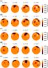 |
Fig. A.1
Doppler images of XX Tri for the observing season 2007/08. Each DI is shown in four spherical projections separated by 90°. The rotational shift between consecutive images is corrected, i.e., the stellar orientation remains the same from map to map and from season to season. The time difference between each Doppler image is indicated in units of rotational phase φ. |
| Open with DEXTER | |
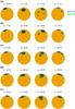 |
Fig. A.2
Spot-model fits of the Doppler images in Fig. A.1. Each spot is shown with different color/contrast for better visualization. |
| Open with DEXTER | |
Appendix A.2: Season 2008/09
In Fig. A.3 seven almost consecutive Doppler images are shown, which cover around nine rotations. In Fig. A.4 the spot-model fits of the Doppler images are shown.
|
Fig. A.3
Doppler images of XX Tri for the observing season 2008/09. Otherwise as in Fig. A.1. |
|
| Open with DEXTER | |
|
Fig. A.4
Spot-model fits of the Doppler images in Fig. A.3. Otherwise as in Fig. A.2. |
|
| Open with DEXTER | |
Appendix A.3: Season 2009/10
In Fig. A.5 five almost consecutive Doppler images are shown, which cover around eight rotations. In Fig. A.6 the spot-model fits of the Doppler images are shown.
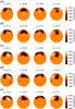 |
Fig. A.5
Doppler images of XX Tri for the observing season 2009/10. Otherwise as in Fig. A.1. |
| Open with DEXTER | |
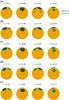 |
Fig. A.6
Spot-model fits of the Doppler images in Fig. A.5. Otherwise as in Fig. A.2. |
| Open with DEXTER | |
Appendix A.4: Season 2010/11
In Fig. A.7 five almost consecutive Doppler images are shown, which cover around nine rotations. In Fig. A.8 the spot-model fits of the Doppler images are shown.
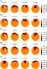 |
Fig. A.7
Doppler images of XX Tri for the observing season 2010/11. Otherwise as in Fig. A.1. |
| Open with DEXTER | |
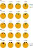 |
Fig. A.8
Spot-model fits of the Doppler images in Fig. A.7. Otherwise as in Fig. A.2. |
| Open with DEXTER | |
Appendix A.5: Season 2011/12
In Fig. A.9 seven almost consecutive Doppler images are shown, which cover around ten rotations. In Fig. A.10 the spot-model fits of the Doppler images are shown.
|
Fig. A.9
Doppler images of XX Tri for the observing season 2011/12. Otherwise as in Fig. A.1. |
|
| Open with DEXTER | |
|
Fig. A.10
Spot-model fits of the Doppler images in Fig. A.9. Otherwise as in Fig. A.2. |
|
| Open with DEXTER | |
Appendix B: Line profiles of Doppler images for the seasons 2006/07 to 2011/12
Figures B.1 and B.2 show the observed and inverted line profiles of each Doppler image for all observational seasons.
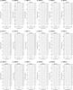 |
Fig. B.1
Line profiles of Doppler images #1–18. Each figure shows the observed (solid lines) and inverted (dotted lines) line profiles for one Doppler image stating their mid times and the respective phases. Rotation advances from bottom to the top. Their corresponding rms-errors are given in Table 3. |
| Open with DEXTER | |
 |
Fig. B.2
Line profiles of Doppler images #19-36. Otherwise as in Fig. B.1. |
| Open with DEXTER | |
Appendix C: Phase coverage of Doppler images for the seasons 2006/07 to 2011/12
Figure C.1 shows the phase coverage of each Doppler image for all observational seasons.
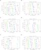 |
Fig. C.1
Phase coverage of Doppler images from 2006 to 2012. Different filled (colored) symbols represents the phases of each individual Doppler image, whereas not-filled circles represents non-used spectra (except for gap filling). The arrows indicate the spectra, which were used to fill up large observational gaps. Detailed information is given in Table 3. |
| Open with DEXTER | |
Appendix D: CCF-maps and DR-fits for the seasons 2006/07 to 2011/12
Figure D.1 shows the ccf maps from each observing season. In Fig. D.2 the observed differential rotation pattern determined from the ccf maps, together with the best fit of the differential rotation following Eqs. (5) and (6) are shown.
|
Fig. D.1
Cross-correlation function maps from 2006 to 2012. Each map represents the average ccf map for one observing season. |
|
| Open with DEXTER | |
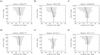 |
Fig. D.2
Differential rotation signatures from 2006 to 2012. Analyzing the ccf maps in Fig. D.1 reveals a weak solar-like differential rotation. The dots are the correlation peaks per 5°-latitude bin and their error bars are defined as the FWHMs of the corresponding Gaussians. The dashed line represents a fit using Eq. (5), whereas the solid line represents a fit using Eq. (6). The parameters for each fit are summarized in Table 5. |
| Open with DEXTER | |
Appendix E: Longitudinal spot distribution for the seasons 2006/07 to 2011/12
Figure E.1 shows the mean distribution of the spot area from our spot-model fits for each observing season.
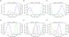 |
Fig. E.1
Longitudinal spot area distribution on XX Tri from 2006 to 2012. Shown are the seasonal mean distributions of the individual spots (solid colored lines) from our spot-model fits for each observing season. The black dashed line represents the total spotted area. The spot area is given in solar hemispheres on the left axis (1 SH=3.05 Gm2) and relative to the total area of a stellar hemisphere of XX Tri on the right axis. |
| Open with DEXTER | |
© ESO, 2015
Current usage metrics show cumulative count of Article Views (full-text article views including HTML views, PDF and ePub downloads, according to the available data) and Abstracts Views on Vision4Press platform.
Data correspond to usage on the plateform after 2015. The current usage metrics is available 48-96 hours after online publication and is updated daily on week days.
Initial download of the metrics may take a while.