| Issue |
A&A
Volume 577, May 2015
|
|
|---|---|---|
| Article Number | L6 | |
| Number of page(s) | 9 | |
| Section | Letters | |
| DOI | https://doi.org/10.1051/0004-6361/201526243 | |
| Published online | 21 May 2015 | |
Online material
Appendix A: Column density map of Orion A
We have generated reduced data products for the Orion A region using HIPE processing to level 1 followed by final level 2 Scanamorphos processing (version 24.0, using the galactic option, Roussel 2013). The column density (and temperature) maps were derived in a similar way as those presented in Stutz et al. (2010, 2013) and Launhardt et al. (2013), with the total power emission levels at each of the four wavelengths calculated using Planck and IRAS data (Bernard et al. 2010). We briefly summarize the steps we used to generate the N(H) and temperature maps here and refer to the above works for more details. We applied the total power emission level corrections for each of the 160 μm, 250 μm, 350 μm, and 500 μm intensity maps (Bernard et al. 2010). We convolved the data to the largest beam: the 500 μm beam, with ~38′′ FWHM. We used the azimuthally averaged convolution kernels from Aniano et al. (2011). We then re-gridded the data to a matched coordinate system and pixel scale, in this case, we adopted an 18′′ pixel scale (see Appendix B for more details). The conversion to matched units assumes the beam sizes listed in the SPIRE instrument handbook. We fit the SED of each pixel assuming a modified blackbody function of the form ![]() (A.1)where Ω is the solid angle of the emitting element, Bν(Td) is the Planck function at a dust temperature Td, and τ(ν) is the optical depth at frequency ν. Here, the optical depth is given by
(A.1)where Ω is the solid angle of the emitting element, Bν(Td) is the Planck function at a dust temperature Td, and τ(ν) is the optical depth at frequency ν. Here, the optical depth is given by ![]() , where NH = 2 × N(H2) + N(H) is the total hydrogen column density, mH in the proton mass, κν is the assumed frequency dependent dust opacity law, and Rgd is the gas-to-dust ratio, assumed to be 110 (Sodroski et al. 1997). We used the Ossenkopf & Henning (1994) model dust opacities corresponding to Col. 5 of their Table 1 (sometimes referred to as the OH5 opacities). These opacities are meant to reflect grains with thin ice mantles after 105 years of coagulation time at an assumed gas density of 106 cm-3. See Stutz et al. (2013) and Launhardt et al. (2013) for discussions on the systematic uncertainties introduced by the model dust opacity assumption. To apply the color and beam size corrections recommended in the SPIRE and PACS instrument handbooks, we first fit the uncorrected pixel SED to estimate the temperature. We then applied the interpolated correction value at that temperature and re-fit the SED.
, where NH = 2 × N(H2) + N(H) is the total hydrogen column density, mH in the proton mass, κν is the assumed frequency dependent dust opacity law, and Rgd is the gas-to-dust ratio, assumed to be 110 (Sodroski et al. 1997). We used the Ossenkopf & Henning (1994) model dust opacities corresponding to Col. 5 of their Table 1 (sometimes referred to as the OH5 opacities). These opacities are meant to reflect grains with thin ice mantles after 105 years of coagulation time at an assumed gas density of 106 cm-3. See Stutz et al. (2013) and Launhardt et al. (2013) for discussions on the systematic uncertainties introduced by the model dust opacity assumption. To apply the color and beam size corrections recommended in the SPIRE and PACS instrument handbooks, we first fit the uncorrected pixel SED to estimate the temperature. We then applied the interpolated correction value at that temperature and re-fit the SED.
In an additional step, we used the 500 μm resolution temperature (Td) map to convert the 250 μm intensity map to a column density map to improve the final resolution (Figs. A.1 and 1). Both maps compare well; only minor differences are apparent on the smallest scales caused by resolution effects, as expected. The previously published Herschel-derived N(H) maps compare well to the maps we present here (e.g., Lombardi et al. 2014; Polychroni et al. 2013).
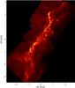 |
Fig. A.1
Orion A N(H) map, shown on a log scale. |
| Open with DEXTER | |
Appendix B: Fitting N(H) PDFs without binning
Here we describe the method we used to fit an index α to a power-law distribution of the form dN/ dZ ∝ Zα over a finite range in Z values from Zmin to Zmax. The differential probability of the column density Zi, given a power-law distribution Zα and total number of expected detections nexp in the interval between Zmin and Zmax , is ![]() The likelihood ℒ is given by the product of the individual probabilities, or
The likelihood ℒ is given by the product of the individual probabilities, or 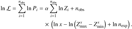 It is straightforward to show that the likelihood is maximized when the models are restricted to those with nexp = nobs. Hence, we simplify the notation by n = nexp = nobs and obtain
 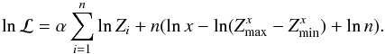 To determine where ℒ is maximized, we differentiate w.r.t. α (or x = α + 1) and set to zero
 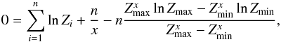 which can be rewritten as
 ![]() where
where  The error is given by Gould (1995) Eq. (2.4):
  which can be written more elegantly as
  This expression can be Taylor-expanded:
  (B.1)Equation (B.1) represents the analytical error solution assuming the power-law model accurately reflects the distribution of data values. Therefore it represents a lower limit for the errors. Alternatively, the errors can be estimated using the Δ χ2 = 1.0 interval, which compares well to those derived using the minimum-variance bound (see Table B.1 for a comparison between the two). The power-law indices and Δ χ2 = 1.0 errors are listed in Table 1.
Comparison of power-law index errors.
Appendix B.1: Effects of resolution, pixel-size, and fitting range on the power-law index
As described above, the power-law indices for each region were extracted from 18′′ pixel N(H) maps derived from the 250 μm map of Orion A. Here we test the effect of adopting different pixel scales for the 250 μm N(H) map. As shown in Fig. B.1, the adopted pixel scale has a negligible effect on the indices, with a strongest effect on the best-fit indices of ~ 2%. The fractional errors increase with pixel size because the number of pixels decreases. We found similar results using the 500 μm N(H) map (with a beam size of ~36′′ FWHM) and adopting pixel sizes of 10′′, 20′′, 30′′, and 40′′: the power-law index is only marginally affected by the choice in pixel size. The fractional errors exhibit the same behavior as for the 250 μm, but are somewhat larger (at most 10% at 40′′) because of the smaller number of pixels available to fit. Finally, in Fig. B.2 we compare the indices derived from the 250 μm 18′′ pixel map with those derive from the 500 μm 40′′ pixel map. The two slope estimates agree well.
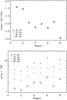 |
Fig. B.1
Top: best-fit power-law index for each region as a function of N(H) map pixel size. The slope values are not affected by correlated pixel, and differences are 2% at most. Bottom: error for each region as a function of N(H) map pixel size. The error increases with pixel size because the number of counts decreases. All quantities shown here have been derived using the same N(H) limits presented in Table 1. |
| Open with DEXTER | |
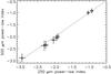 |
Fig. B.2
Indices derived from the 250 μm 18′′pixel map vs. those derived from the 500 μm 40′′pixel map, both using the N(H) limits presented in Table 1. |
| Open with DEXTER | |
We also tested varying the upper bound of the fitting range shown as Max log N(H) in Table 1. For a change ± Δlog N(H) = 0.3, the indices change by ~10% or less; this variation is much smaller than the differences between regions.
Appendix C: Effects of completeness and extinction on the Class 0 protostar fraction
Appendix C.1: Completeness of protostellar catalogs
The northern portion of Orion A (regions 1 and 2) are most affected by incompleteness because of the elevated levels of nebulosity. We estimated the completeness limit in the HOPS protostellar catalog as follows. We injected artificial sources into the 70 μm images and recovered them with our source-finding software (see Stutz et al. 2013, for details). We estimated the mean 90% completeness level for regions 1 and 2 to be 0.12 Jy, while for the rest of L1641 it is 0.03 Jy. We therefore applied a 0.12 Jy 70 μm flux limit to the HOPS protostar catalog, eliminating about 10% of protostars from the catalog. We then calculated Class 0 fractions from the remaining sources. The completeness-corrected and total raw sample fractions agree well, as shown in Fig. C.1.
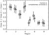 |
Fig. C.1
Class 0 fraction in regions. Diamonds indicate the total fraction (Table 1), while squares indicate the completeness corrected values. Results remain consistent with and without the application of the completeness limit. |
| Open with DEXTER | |
Appendix C.2: Effect of foreground extinction on Tbol
Our goal is to assess the effects of foreground extinction on the Tbol-based YSO classification. We assumed here that the main contribution to an erroneous Tbol classification is the misidentification of Class I sources as Class 0 protostars (Tbol) < 70 K). While other sources of contamination are also possible, scrutiny of the HOPS protostellar SEDs reveals that the current classification based on observed colors and fluxes, in combination with PACS and 870 μm data, is robust (Furlan et al., in prep.).
Upper limits to the distribution of protostellar extinction per region.
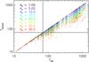 |
Fig. C.2
Model Tbol values versus extincted SED Tbol,ext values. Colors indicate the assumed levels of extinction. Here we show 500 randomly chosen models. As the extinction AV increases, the model Tbol,ext decreases and the levels of contamination at Tbol,ext< 70 K increases. |
| Open with DEXTER | |
We obtained observational constraints on the levels of foreground extinction toward individual protostars from the Herschel N(H) map. We measured the N(H) toward each protostar using an annulus of size 18″ × [1.5,4] (or ~11 400 AU to 30 300 AU), adopted to avoid extinction intrinsic to the protostellar envelopes. Within each annulus we calculated the median value of N(H). In Table C.1 we list the median, minimum, and maximum protostellar N(H) values for each region, assuming a conversion of AV/N(H) = 1.85 × 10²¹ mag cm-2 (e.g., Bohlin et al. 1978,derived for the diffuse ISM, and used here for notational simplicity). These values are upper limits because the N(H) map integrates the extinction through the entire cloud. The protostellar AV values have at most 35 mag in regions 1 and 7. However, more typical values range from ~20 mag to ~10 mag.
To assess the levels of contamination in the Class 0 sample, we used the protostellar model grid presented in Stutz et al. (2013). We refer to this publication and to Furlan et al. (in prep.) for more details. In brief, we varied five parameters in our grid: the inclination of the disk relative to the LOS, the envelope density, the cavity opening angle, the disk size, and the luminosity of the central protostar. Our grid contains uniformly sampled paramaters and uses the Ormel et al. (2011) model dust opacities (icsgra3). In total, our grid contains 30 400 individual models. About ~30% of the models have Tbol< 70 K, similar to the observed protostellar distribution. We attenuated each model SED (adopting the wavelength coverage of the observations) with a range of AV values between 1 and 35 mag, spanning the observed range in AV toward the protostar sample (Table C.1). For consistency with the above protostellar YSO measurements, we attenuated the model SEDs with the same model as that used to derive the N(H) map (Ossenkopf & Henning 1994; OH5), assuming AV/AK = 14 (Nielbock et al. 2012). In Fig. C.2 we show the resulting extincted Tbol,ext values as a function of Tbol for a random subset of models. We then measured the fraction of models that have Tbol> 70 K and Tbol,ext< 70 K as a function of Tbol and AV, marginalizing over a uniform AV distribution. The probability that a given Class I protostar is masquerading as a Class 0 protostar is shown in Fig. C.3, top panel. The bottom panel of Fig. C.3 shows the probability that a given Class 0 protostar is correctly identified (has Tbol< 70 K).
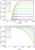 |
Fig. C.3
Top: probability that a source with a given Tbol> 70 K will have Tbol,ext< 70 K, marginalizing over a uniform foreground AV extinction distribution up to the listed value (shown in color). There is no Class 0 contamination from Class I models with Tbol> 400 K for the AV values we consider here. Bottom: probability that a source is correctly classified as a Class 0 source (has Tbol< 70 K). |
| Open with DEXTER | |
We obtained a maximum fraction of ~9% of Class I sources that may appear as Class 0 protostars if models are extincted by up to AV = 35 mag. For all models with Tbol> 400 K, there is zero contamination of Class 0 sources up to extinctions of AV ~ 60 mag. We conclude that the main source of extinction-driven contamination on the Class 0 sample is therefore from Class I sources with 70 K <Tbol< 400 K. We also find that there is < 5% contamination of Class 0 protostars below Tbol,ext~ 45 K and below foreground extinction levels of AV = 35 mag. For a median extinction value of AV = 20 mag, the fraction of Class 0 contamination is lower than 5% for Tbol,ext< 55 K.
Using the total contamination fractions shown in Fig. C.3 and both the median and maximum observed AV levels (Table C.1), we applied correction factors to the observed numbers of Class 0 protostars, keeping the total number of YSOs fixed at the observed value. The dependence of the Class 0 fraction on extinction contamination is presented in Fig. C.4. While the overall amplitude of the fraction is affected by the foreground extinction effects, the shape is not. As noted above, the bottom panel of Fig. C.3 demonstrates that at Tbol,ext< 55 K the amount of Class 0 contamination is lower than 5% for our expected levels of extinction. We therefore tested the effects of adopting a 55 K division between Class 0 and Class I protostars. The results are similar to those shown in Fig. C.4 for the median extinction-corrected values, as expected. We therefore conclude that contamination driven by foreground extinction cannot account for the observed trend presented in Fig. 3.
We note that our requirement of a PACS 70 μm detection and the inclusion of longer wavelengths covering the peak of the cold-dust SED, in combination with meticulous short-wavelength selection (Megeath et al. 2012), virtually guarantees the presence of an envelope. Therefore we do not consider Class I protostar contamination from more evolved sources to be a significant source of error (see also Heiderman & Evans 2015).
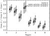 |
Fig. C.4
Dependence of the fraction of Class 0 protostars on Tbol misclassification due to foreground extinction. Diamonds indicate the raw uncorrected observed fractions. Squares indicate the fractions derived by correcting for the sample median AV extinction levels toward protostars in each region. X-symbols indicate the fractions derived by correcting for the maximum AV observed toward protostars in each region. |
| Open with DEXTER | |
© ESO, 2015
Current usage metrics show cumulative count of Article Views (full-text article views including HTML views, PDF and ePub downloads, according to the available data) and Abstracts Views on Vision4Press platform.
Data correspond to usage on the plateform after 2015. The current usage metrics is available 48-96 hours after online publication and is updated daily on week days.
Initial download of the metrics may take a while.