| Issue |
A&A
Volume 573, January 2015
|
|
|---|---|---|
| Article Number | A59 | |
| Number of page(s) | 43 | |
| Section | Extragalactic astronomy | |
| DOI | https://doi.org/10.1051/0004-6361/201423485 | |
| Published online | 18 December 2014 | |
Appendix A: Tables
In this appendix, we summaryze the main photometric parameters of the galaxies in the sample (Table A.1) obtained (within the CALIFA collaboration) from SDSS r-band images of the galaxies in the sample (see Walcher et al., in prep., for details). In Table A.1 columns correspond to:
-
Columns [1] and [2]: object and CALIFA unique ID number for the galaxy, respectively.
-
Columns [3] and [4]: systemic velocity and position angle of the apparent major axis obtained from NED.
-
Columns [5]: effective radius in arcsec of the disk estimated as detailed in Sánchez et al. (2014).
-
Columns [6]: radial distance (in units of the effective radii) used to estimate the large-scale photometric position angles (in column 8) and ellipticities (in Col. 9).
-
Columns [7] and [8]: morphological position angles at one effective radius (PAre) and at the largest scale of the SDSS images (PAout). Both measurements were inferred from the SDSS r-band image of the galaxy using the IRAF task ellipse.
-
Column [9]: ellipticity of the outer isophotes of the SDSS r-band image obtained using the IRAF task ellipse.
-
Column [10]: identification of the galaxy as isolated (I G), interacting/merging (IoM G), or group of galaxies (GoG; see Sect. 2.3 for criteria on this division). Here, we divide the interacting sample analyse in the work (pair of galaxies, small groups of galaxies and mergers with tidal features) in IoM G and GoG just for reference to future works.
-
Column [11]: morphological type from visual classification performed by the CALIFA collaboration (see H13 and Walcher et al., in prep., for details).
-
Column [12]: bar strength of the galaxy as an additional outcome of the CALIFA visual classification (see H13 and Walcher at al., in prep., for details). We divided the galaxies into non-barred (A), weakly barred (AB) and strongly barred (B).
-
Column [13]: nuclear type of the object indicating the main ionization mechanisms in the central region determined through diagnostic diagrams (see Sect. 2.3). SF, LINERS and AGN indicate pure star formation, low-ionization nuclear emission-line regions and AGN, respectively. INDEF indicates that the nuclear type could not be inferred (see Sect. 2.3).
In Table A.2 we include the kinematic parameters directly derived from the measured radial velocities of the Hα+[N ii] emission lines for each galaxy. Each column corresponds to:
-
Column [1]: CALIFA ID number for the galaxy.
-
Column [2]: classification of the galaxy according to the structures in the velocity gradient map obtained from the Hα+[N ii] velocity field. SGP, MGP, and UGP indicate Single, Multi and Unclear velocity Gradient Peak (see Sect. 4.1.2).
-
Columns [3] and [4]: position (in arcsec) of the kinematic center (right ascension [4], and declination [5]) relative to the central spaxel of the CALIFA data cube (see Table 4 in H13 for keyword) (see Sect. 3.2.2).
-
Column [5]: average velocity (in km s-1) in an aperture of 3.7 arcsec in radius centered at the location of the kinematic center. Errors correspond to the standard deviation of the average radial velocities.
-
Columns [6] and [7]: position angle of the major kinematic pseudo-axis estimated from the receding ([6]) and approaching ([7]) sides of the velocity field and taking the reference position at the kinematic center. Errors correspond to the standard deviation of the polar coordinates of the spaxels tracing these axes (see Sect. 3.2.3).
-
Column [8]: position angle of the minor kinematic pseudo-axis. Errors correspond to the standard deviation of the polar coordinates tracing this axis (see Sect. 3.2.3).
-
Column [1]: object.
-
Columns [2]−[5]: sytemic velocities derived from: [2] [O ii] (
 ); [3] [O iii] (
 ); [4] Hα+[N ii] (
 ); and [5] [SII] (
 ) emission lines.
 -
Columns [6]−[8]: class and types of asymmetries detected in the [O iii] profiles (see Sects. 3.3 and 4.2).
Morphological parameters of the sample of CALIFA galaxies analized in this work.
Kinematic parameters estimated directly from the radial velocity derived for each spectra of the CALIFA data cubes with a S/N> 6 (in both the stellar and ionized gas components) through the application of the cross-correlation technique in the Hα+[N ii] spectral range.
Types and classes of asymmetries detected from the [O iii] emission line profiles.
Appendix B: Presence of double/multiple gaseous components: detection limits for CALIFA V500 spectra
The capability of detecting double-peaked/multi-component emission-line profiles in the spectra of galaxies strongly depends on the spectral resolution as well as on its S/N. In this appendix we analize the capabilities and limitations of the CALIFA V500 data for such detection.
Appendix B.1: Noise influence
For an ideal Gaussian profile, the difference in velocity between the peak and the bisector velocity at any intensity level (ΔVb hereafter) is zero, but the presence of noise and the limited spectral resolution of the data would be perturbing this behavior. Figure B.1 shows two examples of a Gaussian model for a single and a double-component emission line profiles for the same spectral resolution than CALIFA V500, including the shape of their bisectors. We note the difference between the actual bisector (blue line in Fig. B.1) and the ideal bisector of a single non-perturbed Gaussian (dotted line in Fig. B.1). In order to determine the limits on the detection of double/multiple gaseous components in the CALIFA V500 spectra, an isolated emission line (e.g., [O iii] λ5007) has been modeled through a single Gaussian profile using the same spectral sampling than the CALIFA V500 configuration. The width of this Gaussian profile was selected to be the instrumental FWHM (6 Å, see H13) and a set of central wavelengths were selected to cover the redshift range of CALIFA (from 1000 to 9000 km s-1 in steps of 500 km s-1). Each of these single-emission line profiles were perturbed by normally-distributed, pseudo-random noise with a mean of zero and a standard deviation of one, obtaining a set of single-Gaussian profiles of S/N ranging from 5 to 110. The S/N was estimated from the ratio of the flux at the peak of the perturbed Gaussian profile and the standard deviation in the continuum. Simulations assume a negligible impact on the line profile of the underlaying stellar continuum subtraction.
The bisectors of each profile (1.5 × 10⁶ in total) were traced at twenty intensity levels (from 5% to 100% of the intensity peak in steps of 5%), providing the shift in velocity at each intensity level respect to an unperturbed Gaussian bisector (ΔVb hereafter, see Fig. B.1). Figure B.2 shows the dependence of the measured ΔVb on S/N for the set of single-Gaussian profiles generated. It is clear that a single Gaussian profile at the resolution of CALIFA V500 data could appear as an asymmetric profile at some degree depending on its S/N and the intensity level at which the bisector velocity is measured. Curves drawn in Fig. B.2 at positive and negative ΔVb delimit the region of ΔVb derived from the different spectra in these single-Gaussian experiments. That is, all the ΔVb at a selected bisector level (for a single-Gaussian emission line) are within the region defined by the curves in Fig. B.2 associated with that bisector level. Therefore, if the bisector of an unknown emission line profile is traced and ΔVb at a particular bisector level is in the region between the curves associated with that bisector level in Fig. B.2, we cannot say anything about the presence or not of double components. However, we are confident that an observed profile is the result of at least two gaseous components if a ΔVb is measured at a particular bisector level beyond the curves associated with that level in Fig. B.2. For example, if we have an emission line profile of S/N ~ 60 and we have measured a ΔVb of 50 km s-1 at the intensity level of 10% of the peak (10% bisector level), we do not know if we actually have a single or a double component profile, but if we measured a ΔVb of 50 km s-1 in the same emission line profile at the intensity level of 75% of the peak (75% bisector level) we are confident that we have a double/multiple components.
|
Fig. B.1
a) Single-Gaussian model (including random noise) of an single emission line (S/N ~ 45) for CALIFA V500. The bisector of a symmetric profile should remain at constant velocity (or wavelength) for all intensity levels, dividing it into two equal parts; any existing asymmetry between the base and the peak of the line will remain reflected in the shape of the bisector. The dotted vertical line corresponds to the bisector of an ideal symmetric Gaussian profile, while the blue line is the actual bisector of the modeled profile, which deviates from the ideal bisector due to noise and velocity sampling. Dashed lines only indicate some intensity levels (in percentage of the intensity peak) that are refered to as “bisector levels”. b), b1) Resultant profile (black line) from the combination of two Gaussian components. Both Gaussians profiles have similar velocity dispersions, a flux ratio of 0.3 and a velocity shift of 300 km s-1 (red and green dashed curves). The blue line is the bisector of the resultant profile and the dotted vertical line is the same as in a). b), b2) Zoom of the profile in b1). Horizontal dashed lines indicate the difference in velocity between the central velocity (traced by the dotted line) and the velocity at different bisector levels (ΔVb). |
|
| Open with DEXTER | |
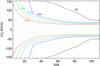 |
Fig. B.2
Noise-induced asymmetries limits, as a function of the S/N, of the difference in velocity between the peak and selected bisector levels (in percentage of the intensity peak, as indicated in the plot) for V500 CALIFA spectra derived from a large number of modeled single-Gaussian profiles. The ΔVb obtained for each selected bisector level are within the curves for that bisector. Any ΔVb beyond these curves should be indicating the presence of secondary gaseous components. |
| Open with DEXTER | |
For S/N between 40 and 90, ΔVb curves can be approched at first order by a linear function of S/N (FΔVb(S/N) hereafter), with the linear coefficients parametrized in terms of bisector levels. Then, for practical applications of searching kinematically distinct gaseous components in V500 CALIFA spectra through unblended emission lines, the FΔVb(S/N) limits at a particular bisector level can be approached through ![]() (B.1)where, l denotes the bisector level, and the polynomial functions of the second degree A(l) and B(l) are
(B.1)where, l denotes the bisector level, and the polynomial functions of the second degree A(l) and B(l) are 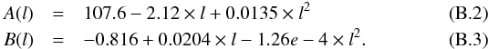 The ΔVb curves in Fig. B.2 are almost constant for S/N ≳ 90, constant value that is approximately the FΔVb(S/N) at S/N = 90 for each bisector level. Then:
 ![]() (B.4)With this simple approach of the ΔVb curves in Fig. B.2, we have a probability smaller than 0.6% of having a ΔVb associated with a single Gaussian profile beyond the limit provided by FΔVb(S/N) at any bisector level and any S/N ≥ 40.
(B.4)With this simple approach of the ΔVb curves in Fig. B.2, we have a probability smaller than 0.6% of having a ΔVb associated with a single Gaussian profile beyond the limit provided by FΔVb(S/N) at any bisector level and any S/N ≥ 40.
Appendix B.2: Parameter space for asymmetries in CALIFA emission line profiles
If we could isolate and observe a single gaseous system in a galaxy, we could derive its parameters (flux, velocity and velocity dispertion) from the ideal Gaussian profiles of its spectrum. The presence of two or more gaseous systems with distinct kinematics along the line of sight would result in complex emission lines in the spectra of the observed object. These profiles can show blueshifted or/and redshifted wings, shoulders and/or double peaks, shapes that are a complex functions of the parameters characterizing each gaseous component.
In this section we explore the parameter space (relative intensity, velocity and velocity dispersion) of two gaseous systems associated with the different profiles classes and types defined in Sect. 4.2. With this aim, we have used a two Gaussians functions to model [O iii] emission line profiles from two gaseous components.We performed a set of experiments playing with the input parameters: (1) the central wavelength of the main component, covering the CALIFA redshift range (from ~1000 to ~9000 km s-1) in steps of 100 km s-1; (2) the FWHM of the main component, changing from 60% to 100% in steps of 10% of the CALIFA V500 instrumental FWHM (6 Å, see H13); (3) the relative intensity ratio of the secondary (Is) and dominant (Id) components, varying from 0.1 to 0.9 in steps of 0.1; (4) the relative difference in velocity (ΔV) between both components, ranging from 0 to 800 km s-1 in steps of 10 km s-1; and (5) the FWHM difference (in Å) of the secondary and dominant components, spaning from 0 to 3 in steps of 0.5. We only generated redshifted asymmetries, assuming that blueshifted profile will follow a similar parameter space but with negative difference in velocity between the main and the secondary components. The resultant profiles were perturbed by normally-distributed, pseudo-random noise with a mean of zero and a standard deviation of one, obtaining S/N values from ~40 to ~100. We classified the simulated profiles showing asymmetries according to the classes and types defined in Sect. 4.2. Asymmetries classes/types result from many combination of the parameters of both Gaussian components. Figure B.3 shows some examples of the possible combinations for relative velocity (| ΔV |) and intensity (Is/Id) providing asymmetric profiles for a range of velocity dispersions for the dominant and secondary components.
|
Fig. B.3
Examples of the parameter space for two Gaussians combined to model asymmetric emission line profiles of the types and classes defined in this work (see Sect. 4.2). Lines encicle the region of possible values of the | ΔV | and Is/Id parameters resulting in an asymmetric profile of the classes a) A0, A1, and A2, b) B0, B1, and B2, and c) C0, C1, and C2 indicated by colors. Each plot includes the velocity dispersion ranges for the secondary (σs ~ [120 − 334] km s-1) and dominant (σs ~ [90 − 154] km s-1) components used to model the profiles. |
|
| Open with DEXTER | |
From the modeled profiles we can also estimate the uncertanties when fitting an asymmetric profile with a single Gaussian model. With this aim, we fit a single Gaussian to all the asymmetric profiles and we compared its flux with the total flux of the two Gaussians forming the modeled profile. For simplicity, noise was not included in these tests. For A0, B0, C0 and C1 profiles, uncertainties in the estimated flux induced using a single Gaussian instead of two Gaussians components are smaller than 0.5% for any combination of the two Gaussians parameters. For A1, B1, and C3 profiles, uncertainties can reach 4%, being smaller than 0.5% in average. Uncertainties larger than 10% in flux can be induced fitting a single Gaussian to B2 and A2 profiles when the absolute difference in velocity between the two components is larger than 300 km s-1. For B2 and A2 profiles coming from two Gaussian with |ΔV|≤ 300 km s-1, flux uncertainties are smaller than 3% when approching the profile by a single Gaussian.
Appendix C: Atlas of ionized gas velocity fields for CALIFA galaxies
In this appendix we present the kinematic maps derived from the CALIFA datacubes for objects in the analyzed sample. In each plot we include narrow band recovered images from the datacubes for [O ii] λλ3726,3728, [O iii] λλ4959,5007, Hα+[N ii] λλ6548,6584, and [SII]λλ6716,6730 emission lines and their velocity fields. We also show the gradient velocity maps obtained from the Hα+[N ii] velocity fields, the pseudo-rotation curves and the location of spectra showing asymmetric profiles, indicative of the presence of kinematically distinct gaseous systems. Panels in each figure correspond to:
- (a)
Narrow band images (stellar continuum subtracted) of (1) [OII]; (2) [OIII]; (3) Hα+[N ii]; and (4) [SII] obtained by integrating the signal in selected spectral bands (see Sect. 3). Maps are normalized to the flux of their brightest spaxel. Contours correspond to the stellar component distribution as traced by a continuum map made from the total flux of the best stellar fit in the spectral range 3800−7000 Åin logarithmic scle (minimum value is −1.65 dex, and step between countours is 0.15 dex).
- (b)
Velocity field obtained by averaging the obtained radial velocities from Monte Carlo simulations. Radial velocities were inferred from cross-correlation in the (1) [OII]; (2) [OIII]; (3) Hα+[N ii]; and (4) [SII] spectral ranges (see Sect. 3).
- (c)
Standard deviation of the radial velocities for each spaxel from Monte Carlo simulations for (1) [OII]; (2) [OIII]; (3) Hα+[N ii]; and (4) [SII] emission lines (see Sect. 3).
- (d)
Sloan Digital Sky Survey r-band image of the object. The hexagonal area drawn is the CALIFA field of view.
- (e)
Velocity gradient map obtained from the Hα+[N ii] velocity field in (b3). Green cross indicate the location of the kinematic center (see Sect. 3.2.2).
- (f)
Distance to the kinematic center (in arcsec) versus the radial velocity for each spectra of the CALIFA data cube with a S/N larger than the threshold. Blue open squares trace the pseudo-rotation curve. Green circles correspond to those spaxels with the lowest difference in velocity to the KC selected to estimate the minor kinematic axis (see Sect. 3.2.3).
- (g)
Location (black squares) of the spectra tracing the pseudo-rotation curve in (f) on the Hα+[N ii] velocity field and tracing the major kinematic pseudo-axis (the same than those marked in blue open squares in (f)). Filled green circles correspond to those spaxels with a similar velocity than the KC (the same than green open circles in (f)) and tracing the minor kinematic axis.
- (h)
Location on the Hα+[N ii] narrow-band image of the spectra showing asymmetric [O iii] λλ4959,5007 profiles. Green, yellow and black squares correpond to profile classes A, B, and C, respectively.
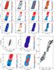 |
Fig. C.1
Summarizing results for IC 2487. |
| Open with DEXTER | |
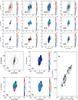 |
Fig. C.2
Summarizing results for IC 0540. |
| Open with DEXTER | |
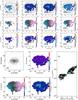 |
Fig. C.3
Summarizing results for IC 0776. |
| Open with DEXTER | |
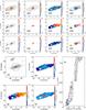 |
Fig. C.4
Summarizing results for IC 0944. |
| Open with DEXTER | |
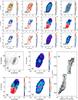 |
Fig. C.5
Summarizing results for IC 1199. |
| Open with DEXTER | |
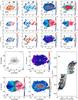 |
Fig. C.6
Summarizing results for IC 1256. |
| Open with DEXTER | |
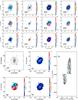 |
Fig. C.7
Summarizing results for IC 1683. |
| Open with DEXTER | |
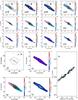 |
Fig. C.8
Summarizing results for IC 2095. |
| Open with DEXTER | |
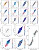 |
Fig. C.9
Summarizing results for IC 2247. |
| Open with DEXTER | |
 |
Fig. C.10
Summarizing results for IC2 487. |
| Open with DEXTER | |
© ESO, 2014
Current usage metrics show cumulative count of Article Views (full-text article views including HTML views, PDF and ePub downloads, according to the available data) and Abstracts Views on Vision4Press platform.
Data correspond to usage on the plateform after 2015. The current usage metrics is available 48-96 hours after online publication and is updated daily on week days.
Initial download of the metrics may take a while.