| Issue |
A&A
Volume 570, October 2014
|
|
|---|---|---|
| Article Number | A2 | |
| Number of page(s) | 20 | |
| Section | Galactic structure, stellar clusters and populations | |
| DOI | https://doi.org/10.1051/0004-6361/201423777 | |
| Published online | 06 October 2014 | |
Online material
Appendix A: Persistence removal
Persistence is a known problem of infrared detectors when observing bright sources. If the exposure time is too long and the source is overexposed, there can be ghost images of the source in a subsequently taken exposure of a faint source. The magnitude of the persistence effect decreases in time according to a power-law (Dressel 2012). To avoid persistence, one should either choose short exposure times or, alternatively, make a sequence of read-outs afterwards, to flush the detector’s memory of the bright source. We took acquisition images right before the object spectra, which lead to persistence in the 2D spectra. Also our 2D sky spectra are affected as we took three dithered images on source before the sky offsets to verify the position on the sky after the drift, and two dithered images on sky that also contain a few stars.
However, we developed a way to remove the persistence signature completely in our sky
frames and to some extent also in the object spectra. We use the images that cause the
persistence and the corresponding 2D spectra that are affected by the persistence.
Removing persistence from the 2D sky spectra is rather straight forward: For every 2D
sky spectrum Sraw,sky we compute
the median of each column along the dispersion axis and subtract it from each pixel in
the column, and do the same with the median along the spatial axis to get a 2D sky
spectrum without any lines or stars Smed,sky. The only
features left in the median subtracted 2D sky spectrum are from the persistence. Then
one can simply compute a corrected 2D sky spectrum Scor,sky (A.1)The clean 2D sky
spectra are combined to 2D Mastersky spectra using IRAF. We also produce noise files for
each sky file that contain the information about the persistence correction.
(A.1)The clean 2D sky
spectra are combined to 2D Mastersky spectra using IRAF. We also produce noise files for
each sky file that contain the information about the persistence correction.
This simple approach is not possible for the 2D object spectra, as there are many stars with strong absorption lines and also an H2 gas emission line. In contrast to the 2D sky spectra, subtracting a median leaves other strong features apart from the persistence residuals. Therefore we decided to model the persistence and subtract the model from the 2D object spectra. To determine the persistence model parameters we use the 2D sky spectra before we apply the aforementioned correction on them.
Saturated pixels have negative counts in our images and leave persistence features in
the 2D spectra taken afterwards. Persistence is also a problem if the counts of a bright
source at a given pixel of the detector are above a certain threshold. First, one needs
to determine the value of this threshold. Therefore we consider only counts above a
trial threshold and make a persistence mask M, where pixel with negative counts in the image
as well as counts above the threshold are set to one and all other pixels are set to
zero. As the raw 2D sky frames are affected by persistence coming from three images on
source and two images on sky, taken ∼2−3 min
later, we make two masks, one for the images on source (Msource) and
one for the sky images (Msky). Then we use
mpfit2dfun.pro (Markwardt
2009) to fit the amplitudes of the persistence, Ksource and
Ksky, and a full-width-half-maximum FWHM
for a Gaussian smoothing filter GFWHM of the masks. The residual
spectrum R
is  (A.2)where the symbol
“∗” denotes convolution.
We try different values of the mask threshold, and we find a minimum of the standard
deviation of the residual spectrum R at a threshold of 33 500 counts. Therefore we
define 33 500 counts as our threshold for further corrections of images taken with an
exposure time of 20 s. For the images with exposure time t = 5 s, we have a lower
threshold of 24 000 counts, found by the same method.
(A.2)where the symbol
“∗” denotes convolution.
We try different values of the mask threshold, and we find a minimum of the standard
deviation of the residual spectrum R at a threshold of 33 500 counts. Therefore we
define 33 500 counts as our threshold for further corrections of images taken with an
exposure time of 20 s. For the images with exposure time t = 5 s, we have a lower
threshold of 24 000 counts, found by the same method.
The next step is to fit Ksource, Ksky, and FWHM
with the chosen threshold value of the mask for every median subtracted 2D sky spectrum
Smed,sky. The
persistence signal decreases in time, therefore Ksource and
Ksky decrease from the first to the
fifth 2D sky spectrum in a sequence. We fit the decrease of K with the power law
 (A.3)where the
parameter A
is the amplitude and γ is a scale factor. We do this for Ksource and
Ksky seperately and together, but our
later analysis shows that we obtain better results when we use the result of fitting
Ksource(t) alone. The
parameters we use are A =
(6900 ± 1700) and γ = (0.98 ± 0.04). The uncertainties are the
formal 1-σ
errors of the fit. With this knowledge we can subtract the persistence from the 2D
object spectra with the equation
(A.3)where the
parameter A
is the amplitude and γ is a scale factor. We do this for Ksource and
Ksky seperately and together, but our
later analysis shows that we obtain better results when we use the result of fitting
Ksource(t) alone. The
parameters we use are A =
(6900 ± 1700) and γ = (0.98 ± 0.04). The uncertainties are the
formal 1-σ
errors of the fit. With this knowledge we can subtract the persistence from the 2D
object spectra with the equation
 (A.4)The images
causing persistence in the 2D object spectra are acquisition images. As we made
acquisition offsets, we subtract persistence caused by the acquisition image itself and
from a shifted acquisition image. We have only the acquisition image itself as file, but
we can identify the shift in pixels from the persistence in the 2D spectra, and we can
fit the shift of the acquisition offset together with an attenuation factor
α. This
factor α is
necessary as the offset was performed before the acquisition image was taken, and
therefore the persistence signal is weaker. In this case the corrected 2D object spectra
Scor,object are
(A.4)The images
causing persistence in the 2D object spectra are acquisition images. As we made
acquisition offsets, we subtract persistence caused by the acquisition image itself and
from a shifted acquisition image. We have only the acquisition image itself as file, but
we can identify the shift in pixels from the persistence in the 2D spectra, and we can
fit the shift of the acquisition offset together with an attenuation factor
α. This
factor α is
necessary as the offset was performed before the acquisition image was taken, and
therefore the persistence signal is weaker. In this case the corrected 2D object spectra
Scor,object are
 (A.5)With these
procedures it is possible to remove the persistence structures completely from the 2D
sky frames and to subtract them from the 2D object spectra partially, but some residuals
still remain. In some cases we made more than one acquisition offset, and furthermore it
is difficult to model the shape of the persistence, which was slightly elliptical due to
the drift during the acquisition. The shape also changes depending on the area on the
detector and seeing conditions. To account for uncertainties in the persistence
subtraction, we make noise files that are used for the further analysis of the spectra.
(A.5)With these
procedures it is possible to remove the persistence structures completely from the 2D
sky frames and to subtract them from the 2D object spectra partially, but some residuals
still remain. In some cases we made more than one acquisition offset, and furthermore it
is difficult to model the shape of the persistence, which was slightly elliptical due to
the drift during the acquisition. The shape also changes depending on the area on the
detector and seeing conditions. To account for uncertainties in the persistence
subtraction, we make noise files that are used for the further analysis of the spectra.
To check the influence of the persistence after the correction on our results we compare two 2D spectra that cover almost the same region of the Milky Way nuclear star cluster. One 2D spectrum was not affected by the persistence, since it was the 20th exposures taken after the acquisition image. The other 2D spectrum was taken shortly after the acquisition image and was affected by persistence. We extract several 1D spectra by summing between 45 and 100 rows of the 2D spectra. Then we fit the CO absorption lines with ppxf. The S/N of the spectra taken from the file with persistence, but after our correction, is lower by ∼27% compared to the S/N of spectra from the file with no persistence. But as the effect of persistence decreases in time, not all of our data are as much affected. We estimate that in ∼70% of our spectra the decrease in S/N due to the persistence is less than 20%.
Appendix B: H2 gas emission Kinematics
We fitted the 1−0 Q(1) 2.4066 μm transition of H2 to make a comparison with previous studies (e.g. Gatley et al. 1986; Yusef-Zadeh et al. 2001; Lee et al. 2008). The excellent agreement of our flux and kinematic maps with these studies shows that our data can reproduce previous results without strong biases. Figure B.1 illustrates the results of the fitting for flux, velocity and velocity dispersion. Regions where the flux was too low and confusion with sky line residuals might be possible are not displayed. In the H2 velocity map we can identify the northeastern and southwestern lobe of the circumnuclear disk (see Fig. 1 of Amo-Baladrón et al. (2011) for an illustration of the central 12 parsec).
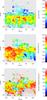 |
Fig. B.1
Results of the single Gaussian fit to the H2 gas emission line. Upper panel: flux in logarithmic scaling and with respect to the maximum flux. Middle panel: velocity in km s-1. Lower panel: velocity dispersion in km s-1, corrected for the instrumental dispersion (σinstr ≈ 27 km s-1). The coordinates are centred on Sgr A* and along the Galactic plane with a position angle of 31.̊40. The cross marks the position of Sgr A*. |
| Open with DEXTER | |
© ESO, 2014
Current usage metrics show cumulative count of Article Views (full-text article views including HTML views, PDF and ePub downloads, according to the available data) and Abstracts Views on Vision4Press platform.
Data correspond to usage on the plateform after 2015. The current usage metrics is available 48-96 hours after online publication and is updated daily on week days.
Initial download of the metrics may take a while.