Online material

Appendix A: Preliminary best-fit solutions

The parameter sets listed in Table A.1 represent the preliminary, coarse model fits to our four observing epochs of LkCa 15 obtained through an iterative search during the early phase of this work. They are used as a starting point for the studies presented in Sects. 5.2 and 5.5. Our final, optimized solutions and their confidence intervals are described in Sect. 5.3.

Appendix B: Best-fit solutions under the restriction of y = 0

Our analysis clearly favors a significant offset y of the disk center that is perpendicular to the line of nodes (cf. Sect. 5.9). However, this offset is yet unconfirmed, and could therefore represent an unknown bias in our modeling approach. For this reason, we here provide an overview of how the imposed restriction of y = 0 would affect our results.

Since some covariances are found between the parameters r, i, g, w and y (cf. Sect. 5.10), the χ² plots for those parameters undergo significant changes. Figures B.1–B.4 show the corresponding plots for the y = 0 parameter sub-space.

In the unrestricted analysis, a range of y values are included in the well fitting family, each of which contributes a narrow valley to the χ² landscape. For parameters that covary with y, the χ² valleys change their positions with varying y; thus, the final χ² valley calculated over all y is broadened. For this reason, imposing the restriction of y = 0 results in steeper χ² curves than in the unrestricted case.

Furthermore, since the natural best-fit value of y is negative, the restriction of y = 0 causes a negative [positive] shift in the best-fit value of parameters that exhibit positive [negative] covariation with y. The gap radius r decreases from 56 AU to 50 AU, whereas the inclination i rises from 50° to 54°.

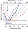Fig. B.1 Constraints on the outer disk wall radius r under the restriction of y = 0. The plot shows the excess of the best-fit χ2 for a given r with respect to the global minimum , which is normalized by the threshold value Δχ2. The color-coded curves represent each individual epoch, whereas the thick black curve is obtained by combining all four epochs. The vertical dotted line marks the best-fit value of r from the unrestricted analysis. The bottom panel shows the well fitting range and the best-fit value for all five analyses.

Open with DEXTER

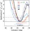Fig. B.2 Constraints on the inclination i of the disk plane under the restriction of y = 0. The plot shows the excess of the best-fit χ2 for a given i with respect to the global minimum , which is normalized by the threshold value Δχ2. The color-coded curves represent each individual epoch, whereas the thick black curve is obtained by combining all four epochs. The vertical dotted line marks the best-fit value of i from the unrestricted analysis. The bottom panel shows the well fitting range and the best-fit value for all five analyses.

Open with DEXTER

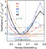Fig. B.3 Constraints on the Henyey-Greenstein parameter g under the restriction of y = 0. The plot shows the excess of the best-fit χ2 for a given g with respect to the global minimum , which is normalized by the threshold value Δχ2. The color-coded curves represent each individual epoch, whereas the thick black curve is obtained by combining all four epochs. The vertical dotted line marks the best-fit value of g from the unrestricted analysis. The bottom panel shows the well fitting range and the best-fit value for all five analyses.

Open with DEXTER

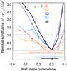Fig. B.4 Constraints on wall shape parameter w under the restriction of y = 0. The plot shows the excess of the best-fit χ2 for a given w with respect to the global minimum , which is normalized by the threshold value Δχ2. The color-coded curves represent each individual epoch, whereas the thick black curve is obtained by combining all four epochs. The vertical dotted line marks the best-fit value of w from the unrestricted analysis, which coincides with the values obtained under y = 0. The bottom panel shows the well fitting range and the best-fit value for all five analyses.

Open with DEXTER

Appendix C: Exploration of disk wall scale height h as an additional free parameter

We ran a small-scale version of the brute-force parameter grid with outer disk scale heights of h = [1,2] to test whether the observed y offset could be an aliasing effect of an inaccurate assumption on h. Since h = 1 represents the hydrostatic equilibrium value, the test value of h = 2 is an extreme case that is intended to probe the possible codependence of h and y with high sensitivity.

The analysis was run only for the best epoch, K3. We used the following parametric grid listed in Table C.1. Its irregularity occurs because it was assembled in two stages after it was found that the first stage did not fully encompass the best-fit solution.

The best-fit solution was achieved for g = 0.70, s = 0, w = 0.05, i = 44°, f = 1.067, and y = −90 mas. The minimum χ² achieved was 601, which is 2.8 Δχ² above the of the best-fit solution with h = 1. While some of the best-fit parameters for h = 2 deviate significantly from their h = 1 counterparts (most notably the wall shape parameter w), we note that the best-fit value for y is still in excellent agreement with the results for h = 1 (y = −70 [ − 115, − 45] mas). This implies that there is no significant covariance between y and h.

This behavior can be understood in conjunction with the observation that the best-fit models do not include a shadow from the inner disk on the wall of the outer disk (s = 0), and thus, the wall appears as a single bright crescent rather than two distinct thin arcs. Increasing the outer disk scale height h makes the crescent wider (thus, perhaps, explaining the reduction in the wall shape parameter w, which is responsible for widening the crescent in the global best fit with h = 1) but does not affect its overall position.

Thus, we conclude that the observed offset in y is a robust result of our analysis within the framework of our disk model and does not reflect an underlying error in the outer disk scale height h. We continue to use h = 1 as a fixed internal parameter for this work.

© ESO, 2014