| Issue |
A&A
Volume 564, April 2014
|
|
|---|---|---|
| Article Number | A63 | |
| Number of page(s) | 16 | |
| Section | Interstellar and circumstellar matter | |
| DOI | https://doi.org/10.1051/0004-6361/201423439 | |
| Published online | 04 April 2014 | |
Online material
Appendix A: The new extinction laws
Based on the issues discussed in Maíz Apellániz (2013a) and the results of experiments 1 and 2, we decided to attempt the calculation of a new family of extinction laws. Ideally, to complete such a task one would use high-quality spectrophotometry from the NIR to the UV of a diverse collection of sources in different environments and with different degrees of extinction. Since such dataset is not available, in this paper we concentrate on only some of the problems discussed in Maíz Apellániz (2013a). More specifically, we will ignore extinction in the UV (except for the region closest to the optical) and for the NIR we will simply use the CCM laws (which, in turn, used Rieke & Lebofsky 1985)12. In other words, we will concentrate on the optical region since that is the critical component for the determination of Teff for OB stars. Ignoring the UV will not matter to a non-specialist interested only in eliminating the extinction from his/her optical data. Ignoring the NIR may matter if the exponent there is significantly different from the CCM one but only if extinction is very large and even then it may only apply to the total extinction correction, not to the determination of Teff from the photometry.
The immediate goals of the new family of extinction laws are:
-
1.
to maintain the overall properties of the CCM laws that havemade them so successful: a single-parameter, easy-to-calculatefamily that covers a large wavelength range; and their overallshape as a function of wavelength (including the functional formin Eq. (C.1));
-
2.
to eliminate the F336W (U-band like) excesses detected in experiment 1, which lead to the temperature biases in experiment 2;
-
3.
to at least alleviate the wiggles induced by the seventh-degree polynomial used by CCM in the optical range and make the new family more similar to the shape derived by Whitford (1958) with spectrophotometry (two straight lines with a knee at x = 2.2μm-1).
To achieve those goals, we use the following strategy:
-
1.
Instead of a seventh-degree polynomial, we [a] select a series ofpoints in x in the optical range, [b] use the values of the CCM laws at these points (with corrections in some cases), and [c] apply a spline interpolation between these points. Note that a spline interpolation was already used by Fitzpatrick (1999).
-
2.
We expand the optical range from x = 1.1–3.3 μm-1 to 1.0–4.2 μm-1 in order to avoid discontinuities and/or knees near the edges of the ranges13.
-
3.
The first two points selected are x = 1.81984 μm-1 and x = 2.27015 μm-1, which correspond to 5495 Å and 4405 Å. The choice is determined by the need to maintain the values of R5495 for a given extinction law. At these values no correction is applied to the CCM laws.
-
4.
A third point is added between x = 1.81984 μm-1 and x = 1.0 μm-1 to minimize the wiggles visible for low and intermediate values of R5495 in CCM and thus make the extinction laws more similar to that of Whitford (1958). After trying different choices, we select x = 1.15μm-1 as the one that produces the smoothest results. Note that the values of the extinction law at exactly these three points are the CCM ones: the changes affect the points in between due to the use of a spline interpolation instead of a seventh-degree polynomial.
-
5.
A fourth point is added between 5495 Å and 4405 Å to maintain the Whitford (1958) knee at its original location near x = 2.2 μm-1 (as it can be seen in Fig. 11, CCM moved the knee towards higher values, i.e. shorter wavelengths, in most cases while the new laws put it back between 2.15 μm-1 and 2.25 μm-1 for most values of R5495). By trial and error we selected x = 2.1 μm-1 and applied a correction to the A(λ)/A(5495) CCM values there of −0.011 + 0.091R5495.
-
6.
Five final points are added between x = 2.27015 μm-1 and x = 4.2 μm-1. Different combinations were tried with the general goals of [a] keeping smooth profiles, [b] correcting the overall F336W excesses found in experiment 1 as a function of E(4405 − 5495), and [c] doing the same as a function of R5495. The final result leads to the points being located at x = 2.7 μm-1, 3.5 μm-1, 3.9 μm-1, 4.0 μm-1, and 4.1 μm-1. The corrections to A(λ)/A(5495) in these points are 0, 0.442 − 1.256/R5495, 0.341 − 1.021/R5495, 0.130 − 0.416/R5495, and 0.020 − 0.064/R5495, respectively. Note that the optical region in CCM ends at x = 3.3 μm-1: for higher values of x the correction is applied to the CCM UV functional form.
Four examples of the new extinction laws are shown in Figs. 11 and 12. An IDL function to obtain the new extinction laws is provided in Table A.1. The validity of the new extinction laws is tested in experiments 3 and 4, i.e. the ones used to iteratively determine them.
IDL coding of the extinction laws in this paper.
Appendix B: CHORIZOS and SED models
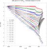 |
Fig. B.1
The Teff–luminosity class distance-calibrated SED family for the LMC developed for CHORIZOS. The black lines are the Geneva/Padova evolutionary tracks between 0.15 M⊙ and 120 M⊙ (a label at the beginning of the track shows the initial mass). Different symbols are used for the luminosity types 0.0, 0.5...5.5. Note that luminosity types are defined at 0.1 intervals but only those at 0.5 intervals are shown for clarity. |
| Open with DEXTER | |
The CHORIZOS code was presented in Maíz Apellániz (2004) as a χ2 Code for Parameterized Modeling and Characterization of Photometry and Spectrophotometry. In subsequent versions, it evolved to become a complete Bayesian code that matches photometry and spectrophotometry to spectral energy distribution (SED) models in up to six dimensions. Some examples of its applications can be seen in Maíz Apellániz et al. (2004a, 2007); Negueruela et al. (2006); Úbeda et al. (2007). The last public version of CHORIZOS, v. 2.1.4, was released in July 2007. Since then, the first author of this paper has been working on versions 3.x, which, among many changes, allow for the use of magnitudes (instead of colors) as fitting quantities and the use of distance as an additional parameter. Problems with the code speed and memory usage did not allow these versions of CHORIZOS to become public (even though the code itself worked for restricted cases). The largest problems have now been solved and a public application with the 3.x version of the code will be publicly available soon.
The use of magnitudes and distances described above leads to the possibility of a new type of stellar SED grids: instead of using Teff and log g as the two parameters, one can substitute log g by luminosity or an equivalent parameter (Maíz Apellániz 2013b). As an intermediate step, one needs to use evolutionary tracks or isochrones that assign the correct value of log g to a given luminosity. We have developed a class of such grids with the following characteristics:
-
1.
There are three separate grids corresponding to the Milky Way,LMC (the ones used in this paper), and SMC metallicities.
-
2.
The luminosity-type parameter is called (photometric) luminosity class and is analogous to the spectroscopic equivalent. To maintain the equivalence as close as possible, its value ranges from 0.0 (hypergiants) to 5.5 (ZAMS).
-
3.
The grids use Geneva evolutionary tracks for high-mass stars and Padova ones for intermediate- and low-mass stars. For the objects in this paper, the relevant tracks are those of Schaller et al. (1992); Schaerer et al. (1993). Note that the use of tracks with rotation would not introduce significant changes in the results of this paper because the purpose of the tracks for O stars are to [a] establish the total range in luminosities and [b] determine the gravity for a given temperature and luminosity. The range in luminosities changes little with the introduction of rotation and the possible changes in gravity at a given grid point can be of the order of 0.2 dex, which leads to an insignificant effect in the optical colors of O stars14.
-
4.
Different SEDs are used as a function of temperature and gravity (or luminosity). For the objects in this paper, the relevant SEDs are the two TLUSTY grids of Lanz & Hubeny (2003, 2007).
-
5.
It is possible to specify a total of five parameters in a given grid: Teff, luminosity class, E(4405 − 5495), R5495, and distance. Note, however, that for most practical applications it is only possible to leave four of these parameters free.
-
6.
For the experiments in this paper we have calculated independent grids with the CCM, F99, and new extinction laws.
Figure B.1 shows the LMC grid used in this paper.
Appendix C: Extinction along a sightline with more than one type of dust
In this paper we make no attempt to disentangle the contributions to the extinction in 30 Doradus among its three possible components: Milky Way (MW), Large Magellanic Cloud (LMC), and internal (30 Dor). The reason for not attempting to do so is the impossibility of doing it with the available data (each component can contribute while being spatially variable, see van Loon et al. 2013). However, that does not affect the validity of our results due to a feature of the extinction law families of CCM and this paper. The extinction laws are written as:  (C.1)where a(λ) and b(λ) are defined by different functional forms in different wavelength ranges (see e.g. Table A.1). A SED with an original form of I0(λ) is extinguished to I(λ) according to:
 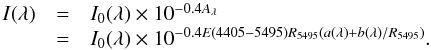 (C.2)Now, suppose that along the sightline to a star there are N clouds, each one of them with a color excess E(4405 − 5495)i and type of extinction R5495,i. The total extinction will be:
 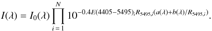 (C.3)It is easy to show that Eqs. (C.2) and (C.3) are equivalent if one defines:
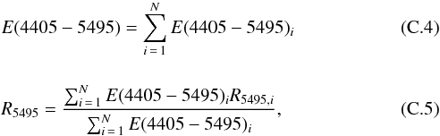 i.e. if each individual extinction law belongs to the same family, then it will represent the combined effect of the N clouds. The total color excess is simply the sum of the individual ones and the type of extinction is the sum of the individual types (characterized by their R5495 values) weighted by the individual color excesses.
© ESO, 2014
Current usage metrics show cumulative count of Article Views (full-text article views including HTML views, PDF and ePub downloads, according to the available data) and Abstracts Views on Vision4Press platform.
Data correspond to usage on the plateform after 2015. The current usage metrics is available 48-96 hours after online publication and is updated daily on week days.
Initial download of the metrics may take a while.