| Issue |
A&A
Volume 562, February 2014
|
|
|---|---|---|
| Article Number | A17 | |
| Number of page(s) | 35 | |
| Section | Stellar structure and evolution | |
| DOI | https://doi.org/10.1051/0004-6361/201321850 | |
| Published online | 03 February 2014 | |
Online material
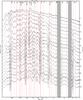 |
Fig. 2
Optical and NIR (interpolated) spectral evolution for SN 2011dh for days 5−100 with a 5 day sampling. Telluric absorption bands are marked with a ⊕ symbol in the optical and shown as grey regions in the NIR. |
| Open with DEXTER | |
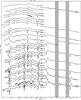 |
Fig. 3
Sequence of the observed spectra for SN 2011dh. Spectra obtained on the same night using the same telescope and instrument have been combined and each spectra have been labelled with the phase of the SN. Telluric absorption bands are marked with a ⊕ symbol in the optical and shown as grey regions in the NIR. |
| Open with DEXTER | |
Optical colour-corrected JC U and S-corrected JC BVRI magnitudes for SN 2011dh.
Optical S-corrected Swift JC UBV magnitudes for SN 2011dh.
Optical colour-corrected SDSS u and S-corrected SDSS griz magnitudes for SN 2011dh.
NIR S-corrected 2MASS JHK magnitudes for SN 2011dh.
MIR Spitzer 3.6 μm and 4.5 μm magnitudes for SN 2011dh.
UV Swift UVW1, UVM2 and UVW2 magnitudes for SN 2011dh.
List of optical and NIR spectroscopic observations.
Pseudo-bolometric UV to MIR lightcurve for SN 2011dh calculated from spectroscopic and photometric data.
Appendix A: Photometric calibration
The optical photometry was tied to the Johnson-Cousins (JC) and Sloan Digital Sky Survey (SDSS) systems. The NIR photometry was tied to the 2 Micron All Sky Survey (2MASS) system. Table A.1 lists the filters used at each instrument and the mapping of these to the standard systems. Note that we have used JC-like UBVRI filters and SDSS-like gz filters at NOT whereas we have used JC-like BV filters and SDSS-like ugriz filters at LT and FTN. The JC-like URI and SDSS-like uri photometry were then tied to both the JC and SDSS systems to produce full sets of JC and SDSS photometry. The Swift photometry was tied to the natural (photon count based) Vega system although the Swift UBV photometry was also tied to the JC system for comparison. The Spitzer photometry was tied to the natural (energy flux based) Vega system.
Mapping of natural systems to standard systems.
Appendix A.1: Calibration method
The SN photometry was calibrated using reference stars within the SN field. These reference stars, in turn, were calibrated using standard fields. The calibration was performed using the SNE pipeline. To calibrate the SN photometry we fitted transformation equations of the type 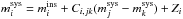 , where
  ,
,  and Zi are the system and instrumental magnitudes and the zeropoint for band i respectively and Ci,jk is the colour-term coefficient for band i using the colour jk. The magnitudes of the SN was evaluated both using these transformation equations and by the use of S-corrections. In the latter case the linear colour-terms are replaced by the S-corrections as determined from the SN spectra and the filter response functions of the natural systems of the instruments and the standard systems. We will discuss S-corrections in Appendix A.5 and compare the results from the two methods. In the end we have decided to use the S-corrected photometry for all bands except the JC U and SDSS u bands. To calibrate the reference star photometry we fitted transformation equations of the type
  , where Xi and ei are the airmass and the extinction coefficient for band i respectively. The magnitudes of the reference stars were evaluated using these transformation equations and averaged using a magnitude error limit (0.05 mag) and mild (3σ) rejection. Both measurement errors and calibration errors in the fitted quantities were propagated using standard methods. The errors in the reference star magnitudes were calculated as the standard deviation of all measurements corrected for the degrees of freedom.
The coefficients of the linear colour terms (Ci,jk) used to transform from the natural system of the instruments to the JC and SDSS standard systems were determined separately. For each instrument, system and band we determined the coefficient by least-square fitting of a common value to a large number of observations. For the NOT and the LT we also fitted the coefficients of a cross-term between colour and airmass for U and B to correct for the change in the filter response functions due to the variation of the extinction with airmass. However, given the colour and airmass range spanned by our observations, the correction turned out to be at the few-percent level and we decided to drop it. Because of the lower precision in the 2MASS catalogue as compared to the Landolt and SDSS catalogues we could not achieve the desired precision in measured 2MASS colour-term coefficients. Therefore we have used synthetic colour-term coefficients computed for a blackbody SED using the NIR filter response functions described in Sect. A.5. The measured JC and SDSS and synthetic 2MASS colour-term coefficients determined for each instrument are listed in Tables A.2–A.4.
JC UBVRI colour-term coefficients for all telescope/instrument combinations.
SDSS ugriz colour-term coefficients for all telescope/instrument combinations.
Appendix A.2: JC calibration
The optical photometry was tied to the JC system using the reference stars presented in Pastorello et al. (2009, hereafter P09 as well as a number of additional fainter stars close to the SN. In the following the reference stars from P09 will be abbreviated as P09-N and those added in this paper as E13-N. Those reference stars, in turn, have been tied to the JC system using standard fields from Landolt (1983, 1992). Taking advantage of the large number of standard star observations obtained with the LT we have re-measured the magnitudes of the P09 reference stars within the LT field of view (FOV). The mean and root mean square (RMS) of the difference was at the few-percent level for the B, V, R and I bands and at the 10-percent level for the U band except for P09-3 which differed considerably. We have also re-measured the magnitudes of the Landolt standard stars and the mean and RMS of the difference was at the few-percent level in all bands. This shows that, in spite of the SDSS-like nature of the LT u, r and i filters, the natural LT photometry transform to the JC system with good precision. In the end we chose to keep the P09 magnitudes, except for P09-3, and use the LT observations as confirmation. The magnitudes of the additional reference stars and P09-3 were determined using the remaining P09 reference stars and large number of deep, high quality NOT images of the SN field. The coordinates and magnitudes of the JC reference stars are listed Table A.5 and their positions marked in Fig. A.1.
 |
Fig. A.1
Reference stars used for calibration of the optical photometry marked on a SDSS r band image. |
| Open with DEXTER | |
Synthetic 2MASS JHK colour-term coefficients for all telescope/instrument combinations.
JC UBVRI magnitudes of local reference stars used to calibrate the photometry.
SDSS ugriz magnitudes for the standard fields PG 0231+051, PG 1047+003, PG 1525-071, PG 2331+046 and Mark-A.
SDSS ugriz magnitudes of local reference stars used to calibrate the photometry.
Appendix A.3: SDSS calibration
The optical photometry was tied to the SDSS system using the subset of the reference stars within the LT FOV. Those reference stars, in turn, have been tied to the SDSS system using fields covered by the SDSS DR8 catalogue (Aihara et al. 2011). The calibration was not straightforward as the SN field and a number of the LT standard fields were not well covered by the catalogue and many of the brighter stars in the fields covered by the catalogue were marked as saturated in the g, r and i bands. The procedure used to calibrate the reference star magnitudes was as follows. First we re-measured the g, r and i magnitudes for all stars marked as saturated using the remaining stars in the LT standard fields covered by the catalogue. We then measured the magnitudes for the stars in the fields not covered by the catalogue and finally we measured the reference star magnitudes using all the LT standard field observations. For reference, our measured SDSS magnitudes for the LT standard fields are listed in Table A.6. Magnitudes of stars covered by the catalogue and not marked as saturated were adopted from the catalogue. The coordinates and the magnitudes of the SDSS reference stars are listed in Table A.7 and their positions marked in Fig. A.1. The magnitudes of P09-3, E13-1 and E13-5 were adopted from the catalogue. The mean and RMS of the difference between measured and catalogue magnitudes for stars with measured and catalogue errors less than 5 percent was less than 5 percent in all bands.
Appendix A.4: 2MASS calibration
The NIR photometry was tied to the 2MASS system using all stars within 7 arcmin distance from the SN with J magnitude brighter than 18.0 detected in deep UKIRT imaging of the SN field. This includes the optical reference stars as well as ~50 additional stars, although for most observations the small FOV prevented use of more than about 10 of these. Those reference stars, in turn, have been tied to the 2MASS system using all stars from the 2MASS Point Source catalogue (Skrutskie et al. 2006) with J magnitude error less than 0.05 mag within the 13.65 × 13.65 arc minute FOV. The coordinates and magnitudes for the 2MASS reference stars are listed in Table A.8. Magnitudes of stars covered by the catalogue and with errors less than 0.05 were adopted from the catalogue. The mean and RMS of the difference between measured and catalogue magnitudes for stars with measured and catalogue errors less than 5 percent was less than 5 percent in all bands.
2MASS JHK magnitudes of local reference stars used to calibrate the photometry.
Appendix A.5: S-corrections
From the above and the fact that a fair (usually 5–10) number of reference stars were used we conclude that the calibration of the JC, SDSS and 2MASS photometry, with the possible exception of the U band, should be good to the few-percent level as long as a linear colour-term is sufficient to transform to the standard systems. This is known to work well for stars, but is not necessarily true for SNe. Photometry for well monitored SNe as 1987A and 1993J shows significant differences between different datasets and telescopes, in particular at late times, as might be expected by the increasingly line-dominated nature of the spectrum. A more elaborate method to transform from the natural system to the standard system is S-corrections (Stritzinger et al. 2002). Using this method we first transform the reference star magnitudes to the natural system using linear colour-terms and then transform the SN magnitudes to the standard system by replacing the linear colour-terms with S-corrections calculated as the difference of the synthetic magnitudes in the standard and natural systems. Note that this definition differs from the one by Stritzinger et al. (2002) but is the same as used by Taubenberger et al. (2011). Success of the method depends critically on the accuracy of the filter response functions and a well sampled spectral sequence.
For all telescopes we constructed optical filter response functions from filter and CCD data provided by the observatory or the manufacturer and extinction data for the site. Extinction data for Roque de los Muchachos at La Palma where NOT, LT, TNG and WHT are located were obtained from the Isaac Newton Group of Telescopes (ING), extinction data for Manua Kea where FTN is located were obtained from the Gemini Observatory and extinction data for Calar Alto and Mount Ekar were adopted from the QUBA pipeline. For TJO and the amateur telescopes we have assumed the same extinction as at Calar Alto. A typical telluric absorption profile, as determined from WHT and TNG spectroscopy, was also added to the filter response functions. We have assumed that the optics response functions vary slowly enough not to affect the S-corrections. To test this we constructed optics response functions for a number of telescopes from filter zeropoints, measured from standard star data or provided by the observatories. Except below ~4000 Å they vary slowly as expected and applying them to our data the S-corrections vary at the percent level or less so the assumption seems to be justified. Below ~4000 Å the optics response functions may vary rapidly and because of this and other difficulties in this wavelength region we have not applied S-corrections to the JC U and SDSS u bands. To test the constructed JC and SDSS filter response functions we compared synthetic colour-term coefficients derived from the STIS NGSL4 spectra with observed colour-term coefficients and the agreement was generally good. However, for those filters were the synthetic and observed colour-term coefficients deviated the most, we adjusted the response functions by small wavelength shifts (typically between 50 and 100 Å). This method is similar to the one applied by S11 and, in all cases, improved the agreement between S-corrected photometry from different telescopes. As we could not measure the 2MASS colour-term coefficients with sufficient precision this method could not be applied to the NIR filters.
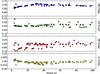 |
Fig. A.2
Difference between JC colour- and S-corrected photometry for NOT (squares), LT (circles), CA 2.2 m (upward triangles), TNG (downward triangles), AS 1.82 m (rightward triangles), AS Schmidt (leftward triangles), TJO (pluses) and FTN (crosses). |
| Open with DEXTER | |
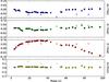 |
Fig. A.3
Difference between SDSS colour- and S-corrected photometry for NOT (squares), LT (circles) and FTN (crosses). |
| Open with DEXTER | |
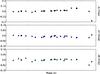 |
Fig. A.4
Difference between 2MASS colour- and S-corrected photometry for NOT (squares), TCS (circles), TNG (upward triangles), CA 3.5 m (downward triangles), WHT (rightward triangles) and LBT (leftward triangles). |
| Open with DEXTER | |
Appendix A.6: Systematic errors
The difference between the S-corrected and colour-corrected JC, SDSS and 2MASS photometry is shown in Figs. A.2–A.4. The differences are mostly less than 5 percent but approaches 10 percent in some cases. Most notably, the difference for the late CA 3.5 m J band observation is ~30 percent because of the strong He 10 830 Å line. So even if the differences are mostly small, S-corrections seems to be needed to achieve 5 percent accuracy in the photometry.
A further check of the precision in the photometry is provided by comparison to the A11, V12, T12, M13, D13, S13 and, in particular, the Swift photometry. The Swift photometry was transformed to the JC system using S-corrections calculated from the Swift filter response functions, which are well known and not affected by the atmosphere. The differences between the JC photometry for all datasets and a spline fit to these observations are shown in Fig. A.5. The systematic (mean) difference for the NOT and LT datasets (which constitutes the bulk of our data) is less than ~5 percent in the B, V, R and I bands and less than ~10 percent in the U band. Considerably larger differences, in the 15–30 percent range, are seen in some datasets, like the A11 WISE 1 m V, R and I, the M13B and V, the D13U and the S13B. The difference between the NOT and LT and the WISE 1m photometry seems to arise partly from differences in the reference stars magnitudes (Iair Arcavi, priv. comm.). As seen in Fig. A.5 as well as in Fig. 1, except for the early (0–40 days) NOT U band observations, the agreement between the NOT, LT and Swift U, B and V band photometry is excellent and the systematic (mean) differences are only a few percent. The early (0–40 days) NOT U band photometry shows a systematic (mean) difference of ~20 percent as compared to the LT and Swift photometry which could be explained by the lack of S-corrections. As the LT filter, in spite of its SDSS nature, is more similar to the JC U band than the NOT filter we favour the LT and Swift photometry in this phase. The good agreement between the NOT and LT JC photometry and the S-corrected Swift JC photometry as well as the bulk of the published JC photometry, gives confidence in the method used. The limited amount of SDSS and 2MASS observations published so far prevents a similar comparison to be done for the SDSS and 2MASS photometry.
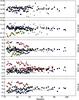 |
Fig. A.5
Difference between JC photometry for the NOT (black squares), LT (black circles), Swift (black upward triangles), A11 (red downward triangles), V12 (green rightward triangles), T12 (blue leftward triangles), M13 (yellow diamonds), D13 (black crosses) and S13 (black pluses) datasets and a cubic spline fit to all these datasets. |
| Open with DEXTER | |
Appendix A.7: Synthetic photometry
Synthetic photometry (used for e.g. S-corrections) was calculated as energy flux based magnitudes in the form  , where Sλ,i and Zi are the energy response function (BM12) and zeropoint of band i respectively. Note that filter response functions are commonly given as photon response functions (BM12) and then have to be multiplied with wavelength to give the energy response functions. JC filter response functions have been adopted from BM12 and zeropoints calculated using the Vega spectrum and JC magnitudes. SDSS filter response functions have been adopted from Doi et al. (2010) and zeropoints calculated using the definition of AB magnitudes (Oke & Gunn 1983) and small corrections following the instructions given at the SDSS site. 2MASS filter response functions have been adopted from Cohen et al. (2003) as provided by the Explanatory Supplement to the 2MASS All Sky Data Release and Extended Mission Products. Swift filter response functions have been adopted from Poole et al. (2008) as provided by the Swift calibration database. To transform the photon count based Swift system into an energy flux based system we have multiplied the response functions with wavelength and re-normalized. The zeropoints were then calculated using the Vega spectrum and Swift magnitudes (Poole et al. 2008). Spitzer filter response functions have been adopted from Hora et al. (2008) as provided at the Spitzer web site and zeropoints calculated using the Vega spectrum and Spitzer magnitudes.
Appendix A.8: Swift UV read leak
The response functions of the Swift UVW1 and UVW2 filters (Poole et al. 2008) have a quite strong red tail. If, as is often the case for SNe, there is a strong blueward slope of the spectrum in the UV region this will result in a red leakage that might even dominate the flux in these filters. In Fig. A.6 we quantify this by showing the fractional red leakage defined as the fractional flux more than half the equivalent width redwards of the mean energy wavelengths of the filters. The spectrum was interpolated from the photometry as explained in Sect. 3.3 excluding the UVW1 and UVW2 filters. After ~20 days the leakage is ~80 and ~60 percent in the UVW1 and UVW2 filters respectively. Given this the UVW1 and UVW2 lightcurves do not reflect the evolution of the spectrum at their mean energy wavelengths and we will therefore exclude these from our analysis.
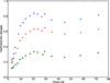 |
Fig. A.6
Fractional red leakage in the Swift UVW1 (red circles), UVM2 (green squares) and UVW2 (blue triangles) filters. |
| Open with DEXTER | |
Appendix B: Progenitor observations
We have obtained high quality pre- and post-explosion B, V and r band images of the SN site with the NOT. The pre-explosion images were obtained on May 26 2008 (B) and May 29 2011 (V and r), the latter just 2 days before the explosion. Two sets of post-explosion images were obtained, the first on Jan. 20 2013 (V and r) and Mar. 19 2013 (B), 601 and 659 days post explosion respectively, and the second on Apr. 14 2013 (V), May 15 2013 (r) and June 1 2013 (B), 685, 715 and 732 days post explosion respectively. In Fig. B.1 we show a colour composite of the pre-explosion and the second set of post-explosion B, V and r band images where the RGB values have been scaled to match the number of photons. The photometry presented below have been calibrated to the natural Vega (BV) and AB (r) systems of the NOT using the reference star magnitudes and colour constants presented in this paper (Tables A.5, A.7, A.2 and A.3).
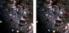 |
Fig. B.1
Colour composite of the pre- (left panel) and post- (right panel) explosion NOT imaging. The RGB values have been scaled to match the number of photons. |
| Open with DEXTER | |
We have used the HOTPANTS package to perform subtractions of the pre- and post-explosion images and aperture
photometry to measure the magnitudes of the residuals to B = 23.00 ± 0.10, V = 22.73 ± 0.07 and r = 22.22 ± 0.05 mag for the first set of post-explosion observations and B = 22.73 ± 0.06, V = 22.23 ± 0.05 and r = 21.95 ± 0.04 mag for the second set of post-explosion observations. The positions of the residuals in all bands are within 0.15 arcsec from the position of the SN. The two fainter nearby stars, seen in pre-explosion HST images, that could possibly contaminate the result are ~0.5 arcsec away from the SN so their contribution (due to variability) to the residuals is likely to be small. Using PSF photometry where we have iteratively fitted the PSF subtracted background we measure the magnitudes of the yellow supergiant in the pre-explosion images to B = 22.41 ± 0.12, V = 21.89 ± 0.04 and r = 21.67 ± 0.03 mag. The residuals for the second set of post-explosion observations then corresponds to a reduction of the flux with 74 ± 9, 73 ± 4 and 77 ± 4 percent in the B, V and r bands respectively. The remaining flux, at least partly emitted by the SN, corresponds to B = 23.35 ± 0.32, V = 22.56 ± 0.10 and r = 22.67 ± 0.11 mag for the first set of post-explosion observations and B = 23.89 ± 0.50, V = 23.32 ± 0.20 and r = 23.28 ± 0.19 mag for the second set of post-explosion observations.
© ESO, 2014
Current usage metrics show cumulative count of Article Views (full-text article views including HTML views, PDF and ePub downloads, according to the available data) and Abstracts Views on Vision4Press platform.
Data correspond to usage on the plateform after 2015. The current usage metrics is available 48-96 hours after online publication and is updated daily on week days.
Initial download of the metrics may take a while.