| Issue |
A&A
Volume 560, December 2013
|
|
|---|---|---|
| Article Number | A79 | |
| Number of page(s) | 15 | |
| Section | Astrophysical processes | |
| DOI | https://doi.org/10.1051/0004-6361/201322266 | |
| Published online | 09 December 2013 | |
Online material
Appendix A: Numerical scheme for RAMSES-RHD
This Appendix provides the Jacobian matrices and their eigenstructure for reconstructing the primitive variables in the 3D-RHD case. It also explains the recovery of the primitive variables.
Appendix A.1: Recovering the primitive variables
To determine the primitive variables (ρ,vj,P)T, we simplify the method by Mignone & McKinney (2007), initially developed for relativistic magnetohydrodynamics. One rewrites the total energy  (A.1)and solves an equation on W′ = W − D = ρhΓ2 − ρΓ.
To avoid numerical problems in the non-relativistic or ultrarelativistic limits, one introduces  (A.2)such that the Lorentz factor is given by
  (A.3)This gives
  (A.4)which can be used to replace P in Eq. (A.1). Once W′ is found using, say, a Newton-Raphson method, one recovers the Lorentz factor using Eqs. (A.2) and (A.3), then the density ρ = D/Γ and finally pressure using Eq. (A.4). We determine W′ with a precision of 10-10.
The method can be easily adapted to different equations of state, by simply changing Eq. (A.4). It is well suited to codes with AMR since an initial guess of the value of W0, which guarantees the positivity of pressure, can be found analytically (Mignone & McKinney 2007). This avoids storing values of W′ between time steps, which can be cumbersome on a changing grid. One can determine W0, which then gives  , rewriting the pressure as
 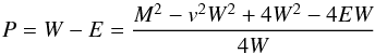 (A.5)since M2 ≡ W2v2. Pressure is thus guaranteed to be positive when
  (A.6)This happens for any W > W+, with W+ the largest of the two roots of the quadratic equation Eq. (A.6). As v < 1, solving Eq. (A.6) for v = 1, implies that the corresponding root W+ ,1 > W+ ,v, which guarantees positive pressure. One thus uses W+ ,1 as the initial guess to start the Newton-Raphson scheme.
Provided the vector of conservative variables is physical, this method converges to a physical primitive state. The positivity of the density can be verified by D > 0. Subluminal velocity is guaranteed by E2 > M2 + D2. Indeed, using Eq. (6) one has 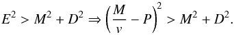 (A.7)This necessarily implies positive pressure and v < 1. Whenever a non-physical conserved state occurs, we floor the density to ρ = 10-10 and the pressure to P = 10-20. This occurs roughly once every 106 updates in our gamma-ray binary simulations. It occurs in the unshocked pulsar wind, where the density and pressure are lowest and the Lorentz factor the highest. It mostly occurs along the line of centers of the binary, since the Cartesian grid is unable to perfectly model the spherical symmetry of the wind. The number of failures strongly reduces with resolution. Beckwith & Stone (2011) note a few failures when pressure is very low and suggest using the entropy instead of the energy as conserved variable in those cases. Reconstruction by using the neighbouring cells is very cumbersome owing to the AMR structure in RAMSES, so we have not considered this option.
Appendix A.2: Computing the time step
The time step is determined by the Courant condition for unsplit schemes 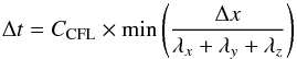 (A.8)where CCFL is the Courant number and λk is the propagation speed along direction k determined by
 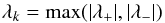 (A.9)with
 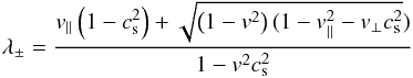 (A.10)where v∥ and v⊥ are the velocity parallel and perpendicular to the direction k. All the simulations in this paper were performed using CCFL = .8.
Our determination of the time step is more restrictive than the more commonly used (see e.g. Mignone et al. 2012) 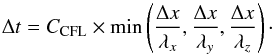 (A.11)Using the above expression for the time step, we find that the simulation of the 3D jet (Appendix B.3) shows no failure for CCFL ≤ .5, which is comparable to other codes (Zhang & MacFadyen 2006).
Appendix A.3: Jacobian matrices of the 3D-RHD equations
This section will only be available online. One has 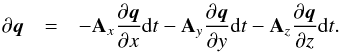 (A.12)Following Font et al. (1994) for a 1D flow with transverse velocity and the general definition of the enthalpy
 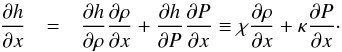 (A.13)With these definitions, the sound speed can be written as
 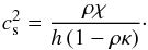 (A.14)For the classical equation of state, one has
 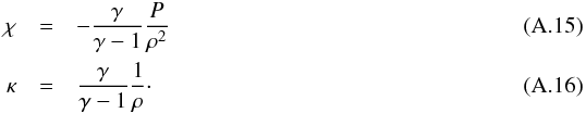 The complete Jacobian matrix is given by
 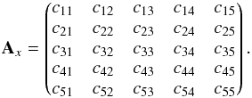 (A.17)
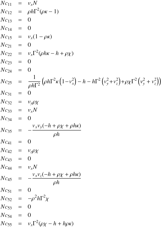 with N = ( − h + hρκ + ρχv2)Γ2.
The matrix Ay is given by 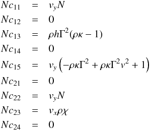
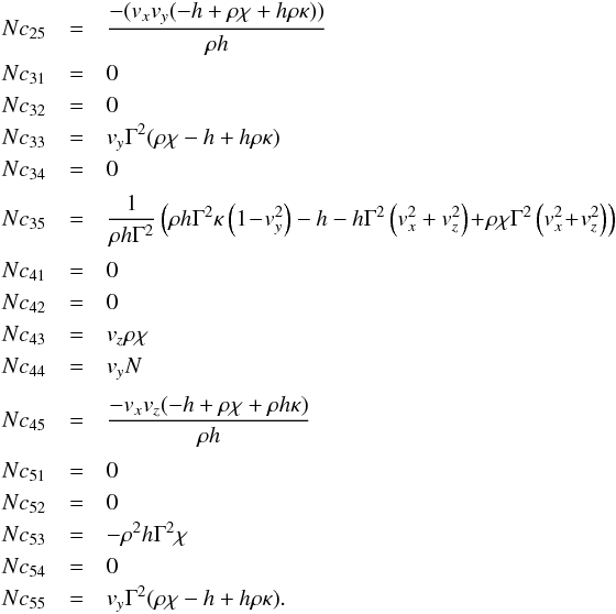 Along z one has Az given by
Appendix A.4: Eigenstructure
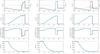 |
Fig. B.1
Density, AMR levels (red dashed line), parallel and transverse velocity and pressure in the frame of the laboratory for the shock test with Γmax = 120. Left panels: uniform grid nx = 512; middle panels: uniform grid nx = 217 = 131072; right panels: nx = 64, lmax = 17. The black solid line represents the MUSCL method, while the black dashed line represents the PLM method. At high resolution, they give the same result, which is very close to the analytic solution. |
| Open with DEXTER | |
The eigenvalues of Ax are (see e.g. Falle & Komissarov 1996) 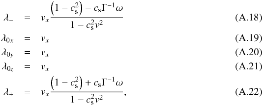 with
with  (A.23)The left eigenvectors are given by
 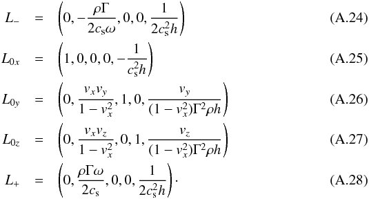 The right eigenvectors are given by
 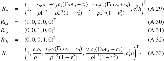 Similarly for Ay one has
 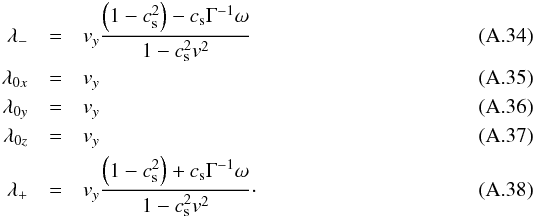 with
with  (A.39)The left eigenvectors are given by
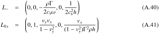
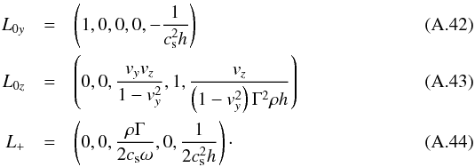 The right eigenvectors are given by
 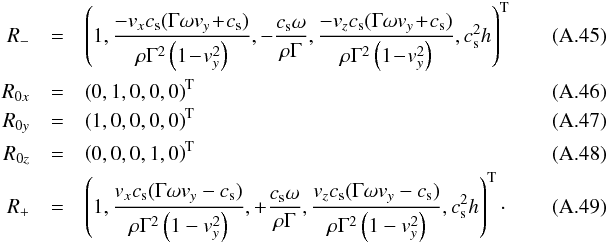 For Az one has
 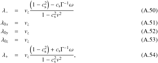 with
with  (A.55)The left eigenvectors are given by
  The right eigenvectors are given by
Appendix B: Numerical tests
In this section, we present a set of numerical tests that validate our new relativistic code. Unless stated differently, all the simulations were performed with Courant number CCFL = 0.8, the minmod slope limiter in the MUSCL scheme and for the AMR prolongations, and the HLLC Riemann solver. The adiabatic index is set to 5/3. Refinement is based on density and velocity gradients.
Appendix B.1: 1D Sod test
One initially starts with two different media separated by an interface located at x = 0.5. When the simulation begins, the interface is removed and the flow evolves freely following a self-similar structure. The flow decays into three waves, usually a rarefaction, a contact discontinuity, and a shock. These tests are very common because easy to implement and comparisons with analytic solutions are possible (see Martí & Müller 1994, for pioneering work; and Rezolla et al. 2003, for an elegant version including transverse velocities).
We reproduce the test of Sect. 2.3, with a maximal Lorentz factor of 120. Contrary to the Newtonian case, transverse velocities do impact the shock structure in RHD and reduce the shock velocity. Several groups have shown that tests with high transverse velocities are very stringent and only show satisfactory results at very high resolution (Mignone & Bodo 2005; Zhang & MacFadyen 2006).
Figure B.1 gives the density, parallel, and transverse velocity and pressure at tend = 1.8 for tests with different resolutions. The thick black line represents the simulation using the MUSCL scheme with the minmod limiter while the dashed line represents the simulation following the PLM method with the moncen limiter. Both methods lead to similar results. The AMR levels are superposed on the density plots. Refinement is based on the gradients of both the Lorentz factor and pressure. The first simulation has a uniform resolution of 512 cells, which is close to the resolution used by Mignone et al. (2005). Our simulation is similar to theirs, with the shock running ahead of its theoretical position and some inaccuracy in the orientation of the velocity vector. These discrepancies reduce with increasing resolution. In the second simulation, the resolution is also uniform but set to 217 = 131 072 cells. This is the same resolution as Ryu et al. (2006), and we obtain very good agreement with their results and the analytic solution. At high resolution, there is no clear difference between the PLM and MUSCL method. However, such high resolution is prohibitive in multidimensional simulations. The last panel shows a simulation with AMR, the coarse level is set by nx = 64, while the highest level lmax = 17. The result is in very good agreement with the expected solution. The density difference between our results and the analytic solution is lower than one percent, even at the discontinuities. At the end of the test, the gain of computing time is about a factor 200 compared to the uniform grid. A simulation with the same computing time, but on a uniform grid would have a resolution of slightly more than 4096 cells. A test simulation with a uniform resolution nx = 4096 showed a 40% discrepancy in the density at the beginning of the shocked region, with respect to the analytic solution. AMR proves to be very helpful tool in the modelling of highly relativistic flows.
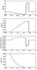 |
Fig. B.2
Inclined shock test: density, velocity, pressure and Lorentz factor along the shock normal. The thick solid lines give the 2D results, the dot-dashed lines the 1D results from a simulation with the same resolution, and the blue lines give the analytic solution. The resolution is lower than for the 1D test in Sect. B.1. |
| Open with DEXTER | |
Appendix B.2: 2D Inclined shock tube
Two-dimensional tests are important to verify the accuracy of the coupling between the different components of the four-vectors. We performed the above Sod tests by inclining the interface between the two media by θ = 21.7° with respect to a vertical line. The value of θ is chosen arbitrarily to avoid any peculiar alignement with respect to the numerical grid, as could occur for θ = 45° (Radice & Rezzolla 2012). Since the initial separation between both sides is inclined, for a given y, the initial conditions are shifted by a few cells with repect to the row of cells just below. The boundary conditions along the y axis follow the same shift. At the bottom boundary one has  (B.1)for all the cells with i − nshift = i − (ny × tanθ) > 0. The boundary conditions are periodic along the x axis. The simulations took 2200 CPU hours.
The simulations should give a comparable result to 1D simulations with the same resolution. Figure B.2 shows the different variables in the direction normal to the shock for the second test using a 12 800 × 6400 uniform resolution. The given values were obtained by performing a bilinear interpolation of the 2D simulation. We overplot the analytic solution and the result from a 1D simulation with the same resolution along the interface between the flows (ny/cosθ = 6400 cells). The 2D simulation differs somewhat from its equivalent 1D simulation. This suggests that direct comparison between unidimensional and multidimensional simulations is not possible and that, for high Lorentz factors, multidimensional simulations need a higher resolution to be numerically accurate.
In both the 1D and the 2D simulations, the position of the shock is ahead of its theoretical position. The 1D and 2D tests have shown that this effect weakens at higher resolution.
Appendix B.3: 3D jet
Relativistic jets have become a widespread way to test multidimensional RHD codes. Their complex dynamics show the impact of transverse velocities and display the development of instabilities. In this case, no analytic solution exists, and validation is done by comparison with former results. We follow the setup by Del Zanna & Bucciantini (2002) The length scale is given by the initial radius of the jet r0 = 1, the size of the box is 20r0, with lmin = 6 and lmax = 9. This gives an equivalent resolution of 25 cells per radius, while the original test was performed with a resolution of 20 cells per radius. We perform a 3D simulation, while most jets are simulated using axisymmetric 2D simulations (Lucas-Serrano et al. 2004). Except at the injection of the jet, we use outflow boundary conditions. The maximum Lorentz factor is 7.1. The evolution of the density profile is given in Fig. B.3. One can see the typical features of relativistic jets: the bow shock with the external medium, the cocoon of shocked medium, the relativistic beam, and the Mach disk. The Kelvin-Helmholtz instability develops at the interface between the shocked external medium and the shocked material from the jet. The overall shape is similar to the simulation by Del Zanna & Bucciantini (2002) although the simulation with RAMSES-RHD presents a small extension at the head of the jet. This is due to the carbuncle instability (Peery & Imlay 1988), which arises when cylindrical or spherical phenomena are simulated on a Cartesian grid. Performed on 16 processors, this simulation took 320 mono-CPU hours. The same simulation on a 5123 fixed grid took about 500 h. Owing to the complex structure inside the jet, AMR is not very efficient in this type of simulation (Zhang & MacFadyen 2006).
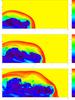 |
Fig. B.3
Simulation of the propagation of a 3D relativistic jet (Γmax = 7.1). From top to bottom: density at t = 20,30,40 in a 3D jet starting from the left boundary of the domain. |
| Open with DEXTER | |
© ESO, 2013
Current usage metrics show cumulative count of Article Views (full-text article views including HTML views, PDF and ePub downloads, according to the available data) and Abstracts Views on Vision4Press platform.
Data correspond to usage on the plateform after 2015. The current usage metrics is available 48-96 hours after online publication and is updated daily on week days.
Initial download of the metrics may take a while.