| Issue |
A&A
Volume 560, December 2013
|
|
|---|---|---|
| Article Number | A79 | |
| Number of page(s) | 15 | |
| Section | Astrophysical processes | |
| DOI | https://doi.org/10.1051/0004-6361/201322266 | |
| Published online | 09 December 2013 | |
Simulating gamma-ray binaries with a relativistic extension of RAMSES⋆
1 UJF-Grenoble 1 / CNRS-INSU, Institut de Planétologie et d’Astrophysique de Grenoble (IPAG) UMR 5274, 38041 Grenoble, France
e-mail: This email address is being protected from spambots. You need JavaScript enabled to view it.
2 Physics Department, University of Wisconsin-Milwaukee, Milwaukee WI 53211, USA
3 Laboratoire AIM, CEA/DSM - CNRS - Université Paris 7, Irfu/Service d’Astrophysique, CEA-Saclay, 91191 Gif-sur-Yvette, France
4 Institute for Theoretical Physics, University of Zürich, Winterthurestrasse 190, 8057 Zürich, Switzerland
Received: 11 July 2013
Accepted: 29 September 2013
Abstract
Context. Gamma-ray binaries are composed of a massive star and a rotation-powered pulsar with a highly relativistic wind. The collision between the winds from both objects creates a shock structure where particles are accelerated, which results in the observed high-energy emission.
Aims. We want to understand the impact of the relativistic nature of the pulsar wind on the structure and stability of the colliding wind region and highlight the differences with colliding winds from massive stars. We focus on how the structure evolves with increasing values of the Lorentz factor of the pulsar wind, keeping in mind that current simulations are unable to reach the expected values of pulsar wind Lorentz factors by orders of magnitude.
Methods. We use high-resolution numerical simulations with a relativistic extension to the hydrodynamics code RAMSES we have developed. We perform two-dimensional simulations, and focus on the region close to the binary, where orbital motion can be neglected. We model different values of the Lorentz factor of the pulsar wind, up to 16.
Results. We determine analytic scaling relations between stellar wind collisions and gamma-ray binaries. They provide the position of the contact discontinuity. The position of the shocks strongly depends on the Lorentz factor. We find that the relativistic wind is more collimated than expected based on non-relativistic simulations. Beyond a certain distance, the shocked flow is accelerated to its initial velocity and follows adiabatic expansion. Finally, we provide guidance for extrapolation towards more realistic values of the Lorentz factor of the pulsar wind.
Conclusions. We extended the adaptive mesh refinement code RAMSES to relativistic hydrodynamics. This code is suited to studying astrophysical objects, such as pulsar wind nebulae, gamma-ray bursts, or relativistic jets, and will be part of the next public release of RAMSES. Using this code we performed simulations of gamma-ray binaries up to Γp = 16 and highlighted the limits and possibilities of current hydrodynamical models of gamma-ray binaries.
Key words: hydrodynamics / relativistic processes / methods: numerical / X-rays: binaries / gamma rays: stars
Appendices are available in electronic form at http://www.aanda.org
© ESO, 2013
1. Introduction
Composed of a massive star and a compact object, gamma-ray binaries emit most of their power at GeV and TeV energies. Up to now a handful of such systems have been detected: PSR B1259-63 (Aharonian et al. 2005b), LS 5039 (Aharonian et al. 2005a), LSI +61°303 (Albert et al. 2006), and more recently 1FGL J1018.6-5856 (Fermi LAT Collaboration et al. 2012) and HESS J0632+057 (Bongiorno et al. 2011).
Pulsed radio emission in PSR B1259-63 (Johnston et al. 1992) indicates the compact object is a fast-rotating pulsar, while the nature of the compact object in the other systems is less certain. In PSR B1259-63 the high-energy emission probably arises from the interaction between the relativistic wind from the pulsar and the wind from the companion star (Tavani et al. 1994). It displays extended radio emission showing a structure looking like a cometary tail whose orientation changes with orbital phases (Moldón et al. 2011a). It is interpreted as the evolution of a shock as the pulsar orbits around the massive star. The similarities in the variable high-energy emission and the extended radio emission between PSR B1259-63 and the other detected gamma-ray binaries suggest the wind collision scenario is at work in all the systems (Dubus 2006).
These binaries share a common structure with colliding wind binaries composed of two massive stars. Colliding stellar winds have been extensively studied in the past few years using numerical simulations (see e.g. Parkin et al. 2011) that have highlighted the importance of various instabilities in the colliding wind region. The Kelvin-Helmholtz instability (KHI) can have a strong impact, especially when the velocity difference between the winds is important. Lamberts et al. (2012, hereafter Paper II) show that it may destroy the expected large scale spiral structure. However, strong density gradients have a stabilizing effect. For strongly cooling winds, the shocked region is very narrow and the non-linear thin shell instability (Vishniac 1994) can strongly distort it (Lamberts et al. 2011, hereafter Paper I). For highly eccentric systems, the instability may grow only at periastron, where the higher density in the collision region leads to enhanced cooling (Pittard 2009). A very high resolution is required to model this instability, and up to now large scale studies have been limited by their numerical cost.
Both these instabilities create a turbulent colliding wind region, and may be responsible for the variability observed in stellar colliding wind binaries. They can distort the positions of the shocks, thereby shifting the location of particle acceleration. Strong instabilities also lead to a significant amount of mixing between the winds (Paper II). This may enhance thermalization of non-thermal particles and decrease their high-energy emission. All these effects may be at work in gamma-ray binaries to affect their structure and emission properties (Bosch-Ramon & Barkov 2011; Bosch-Ramon et al. 2012).
The first numerical studies of the interaction between pulsar winds and their environment were performed in the hydrodynamical limit (van der Swaluw et al. 2003; Bucciantini 2002). While providing good insight into the overall structure, a relativistic temperature or bulk motion of the plasma can have subtle effects. For instance, the normal and transverse velocities are coupled via the Lorentz factor even for a normal shock. The specific enthalpy of a relativistic plasma is also greater than for a cold plasma. A relativistic treatment is also necessary for estimating the impact of Doppler boosting on emission properties of the flow. Relativistic simulations have studied the morphology of the interaction between pulsar winds and supernova remnants (Bucciantini et al. 2003), the interstellar medium (Bucciantini et al. 2005), or the wind of a companion star (Bogovalov et al. 2008). Studies have focussed on the impact of magnetization and anisotropy in the pulsar wind or orbital motion (Vigelius et al. 2007; Bogovalov et al. 2012). They also provide models for non-thermal emission from pulsar wind nebulae (Del Zanna et al. 2006; Volpi et al. 2008; Komissarov & Lyubarsky 2004).
One of our goals is to determine the importance of relativistic effects both on the structure and stability of gamma-ray binaries. We perform a set of 2D simulations of gamma-ray binaries and study the impact of the momentum flux ratio and the Lorentz factor of the pulsar wind on the colliding wind region. We also determine the impact of the Kelvin-Helmholtz instability on the colliding wind region (Sect. 3). We therefore extend the hydrodynamics code RAMSES to special relativistic hydrodynamics (Sect. 2). We explain the implementation within the AMR scheme in particular and present some tests (Appendix A) that validate this new code for relativistic hydrodynamics. We discuss how our results can be extrapolated to more realistic values for the Lorentz factor of the pulsar wind (Sect. 4) and conclude (Sect. 5).
2. Relativistic hydrodynamics with RAMSES
RAMSES (Teyssier 2002) is a numerical method for multidimensional astrophysical hydrodynamics and magnetohydrodynamics (Fromang et al. 2006). RAMSES uses an upwind second-order Godunov method. The vector of conserved variables U is averaged over the volume of the cells and fluxes F at cell interfaces are averaged in time. The updates in time are then given by 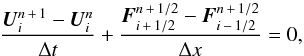 (1)where the subscript i stands for the index of the cell and n refers to the time step.
RAMSES uses a Cartesian grid and allows the use of adaptive mesh refinement (AMR), which enables the resolution to be locally increased at a reasonable computational cost.
2.1. Equations of relativistic hydrodynamics (RHD)
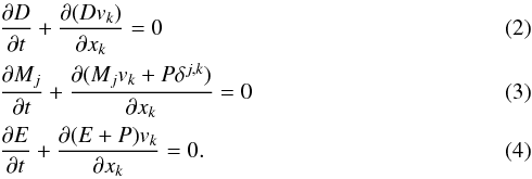
Throughout this paper the speed of light is c ≡ 1. In the frame of the laboratory, the 3D-RHD equations for an ideal fluid can be written as a system of conservation equations (Landau & Lifshitz 1959).
 These equations can be expressed in compact form
 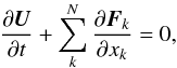 (5)where the vector of conservative variables is given by
 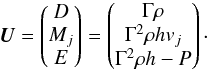 (6)The fluxes Fk along each of the N directions are given by
 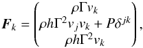 (7)where D is the density, M the momentum density, and E the energy density in the frame of the laboratory. The subscripts j,k stand for the dimensions, δjk is the Kronecker symbol, and h is the specific enthalpy given by
  (8)and ρ is the proper mass density, vj the fluid three-velocity, P the gas pressure, and e is the sum of the internal energy and rest mass energy of the fluid. The Lorentz factor is given by
  (9)A passive scalar s can be included in the simulations using S = sρΓ as the conserved variable and F = ρsvΓ to compute its flux.
An equation of state closes the system of Eqs. (2)–(4). The most commonly used is the so-called classical equation of state, where the rest mass energy is removed from the total internal energy e:  (10)where γ is the ratio of specific heats (or adiabatic index), which is constant and should not be confused with the Lorentz factor Γ. In the non-relativistic limit γ = 5/3, in the ultrarelativistic limit γ = 4/3. The sound speed is given by
 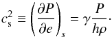 (11)This leads to cs < 1/3 in the ultrarelativistic limit and cs < 2/3 in the non-relativistic limit. The kinetic theory of relativistic gases (Synge 1957) shows that the ratio of specific heats cannot be kept constant when passing from non-relativistic to highly relativistic temperatures and provides an equation of state that is valid for all temperatures. Owing to the complexity of the expressions relating different thermodynamical quantities, approximations have been developed for the implementation in numerical schemes (Falle & Komissarov 1996; Mignone et al. 2005; Ryu et al. 2006; Mignone & McKinney 2007). This has not been implemented yet in the relativistic extension of RAMSES that we present.
The RHD equations have a similar structure to the Euler equations and can be solved following the same numerical method and making only localized changes. Still, the strong coupling of the equations through the presence of the Lorentz factor and the enthalpy makes the resolution of the equations more complex. Moreover, in relativistic dynamics, velocities are bounded by the speed of light, resulting in an important numerical constraint. These changes particularly affect the determination of the primitive variables, the development of a second-order scheme (Sect. 2.2), and the AMR framework (Sect. 2.3).
2.2. Second-order numerical scheme
Several steps in the algorithm require the use of the primitive variables  (12)In classical hydrodynamics, analytic relations allow a straightforward conversion from conservative to primitive variables. In RHD, there are no such relations, and several methods have been developed to recover the primitive variables (see e.g. Aloy & Martí 1999; Noble et al. 2006; Ryu et al. 2006). We use the method described in Mignone & McKinney (2007), which uses a Newton-Raphson algorithm to solve an equation on W′ = W − D = ρhΓ2 − ρΓ. The details of the computation are given in Appendix A.1.
The determination of the fluxes F cells in Eq. (1) involves solving the Riemann problem at the interface between cells. Different solvers have been developed, and some have been extended to RHD. We have implemented the relativistic HLL and HLLC solver in RAMSES. For the HLL Riemann solver, the expression of the Godunov flux is identical to the non-relativistic expression (Schneider et al. 1993). However, the computation of the maximal wavespeeds propagating towards the left and right is different. In Newtonian hydrodynamics, the wavespeed is the sum of the sound speed and the advection speed of the flow. The relativistic composition of velocities couples the velocity of the flow parallel and perpendicular to the direction of spatial derivation and all components of the velocity need to be taken into (Del Zanna & Bucciantini 2002). An HLLC solver was developed by Mignone & Bodo (2005), whose method we closely follow.
To reach high enough accuracy in scientific applications, second-order schemes are, however, necessary. In such cases, fluxes are determined half a time step ahead of the current time step. We have implemented the monotonic upstream scheme for conservation laws (MUSCL) and piecewise linear (PLM) methods. In both schemes, the update is performed on the primitive variables, which are determined by a Taylor expansion 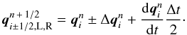 (13)The subscripts L and R respectively stand for the left-and right-hand sides of a cell boundary,
  are the slopes of the variables in the cell, computed using a slope limiter, which is not affected by special relativity,
  is the temporal variation, given by
 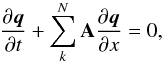 (14)where A = ∂F(q)/∂U(q) is the Jacobian matrix of the system. In classical hydrodynamics, flows in a given direction are not affected by motions perpendicular to that direction. In RHD all spatial directions are coupled through the Lorentz transformation: A is 5 × 5 matrix even for 1D flows (Pons et al. 2000). The value of A and its equivalents along the y and z directions are given in Appendix A.3.
In a MUSCL-Hancock scheme (Van Leer 1979), one uses 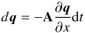 (15)directly to reconstruct the variables. In RAMSES, we have found that this reconstruction gives satisfactory results with the minmod (Roe 1986) slope limiter but fails with the moncen limiter (van Leer 1977). Therefore we implemented the PLM method, which works with both limiters.
In the Piecewise Linear Method (Collela 1990), one rewrites Eq. (14) 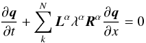 (16)with λα the eigenvalues, and (Lα,Rα) the eigenvectors of the Jacobian matrix. In this case, the slopes are projected on the characteristic variables, using the left-hand eigenvectors. The waves that cannot reach the interface between cells in the given time step are filtered out and do not contribute to the interface states. One then recovers the primitive variables, multiplying by the right-hand eigenvectors. The final interface states are then computed by adding the contributions of all the selected waves:
 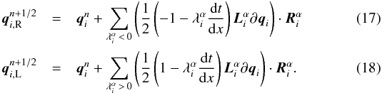 The full set of eigenvalues and eigenvectors is given in Appendix A.3.
Since all directions are reconstructed separately, although each component is subluminal, nothing guarantees that the norm of the total velocity remains subluminal. When a superluminal velocity is obtained, one possibility is to reconstruct Γv and renormalize the velocity when necessary (Aloy & Martí 1999) or to reconstruct the Lorentz factor independently (Wang et al. 2008). When superluminous velocities are obtained, we choose to switch to first-order reconstruction (qi ± 1/2,L,R = qi) in all directions, for all variables. No switch occurred in our test simulation of a relativistic jet (see Sect. B.3). It typically occurs once every 107 updates in our gamma-ray binary simulations with a Lorentz factor of 7, probably due to the much larger region covered by the high-velocity flow and its very low pressure (see Sect. 3.3).
Figure 1 shows the result of a shock tube test for the two different methods. Both methods give comparable results and show that the code works well on a uniform grid. In this test (Martí & Müller 2003), ρL = 10, ρR = 1, PL = 13.3 and PR = 10-6 and there is no initial velocity. The flow is only mildly relativistic in the dynamical sense but e ≫ ρ in the right-hand state, resulting in a thermodynamically highly relativistic flow. Figure 2 illustrates the differences between a non-relativistic adiabatic index (γ = 5/3) and the ultrarelativistic adiabatic index (γ = 4/3). The compression ratio in the shocked region is higher than for Newtonian hydrodynamics, especially when the gas is thermodynamically ultrarelativistic. The results compare very well with Fig. 2 in Ryu et al. (2006).
 |
Fig. 1 Density, velocity, and pressure in the laboratory frame at t = 0.45. The thin solid line shows the PLM method, the dashed line the MUSCL metod, which gives very similar results. The analytic solution (Giacomazzo & Rezzolla 2006) is given in blue. The resolution is nx = 256. |
 |
Fig. 2 Density, velocity, and pressure in the laboratory frame at t = 0.45 for tests with different adiabatic indices. The black solid line shows γ = 5/3, the dashed green line shows γ = 4/3, the resolution is nx = 256. |
2.3. Implementation within the AMR structure
Mesh refinement is an important tool when modelling a wide range of spatial structures. Several methods exist and have been successfully associated with RHD schemes: static mesh refinement (Beckwith & Stone 2011), block-based AMR (Hughes et al. 2002; Zhang & MacFadyen 2006; Mignone et al. 2012) or tree-based AMR as in Keppens et al. (2012). Moving meshes offer another possibility to enable locally increased resolution (Duffell & MacFadyen 2011).
In RAMSES, cells are related in a recursive tree structure (Kravtsov et al. 1997) and gathered together in octs of 2N cells (N is the number of dimensions), which share the same parent cell. When creating new refined cells or computing the fluxes at the interface between two levels, the conserved variables need to be interpolated from level l to level l + 1. The interpolation is done at second order, using a minmod limiter for the linear reconstruction. Conversely, since hydrodynamical updates are only performed at the highest level of refinement, variables need to be determined at lower levels by computing the average over the whole oct.
In RHD, the restriction step may lead to failures, when the energy is strongly dominated by the kinetic energy. In RHD, positive pressure and subluminal velocity are guaranteed when E2 > M2 + D2 (Mignone & Bodo 2005, see Appendix A for the demonstration). Although cells at a given level satisfy this condition, nothing guarantees that  where the subscript oct means variables are summed over an oct. The resulting state can be non-physical. We found that this problem can be bypassed by performing the reconstruction on the specific internal energy ϵ (i.e. the temperature) rather than on the total energy using
  (19)where P and ρ are computed with the Newton-Raphson scheme used to computed the primitive variables. After the restriction, one recovers the total energy using
  (20)where
  (21)This method makes the numerical scheme non-conservative but guarantees that the pressure is positive and the speed is subluminal.
Refinement is often based on gradients in the flow variables: either the density, pressure or velocity. In highly relativistic flows, the velocity does not vary significantly and the variations in the Lorentz factor may not be captured properly, thus strongly altering the dynamics of highly relativistic flows. To avoid this, we have implemented refinement based on the gradients of the Lorentz factor. Figure 3 shows two simulations of a shock tube test. We reproduced the test by Pons et al. (2000), with ρL = ρR = 1, PL = 103, and PR = 10-2, vx,L = vx,R = 0, vy,L = vy,R = 0.99 initially. This is a very stringent test, with a maximum Lorentz factor of 120. In the first case, refinements are only based on pressure gradients and do not properly capture the contact discontinuity and positions of the shock. In the other simulation, refinement is also based on the Lorentz factor. In this case, the simulation is in very good agreement with the analytic result. Similar accuracy can also be found by refining according to both the pressure and density gradients. However, it increases the computational cost by ≃15% in this test. This test validates the implementation within the AMR framework, which is well adapted for shocks in highly relativistic flows. We estimated the level in non-conservation by measuring the variation of the total density, momentum, and energy (in the laboratory frame) at the end of the test. We found relative errors of 3 × 10⁻⁹, 9 × 10⁻⁵, and − 6 × 10⁻⁸, respectively.
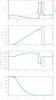 |
Fig. 3 Density, parallel velocity, transverse velocity, and pressure in the laboratory frame for two different simulations. In both cases, the coarse grid is set by nx = 64 with 11 levels of refinement based on pressure gradients. The solid line shows a simulation where additional refinements occur based on Lorentz factor gradients. The result is superimposed to the analytic solution (Giacomazzo & Rezzolla 2006) given in blue. The red dashed line in the upper panel shows the refinement levels, based on the Lorentz factor gradients. |
This method is currently implemented in RAMSES and succesfully passes all the commonly used numerical tests. A few of them are detailed in Appendix B.
3. 2D simulations of gamma-ray binaries
Pulsar winds have a Lorentz factor of about 104 − 106 (see e.g. Kirk et al. 2009, for a review), which is far beyond the reach of current computer power and numerical schemes. Most present multidimensional simulations model Lorentz factors of at most a few 10. Modelling higher Lorentz factors, especially in low-density or low-pressure environments, require highly sophisticated numerical methods, particularly in 2D and 3D, since spatial directions are strongly coupled. Up to now, there has been no extensive study of the impact of relativistic effects regarding the interaction of a pulsar wind with its surroundings.
The following simulations are demanding, not only because they need high resolution, but also because of the different timescales involved. The longest dynamical time is set by the speed of the stellar wind, while the time step in the simulation is limited by the speed of the pulsar wind. Because vp/v∗ ≃ 100, simulating a gamma-ray binaries takes roughly a hundred times longer than simulating colliding stellar winds. The simulations in this section typically took between 10 000 and 15 000 CPU hours to complete.
3.1. Collision with supersonic relativistic winds
We have compared the interaction between a pulsar wind and a stellar wind to the collision between two stellar winds descried in Paper I. Similarly to the non-relativistic case, one can determine the position of the contact discontinuity between the winds. The standoff point, which is situated at the intersection between the line-of-centres and the contact discontinuity, is given by the equation of momentum fluxes 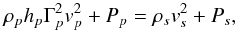 (22)where the subscript s represents the variables in the stellar wind, and the variables with subscript p refer to the pulsar. We neglect thermal pressure in the winds, which gives
 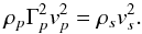 (23)The mass loss rate Ṁ ≡ 4πr2Γρv is constant so the location of standoff point, where Eq. (22) is realized, is set by the dimensionless ratio
 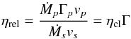 (24)where ηcl (Stevens et al. 1992) is the usual definition of the momentum flux ratio of the winds in the non-relativistic limit. These equations suggest that we can expect a similar structure to the one in colliding stellar winds, provided we define the momentum flux ratio of the winds using Eq. (24).
3.2. Numerical setup
We performed 2D numerical simulations of the interaction in a region extending up to four times the binary separation a. Our 2D setup is cylindrical, as described in Paper I. We neglected orbital motion in our simulations to enable comparisons with the analytic estimates and clarify the differences with our previous non-relativistic results (Paper I). Orbital motion can be neglected without affecting the dynamics on scales much smaller than the spiral stepsize S ≳ vsPorb (Paper II). For LS 5039, the gamma-ray binary with the shortest known period, the step of the spiral is at least S ≃ 4 AU, which about 20 times the binary separation (Moldón et al. 2012).
Since we want to study the impact of relativistic effects, we do not set the pulsar wind velocity to ≃c but keep it as a free parameter. We set ηrel and vp and derive the pulsar’s mass loss rate 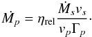 (25)As for the classical case, the winds are initialized in masks following the method described in Lemaster et al. (2007). Density is determined by mass conservation in the winds, and the velocity is set to the terminal velocity. As in stellar wind simulations, we set the Mach number ℳ = v/cs = 30 at the distance r = a. We introduce a passive scalar, which is set to one in the stellar wind and set to nought in the pulsar wind.
To ease comparisons between the different simulations, we set the adiabatic index γ to 5/3 and kept the parameters of the stellar wind identical in all simulations. We set Ṁs = 10-7 M⊙ yr-1 and vs = 3000 km s-1, corresponding to typical values for winds from early type stars (Puls et al. 2008). At this stage, we use the HLL Riemann solver to numerically quench the development of the Kelvin-Helmholtz instability at the contact discontinuity between the winds. We use the MUSCL scheme, combined with the minmod slope limiter. In most simulations, the binary is at the centre of a region of size lbox = 8 a, the coarse grid is set by nx = 64, and the refinement is based on density and Lorentz factor gradients.
We performed test simulations for ηrel = 1 at different resolutions to determine the level of refinement required to reach numerical accuracy. The Sod test problem (Sect. B.1) suggests that the higher the Lorentz factor of the flow, the higher the resolution needed to obtain a satisfactory simulation. We consider a simulation provides satisfactory results when the positions of the discontinuities do not vary with increasing resolution. The position of the contact discontinuity is set by finding where the passive scalar equals 0.5. The positions of the two shocks are given by the minimum and maximum value of the derivative of the pressure. Figure 4 shows the positions of the discontinuities for different levels of resolution, for βp = vp/c = 0.99. This corresponds to Γp = 7.08. For lmax ≥ 12, the positions do not vary anymore. In comparison, lmax = 9 is sufficient for the non-relativistic wind in Fig. 4. A much higher resolution is required to properly model the interaction with a relativistic flow.
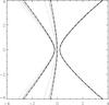 |
Fig. 4 Position of both shocks and the contact discontinuity for ηrel = 1, βp = 0.99 for increasing resolution lmax = 10 (thin dotted line), 11 (thick dotted line), 12 (dashed line), 13 (solid line). The last two resolutions give the same result. |
3.3. Geometry of the colliding wind region
Figure 5 shows the density map and the Lorentz factor map for simulations with ηrel = 0.1, 1, 10, and βp = 0.99. We set the maximal resolution to lmax = 12 and checked that, for ηrel = 0.1 and 10, the positions of the discontinuities do not vary with higher resolution (see Sect. 3.2). The stellar wind is the dense flow on the right, the pulsar wind is located on the left. The analytic solution for the contact discontinuity is obtained by combining the relativistic definition of the momentum flux ratio ηrel (Eq. (24)) with the position of the contact discontinuity derived by Antokhin et al. (2004) for colliding stellar winds. The solution assumes a thin shell geometry where both shocks and contact discontinuity are merged in one single layer. The overall structure appears similar to what is found for non-relativistic flows (see e.g Fig. 5 in Paper I). However, relativistic effects have a non-negligible influence on the structure. For instance, the symmetry is broken between the cases ηrel = 0.1 and ηrel = 10, the latter showing a reconfinement shock while the former does not. The direction of the velocity in the winds is indicated on the map of the Lorentz factor. Along the line-of-centres, the winds collide head on, and when getting farther from the binary, the velocity is mostly parallel to the direction of the shocks. This corresponds to the shock tube test simulation (Sect. B.1), which required very high resolution because of the high velocity perpendicular to the shock normal (v⊥ = 0.99). The importance of the velocity transverse to the shock normal is the reason high resolution is necessary in simulations with increasing Lorentz factors in the pulsar wind.
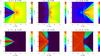 |
Fig. 5 Density (upper row) and Lorentz factor (lower row) maps for simulations with ηrel = 0.1, 1, 10 (from left to right) and βp = 0.99. The pulsar is located at x = −0.5, the star at x = 0.5. The density is given in g cm-2, the arrows show the velocity field. |
To quantify the impact of relativistic effects, we carried out simulations with ηrel = 1 for increasing values of the pulsar wind velocity βp = { 0.01,0.5,0.99,0.998 }. The corresponding Lorentz factors are Γ = { 1.00005,1.15,7.08, 15.8 }. Figure 6 shows the positions of both shocks and the contact discontinuity in the different simulations. This plot shows that, on the line-of-centres, the location of the contact discontinuity is identical in all simulations and is set by ηrel. At the edges of the box, the contact discontinuity is not exactly midplane between the winds and is closer to the pulsar. We checked that, for Mach numbers above ten, the contact discontinuity stays midplane in non-relativistic simulations with η = 1 and a different Mach number for each wind. We interpret the tilt of the CD as the impact of thermal pressure in the winds. For a given momentum flux ratio, when the pulsar wind speed is increased, its pressure is decreased, because we keep a fixed Mach number, while the stellar wind is unchanged. Thus, the higher the Lorentz factor of the pulsar wind, the more the thermal pressure from the stellar wind dominates the pulsar wind pressure. The tilt of the CD is related to our definition of the pressure in the pulsar wind, which decreases with the Lorentz factor. When we set the pressure in the pulsar wind equal to the pressure in the stellar wind, both still being small compared to the ram pressure on the line-of-centres, we find that the CD is exactly on the axis of symmetry. We consider this case to be unrealistic because the pulsar wind pressure is expected to be negligible due to adiabatic expansion (Kirk et al. 2009). The shape of the shock in the pulsar wind changes with its Lorentz factor, especially far from the binary axis. In these zones, the velocity is mostly transverse to the shock normal. Unlike the non-relativistic case, the transverse and normal velocities are tied in the jump conditions via the Lorentz factor and this has an impact on the shock location (Taub 1948). The position of the shock in the stellar wind remains unaffected by the speed of the pulsar wind. We conclude that the shape of the interaction region is affected by relativistic effects, the reason being that the pressure and transverse speed influence the relativistic jump conditions through h and Γ. The numerical tests in Appendix B.2 highlight that very high resolution is needed to properly model the shock propagation speed, when there is a high velocity perpendicular to the shock propagation direction. Although we carefully determined an adequate resolution for our simulations, a numerical effect proper to relativistic simulations cannot be excluded.
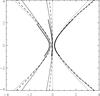 |
Fig. 6 Position of both shocks and the contact discontinuity in a simulation with ηrel = 1, in simulations with different values for the velocity of the pulsar wind : βp= 0.01 (dotted line), 0.5 (dashed line), 0.99 (solid line) and 0.998 (thick solid line). For β = 0.998 we used a smaller computational box. |
To evaluate the impact of the Lorentz factor on the hydrodynamics of the shocked region, we followed the hydrodynamical quantities along streamlines in the shocked pulsar wind. We find that, for all the values of βp, starting from the shock, the flow reaccelerates up to its initial velocity. The acceleration tends to a spherical, adiabatic expansion, with 2πsvpΓp ≡ kṀp ≃ constant (our simulations are 2D), where s is the curvilinear distance to the shock. Figure 7 shows the value of k for different speeds of the pulsar wind, for ηrel = 1. In all cases the shocked flow reaches k ≈ 3 on a scale comparable to the binary separation (increasing with βp). For ηrel = 0.1, we find the same re-acceleration, although with a higher value of k ≃ 8. The higher corresponding mass flow is due to the smaller opening angle of the shocked pulsar wind.
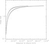 |
Fig. 7 Mass flow (Ṁp = 2πsvpΓpρp) along a streamline in the shocked pulsar wind for βp = 0.01 (dotted line), 0.5 (dashed line), and 0.99 (solid line). The mass flow is normalized to the initial mass loss rate of the pulsar, we use ηrel = 1. The simulations with βp = 0.01 and 0.5 give the same results. |
3.4. Kelvin-Helmholtz instability in gamma-ray binaries
The stellar wind has a velocity of 3000 km s-1, while the pulsar wind is almost two orders of magnitude faster. Similarly to what happens for classical flows, at the contact discontinuity between the winds, the KHI is likely to modify the structure of the flow (Blandford & Pringle 1976; Turland & Scheuer 1976). Bodo et al. (2004) find analytic solutions to the dispersion relation in RHD and show that, in the frame of the laboratory, the stability criteria are the same as in the classical case, provided one uses the relativistic definition of the Mach number (ℳrel = ℳΓ/Γcs, where Γcs is the Lorentz factor of the sound speed). In 2D simulations, we thus expect the interface between the winds to be unstable provided  .
.
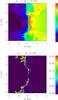 |
Fig. 8 Density (upper panel) and mixing (lower panel) maps for a simulation with ηrel = 1 and βp = 0.99. |
To verify the impact of the KHI on gamma-ray binaries, we performed a test simulation with ηrel = 1 and βp = 0.99. Radice & Rezzolla (2012) highlight the importance of an adapted Riemann solver and a low-diffusivity scheme in the study of the KHI. We used the HLLC Riemann solver to enable the development of the KHI at the contact discontinuity between the winds. This simulation displays a velocity difference (vp/vs ≃ 100). In Paper II, we found that in the classical limit, such a velocity difference leads to a significant amount of mixing between the wind and destroys the expected large scale spiral structure.
Figure 8 shows the density map and mixing between the stellar wind and the pulsar wind. The Kelvin-Helmholtz instability is clearly present in the whole colliding wind region. This is consistent with Fig.7 by Bosch-Ramon et al. (2012). In their simulation, Γp=10, ηrel = .3 and the stellar wind parameters are very close to ours, making comparison possible. Although orbital motion is included in their work, it has no impact at the location we are considering, close to the star. At a distance of about twice the binary separation, the re-acceleration of the pulsar wind means that the conditions in the shocked flow are incompatible with the analytic criterion for the developing the KHI. This suggests that the eddies present far away from the binary are due to the advection of eddies formed closer in. The eddies affect the position of the contact discontinuity but also modify the positions of both shocks. We find important differences in the position of the shock in the pulsar wind between two successive outputs, which indicates variation on a timescale of at most ten days. The KHI induces some mixing between the winds, although it occurs mostly in low-density parts of the shocked region.
The overall structure is similar to what we found for colliding non-relativistic stellar winds, for η = 1,v1/v2 = 20 (see Fig. 5 in Paper I) and in a test simulation with η = 1,v1/v2 = 100 (with the same resolution as in the relativistic simulation). Still in the classical limit, the mixed region covers a larger domain, with parts of the faster wind crossing the contact discontinuity and being totally embedded in the slower, denser wind. The mixed region seems smoother and less broken up in the classical limit. Comparison between both simulations is not straightforward because the density jump between both winds is about two orders of magnitude higher in the relativistic simulation, which probably decreases the growth of the intsability.
Bosch-Ramon et al. (2012) have simulated the large scale structure of gamma-ray binaries including orbital motion in 2D. Their simulations of the short-period binary LS 5039 show strong instabilities far from the binary, which they partly attribute to the accelerated transonic flow being deflected by the slower stellar wind and producing an unstable shocked structure. Whether this effect holds for higher values of the Lorentz factor and systems with longer orbital periods (such as PSR B1259-63) is worth investigating further.
4. Discussion: scaling to realistic pulsar winds
The simulations we performed have highlighted some similarities and differences between the interaction of classical stellar winds and the interaction between a stellar wind and a relativistic pulsar wind. This raises two questions:
-
To what extent can simulations in the classical limit provideinformation on the structure of gamma-ray binaries?
-
How can the results of relativistic simulations be extrapolated to more realistic values for the pulsar wind velocity (Γp ≃ 104 − 6) ?
Pulsar winds are characterized by the spindown power Ėp carried by the wind, which can be estimated from timing of the pulse period. The corresponding momentum flux ratio can be expressed as a function of Ėp by noticing that  and vp ≈ c so
 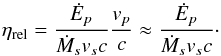 (26)Using this ηrel provides a good indication for the position of the contact discontinuity between the winds and may be used to rescale simulations of non-relativistic colliding stellar winds. Nonetheless, we found that the pulsar wind is more collimated than expected when we carried out relativistic simulations where the pulsar wind pressure Pp is lower than the stellar wind pressure Ps, even though both pressures are negligible compared to the ram pressure term ρΓ2v2 on the line-of-centers (Eq. (22)). The difference probably occurs because the relativistic jump conditions are coupled by Γ and h, with the strongest impact in the shock wings where the speed is mostly transverse to the shock. In contrast, Bogovalov et al. (2008) find that the location of the contact discontinuity in their RHD simulations is identical to the classical case, with η calculated using Eq. (26). We suspect that they obtain this result because they set the pressure exactly to zero in both winds. We recover the classical result if we set the pressure to the same value in both winds.
Since a realistic pulsar wind has Pp ≈ 0 ≪ Ps ≠ 0, our results suggest that pulsar winds are more collimated than assumed by extrapolating from classical results. This may have a significant impact on the interpretation of the radio VLBI maps of gamma-ray binaries, where the collimated radio emission has been modelled as synchrotron emission from the shocked pulsar wind (Dhawan et al. 2006; Moldón et al. 2011a,b, 2012). In particular, Romero et al. (2007) notes that the collimation angles in the binary LSI +61°303 were too narrow compared to the ones expected in the classical limit. Simulations at higher values of the Lorentz factor are highly desirable to confirm this and fully explore the impact of the wind pressure on shock location.
To easy comparison with colliding stellar winds, we assumed a constant adiabatic index γ = 5/3 in our simulation. While this is realistic for the stellar wind and (cold) unshocked pulsar wind, the adiabatic index of the (warm) shocked pulsar wind is probably close to four thirds. Performing a test simulation with ηrel = 1, βp = .99, and γ = 4/3 in both winds, we find that the shocked region in the pulsar wind is about 60% denser than when γ = 5/3, and slightly narrower. These results are consistent with what we observed in Fig. 2. However, the exact impact on gamma-ray binaries is not straightforward, since the adiabatic index transitions from the non-relativistic to the ultrarelativistic limit. As can be seen in shock tests in Figs. 5–7 of Ryu et al. (2006), when a relativistic equation of state is used, although the density jump is confined by the two limiting cases, the exact hydrodynamical structure is more complex than a simple intermediate between the cases γ = 4/3 and 5/3.
Simulations with moderate values for the Lorentz factors provide information on the density and velocity structure of the shocked flow that is useful for calculating emission properties of the system. We found that the shocked pulsar wind reaccelerates to its initial Lorentz factor and reaches an asymptotic regime with 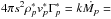 constant (or equivalently for our cylindrical 2D geometry
 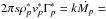 constant, with stars for quantities in the shocked region). We find that k is of order unity and is related to the opening angle of the shocked region and seems independent of the Lorentz factor of the pre-shock flow. Since the shocked wind accelerates up to its initial (i.e. pre-shock) velocity on a distance of a few times the binary separation, we have
  , and this implies that, asymptotically, the density in the shocked wind is given by
 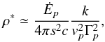 (27)where we have used
  .
.
We have verified this relation by measuring the density ratio in the shocked pulsar wind for the simulation with βp = 0.5 and βp = 0.99. Following Eq. (27), we expect ρ0.5/ρ0.99 ≃ 150. At the edge of our simulation domain, where s ≃ 4a, we find that ρ0.5/ρ0.99 varies between 140 and 155. This method assumes the flow has reached its terminal velocity. It can be used to estimate the density in the shocked pulsar wind for any value of its Lorentz factor, even using simulations in the non-relativistic limit. However, it is unable to precisely indicate the properties of the flow close to the binary. Similar caveats were found by Komissarov & Falle (1996), who proposed scaling relations to model non-relativistic equivalents of relativistic jets using the mass, energy or momentum flux. Equating the momentum flux leads to the most satisfactory results on the global morphology of the jet but still underestimates the size of the region with the highest Lorentz factors (Rosen et al. 1999).
The above ideal picture for the shocked flow is likely to be affected by the development of instabilities. Analytic work and simulations indicate that highly relativistic flows are less subject to the Kelvin-Helmholtz instability. Martí et al. (1997); Perucho et al. (2004b,a) indicate that cold jets with high Lorentz factors are more stable than slow, warm jets. In fast flows the timescale for the growth of the KHI is too long with respect to the dynamical time, while in cold flows the sound speed is low and perturbations propagate too slowly. In those particular systems, the specific axisymmetric geometry plays a role in the development of particular modes of the instability and makes it hard to directly remap the results to gamma-ray binaries.
Our simulations show that the KHI affects the positions of the shocks and induces some mixing between the winds. The most favourable conditions for developing the KHI occur close to the binary, where the shocked pulsar wind is subsonic and only mildly relativistic. Since the downstream velocity cannot be higher than c/3 for ultrarelativistic flows, the conditions for the developing the KHI are likely to be met in real systems (having Γp ≃ 104 − 6), at least close to the binary. The presence of the KHI further may be due to advection alone. Simulations at higher Lorentz factors are necessary to determine whether the unstable region is large enough to enable important growth before the advection phase begins. This is a key aspect since strong instabilities will induce mixing between the stellar and pulsar wind, which is likely to thermalize the high-energy particles of the pulsar wind and thus decrease their high-energy emission.
5. Conclusion and perspectives
We have developed a special relativistic extension to the adaptive-mesh refinement code RAMSES. We implemented two different second-order schemes and Riemann solvers. So far, only the so-called classical equation of state has been implemented, but the code was written in order to make the implementation of more complex equations of state straightforward. The code is fully three-dimensional and allows using adaptive mesh refinement. To model high-velocity flows, we included the possibility of refining cells according to the gradient of the Lorentz factor. Our code passes all of the common numerical tests in 1D, 2D, and 3D, including the most stringent tests with high Lorentz factors and velocities perpendicular to the flow.
Using this new relativistic code, we performed a 2D study of the geometry of the gamma-ray binaries, with Lorentz factors up to 16. The relativistic nature of the pulsar wind changes the momentum balance between the winds. The position of the shock in the pulsar wind is affected by the impact of the pre-shock wind pressure and transverse velocity on the shock. We found this makes the shocked pulsar wind more collimated than expected using classical hydrodynamics. This relativistic effect is strongest where the flow is essentially along the shock, far from the stagnation point. Comparing simulations with increasing values for the Lorentz factor of the pulsar wind, we find that the shocked pulsar wind re-accelerates up to its initial velocity on a scale of a few times the binary separation. We determine a prescription for the density in the shocked pulsar wind, which can be used for any value of the Lorentz factor. We find that the Kelvin-Helmholtz instability develops at the contact discontinuity affects the structure of the shocked region. Still, the exact understanding of the instability at realistic values of the pulsar wind Lorentz factor, in the particular geometry of gamma-ray binaries still needs to be confirmed. Our simulations provide clues do understanding the physics of gamma-ray binaries. However, detailed comparison with observations requires including more complex physical effects.
This code will be part of the next public release of RAMSES. It is well suited to study many astrophysical flows including gamma-ray bursts, pulsar wind nebulae, and jets in galactic binaries or active galactic nuclei. As an example, the Lorentz factor inferred from the prompt emission of gamma-ray bursts is of order 100, while the afterglow emission is related to a bulk motion of Γ ≃ 10 (see Gehrels et al. 2009, for a review) for a review). Following the fireball model, such systems display a very wide range of lengthscales, from the progenitor to decelaration radius of the forward shock, including the reverse shock and the structure of the internal shocks. Although the fully consistent study of such systems is still out of reach, the possibility for adaptive mesh refinement makes RAMSES a useful tool to model gamma-ray bursts. Our work on gamma-ray binaries can be easily adapted to simulating pulsar winds interacting with the interstellar medium or a supernova remnant. In such cases, the shock occurs further from the pulsar than in gamma-ray binaries, and the typical size of the interaction region is a few pc. This increase in length scales makes the use of AMR even more fundamental when modelling the structure and instabilities in pulsar wind nebulae.
Online material
Appendix A: Numerical scheme for RAMSES-RHD
This Appendix provides the Jacobian matrices and their eigenstructure for reconstructing the primitive variables in the 3D-RHD case. It also explains the recovery of the primitive variables.
Appendix A.1: Recovering the primitive variables
To determine the primitive variables (ρ,vj,P)T, we simplify the method by Mignone & McKinney (2007), initially developed for relativistic magnetohydrodynamics. One rewrites the total energy  (A.1)and solves an equation on W′ = W − D = ρhΓ2 − ρΓ.
To avoid numerical problems in the non-relativistic or ultrarelativistic limits, one introduces  (A.2)such that the Lorentz factor is given by
  (A.3)This gives
 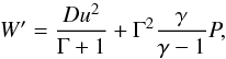 (A.4)which can be used to replace P in Eq. (A.1). Once W′ is found using, say, a Newton-Raphson method, one recovers the Lorentz factor using Eqs. (A.2) and (A.3), then the density ρ = D/Γ and finally pressure using Eq. (A.4). We determine W′ with a precision of 10-10.
The method can be easily adapted to different equations of state, by simply changing Eq. (A.4). It is well suited to codes with AMR since an initial guess of the value of W0, which guarantees the positivity of pressure, can be found analytically (Mignone & McKinney 2007). This avoids storing values of W′ between time steps, which can be cumbersome on a changing grid. One can determine W0, which then gives  , rewriting the pressure as
  (A.5)since M2 ≡ W2v2. Pressure is thus guaranteed to be positive when
  (A.6)This happens for any W > W+, with W+ the largest of the two roots of the quadratic equation Eq. (A.6). As v < 1, solving Eq. (A.6) for v = 1, implies that the corresponding root W+ ,1 > W+ ,v, which guarantees positive pressure. One thus uses W+ ,1 as the initial guess to start the Newton-Raphson scheme.
Provided the vector of conservative variables is physical, this method converges to a physical primitive state. The positivity of the density can be verified by D > 0. Subluminal velocity is guaranteed by E2 > M2 + D2. Indeed, using Eq. (6) one has  (A.7)This necessarily implies positive pressure and v < 1. Whenever a non-physical conserved state occurs, we floor the density to ρ = 10-10 and the pressure to P = 10-20. This occurs roughly once every 106 updates in our gamma-ray binary simulations. It occurs in the unshocked pulsar wind, where the density and pressure are lowest and the Lorentz factor the highest. It mostly occurs along the line of centers of the binary, since the Cartesian grid is unable to perfectly model the spherical symmetry of the wind. The number of failures strongly reduces with resolution. Beckwith & Stone (2011) note a few failures when pressure is very low and suggest using the entropy instead of the energy as conserved variable in those cases. Reconstruction by using the neighbouring cells is very cumbersome owing to the AMR structure in RAMSES, so we have not considered this option.
Appendix A.2: Computing the time step
The time step is determined by the Courant condition for unsplit schemes  (A.8)where CCFL is the Courant number and λk is the propagation speed along direction k determined by
 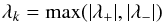 (A.9)with
 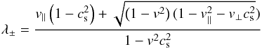 (A.10)where v∥ and v⊥ are the velocity parallel and perpendicular to the direction k. All the simulations in this paper were performed using CCFL = .8.
Our determination of the time step is more restrictive than the more commonly used (see e.g. Mignone et al. 2012) 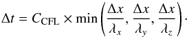 (A.11)Using the above expression for the time step, we find that the simulation of the 3D jet (Appendix B.3) shows no failure for CCFL ≤ .5, which is comparable to other codes (Zhang & MacFadyen 2006).
Appendix A.3: Jacobian matrices of the 3D-RHD equations
This section will only be available online. One has 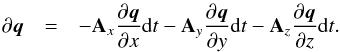 (A.12)Following Font et al. (1994) for a 1D flow with transverse velocity and the general definition of the enthalpy
 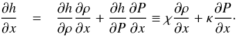 (A.13)With these definitions, the sound speed can be written as
  (A.14)For the classical equation of state, one has
  The complete Jacobian matrix is given by
  (A.17)
 with N = ( − h + hρκ + ρχv2)Γ2.
The matrix Ay is given by 
![Mathematical equation: \appendix \setcounter{section}{1} \begin{eqnarray*} \\[-0.4cm] Nc_{25}&=&\frac{-(v_xv_y(-h+\rho\chi+h\rho \kappa))}{\rho h}\\ Nc_{31}&=&0\\ Nc_{32}&=&0\\ Nc_{33}&=&v_y\Gamma^2(\rho \chi -h +h \rho \kappa)\\ Nc_{34}&=&0\\[1mm] Nc_{35}&=&\frac{1}{\rho h \Gamma^2}\left(\rho h \Gamma^2\kappa\left(1\!-\! v_y^2\right) -h -h\Gamma^2\left(v_x^2+v_z^2\right)\!+\!\rho \chi \Gamma^2\left(v_x^2\!+\!v_z^2\right)\right)\\[1mm] Nc_{41}&=&0\\ Nc_{42}&=&0\\ Nc_{43}&=&v_z\rho\chi\\ Nc_{44}&=&v_yN\\[1mm] Nc_{45}&=&\frac{-v_xv_z(-h+\rho\chi+\rho h\kappa)}{\rho h}\\[1mm] Nc_{51}&=&0\\ Nc_{52}&=&0\\ Nc_{53}&=&-\rho^2 h\Gamma^2\chi\\ Nc_{54}&=&0\\ Nc_{55}&=&v_y\Gamma^2(\rho \chi -h +h \rho \kappa). \end{eqnarray*}](/articles/aa/full_html/2013/12/aa22266-13/aa22266-13-eq211.png) Along z one has Az given by
Along z one has Az given by ![Mathematical equation: \appendix \setcounter{section}{1} \begin{eqnarray*} Nc_{11}&=& v_zN\\ Nc_{12}&=& 0\\ Nc_{13}&=& 0\\ Nc_{14}&=& h\rho\Gamma^2(\rho\kappa-1)\\[1mm] Nc_{15}&=&v_z\left(-\rho \Gamma^2\kappa+\rho v^2\Gamma^2\kappa+1\right)\\[1mm] Nc_{21}&=&0\\ Nc_{22}&=&v_zN\\ Nc_{23}&=&0\\ Nc_{24}&=&v_z\rho \chi\\[1mm] Nc_{25}&=&\frac{-v_xv_z(-h+\rho\chi+\rho h\kappa)}{\rho h}\\[1mm] Nc_{31}&=&0\\ Nc_{32}&=&0\\ Nc_{33}&=&v_zN\\ Nc_{34}&=&v_y\rho\chi\\[1mm] Nc_{35}&=&\frac{-v_yv_z(-h+\rho\chi+\rho h\kappa)}{\rho h}\\[1mm] Nc_{41}&=&0\\ Nc_{42}&=&0\\ Nc_{43}&=&0\\ Nc_{44}&=&v_z\Gamma^2(\rho \chi -h +h \rho \kappa)\\[1mm] Nc_{45}&=&\frac{1}{\rho h \Gamma^2}\left(\rho h \Gamma^2\kappa\left(1\! -\! v_z^2\right) -h -h\Gamma^2\left(v_x^2\! +\! v_y^2\right)\! +\! \rho \chi \Gamma^2\left(v_x^2+v_y^2\right)\right)\\[1mm] Nc_{51}&=&0\\ Nc_{52}&=&0\\ Nc_{53}&=&0\\ Nc_{54}&=&-\rho^2 h \Gamma^2\chi\\ Nc_{55}&=&v_z\Gamma^2(\rho \chi -h +h \rho \kappa). \end{eqnarray*}](/articles/aa/full_html/2013/12/aa22266-13/aa22266-13-eq213.png)
Appendix A.4: Eigenstructure
 |
Fig. B.1 Density, AMR levels (red dashed line), parallel and transverse velocity and pressure in the frame of the laboratory for the shock test with Γmax = 120. Left panels: uniform grid nx = 512; middle panels: uniform grid nx = 217 = 131072; right panels: nx = 64, lmax = 17. The black solid line represents the MUSCL method, while the black dashed line represents the PLM method. At high resolution, they give the same result, which is very close to the analytic solution. |
The eigenvalues of Ax are (see e.g. Falle & Komissarov 1996)  with
with  (A.23)The left eigenvectors are given by
 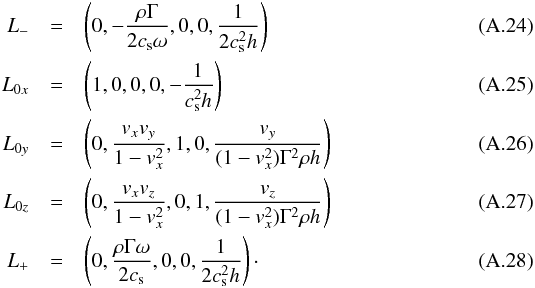 The right eigenvectors are given by
 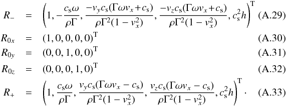 Similarly for Ay one has
 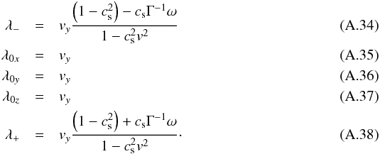 with
with  (A.39)The left eigenvectors are given by
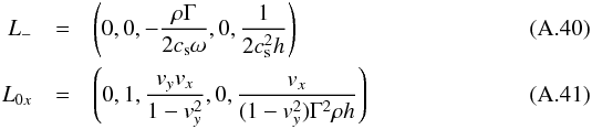
![Mathematical equation: \appendix \setcounter{section}{1} \begin{eqnarray} \nonumber\\[-0.5cm] L_{0y}&=& \left(1,0,0,0,-\frac{1}{c_{\rm s}^2h}\right)\\ L_{0z}&=& \left(0, 0, \frac{v_yv_z}{1-v_y^2},1,\frac{v_z}{\left(1-v_y^2\right)\Gamma^2\rho h}\right)\\ L_+&=&\left(0,0,\frac{\rho \Gamma} { 2 c_{\rm s} \omega}, 0, \frac{1}{2 c_{\rm s}^2 h}\right)\cdot \end{eqnarray}](/articles/aa/full_html/2013/12/aa22266-13/aa22266-13-eq226.png) The right eigenvectors are given by
The right eigenvectors are given by 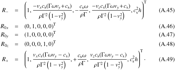 For Az one has
 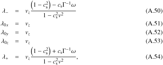 with
with  (A.55)The left eigenvectors are given by
 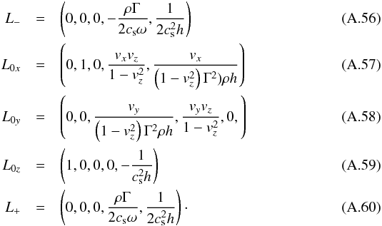 The right eigenvectors are given by
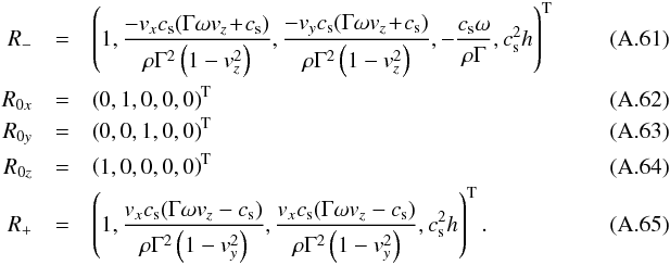
Appendix B: Numerical tests
In this section, we present a set of numerical tests that validate our new relativistic code. Unless stated differently, all the simulations were performed with Courant number CCFL = 0.8, the minmod slope limiter in the MUSCL scheme and for the AMR prolongations, and the HLLC Riemann solver. The adiabatic index is set to 5/3. Refinement is based on density and velocity gradients.
Appendix B.1: 1D Sod test
One initially starts with two different media separated by an interface located at x = 0.5. When the simulation begins, the interface is removed and the flow evolves freely following a self-similar structure. The flow decays into three waves, usually a rarefaction, a contact discontinuity, and a shock. These tests are very common because easy to implement and comparisons with analytic solutions are possible (see Martí & Müller 1994, for pioneering work; and Rezolla et al. 2003, for an elegant version including transverse velocities).
We reproduce the test of Sect. 2.3, with a maximal Lorentz factor of 120. Contrary to the Newtonian case, transverse velocities do impact the shock structure in RHD and reduce the shock velocity. Several groups have shown that tests with high transverse velocities are very stringent and only show satisfactory results at very high resolution (Mignone & Bodo 2005; Zhang & MacFadyen 2006).
Figure B.1 gives the density, parallel, and transverse velocity and pressure at tend = 1.8 for tests with different resolutions. The thick black line represents the simulation using the MUSCL scheme with the minmod limiter while the dashed line represents the simulation following the PLM method with the moncen limiter. Both methods lead to similar results. The AMR levels are superposed on the density plots. Refinement is based on the gradients of both the Lorentz factor and pressure. The first simulation has a uniform resolution of 512 cells, which is close to the resolution used by Mignone et al. (2005). Our simulation is similar to theirs, with the shock running ahead of its theoretical position and some inaccuracy in the orientation of the velocity vector. These discrepancies reduce with increasing resolution. In the second simulation, the resolution is also uniform but set to 217 = 131 072 cells. This is the same resolution as Ryu et al. (2006), and we obtain very good agreement with their results and the analytic solution. At high resolution, there is no clear difference between the PLM and MUSCL method. However, such high resolution is prohibitive in multidimensional simulations. The last panel shows a simulation with AMR, the coarse level is set by nx = 64, while the highest level lmax = 17. The result is in very good agreement with the expected solution. The density difference between our results and the analytic solution is lower than one percent, even at the discontinuities. At the end of the test, the gain of computing time is about a factor 200 compared to the uniform grid. A simulation with the same computing time, but on a uniform grid would have a resolution of slightly more than 4096 cells. A test simulation with a uniform resolution nx = 4096 showed a 40% discrepancy in the density at the beginning of the shocked region, with respect to the analytic solution. AMR proves to be very helpful tool in the modelling of highly relativistic flows.
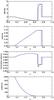 |
Fig. B.2 Inclined shock test: density, velocity, pressure and Lorentz factor along the shock normal. The thick solid lines give the 2D results, the dot-dashed lines the 1D results from a simulation with the same resolution, and the blue lines give the analytic solution. The resolution is lower than for the 1D test in Sect. B.1. |
Appendix B.2: 2D Inclined shock tube
Two-dimensional tests are important to verify the accuracy of the coupling between the different components of the four-vectors. We performed the above Sod tests by inclining the interface between the two media by θ = 21.7° with respect to a vertical line. The value of θ is chosen arbitrarily to avoid any peculiar alignement with respect to the numerical grid, as could occur for θ = 45° (Radice & Rezzolla 2012). Since the initial separation between both sides is inclined, for a given y, the initial conditions are shifted by a few cells with repect to the row of cells just below. The boundary conditions along the y axis follow the same shift. At the bottom boundary one has 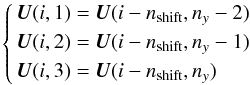 (B.1)for all the cells with i − nshift = i − (ny × tanθ) > 0. The boundary conditions are periodic along the x axis. The simulations took 2200 CPU hours.
The simulations should give a comparable result to 1D simulations with the same resolution. Figure B.2 shows the different variables in the direction normal to the shock for the second test using a 12 800 × 6400 uniform resolution. The given values were obtained by performing a bilinear interpolation of the 2D simulation. We overplot the analytic solution and the result from a 1D simulation with the same resolution along the interface between the flows (ny/cosθ = 6400 cells). The 2D simulation differs somewhat from its equivalent 1D simulation. This suggests that direct comparison between unidimensional and multidimensional simulations is not possible and that, for high Lorentz factors, multidimensional simulations need a higher resolution to be numerically accurate.
In both the 1D and the 2D simulations, the position of the shock is ahead of its theoretical position. The 1D and 2D tests have shown that this effect weakens at higher resolution.
Appendix B.3: 3D jet
Relativistic jets have become a widespread way to test multidimensional RHD codes. Their complex dynamics show the impact of transverse velocities and display the development of instabilities. In this case, no analytic solution exists, and validation is done by comparison with former results. We follow the setup by Del Zanna & Bucciantini (2002)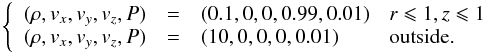 The length scale is given by the initial radius of the jet r0 = 1, the size of the box is 20r0, with lmin = 6 and lmax = 9. This gives an equivalent resolution of 25 cells per radius, while the original test was performed with a resolution of 20 cells per radius. We perform a 3D simulation, while most jets are simulated using axisymmetric 2D simulations (Lucas-Serrano et al. 2004). Except at the injection of the jet, we use outflow boundary conditions. The maximum Lorentz factor is 7.1. The evolution of the density profile is given in Fig. B.3. One can see the typical features of relativistic jets: the bow shock with the external medium, the cocoon of shocked medium, the relativistic beam, and the Mach disk. The Kelvin-Helmholtz instability develops at the interface between the shocked external medium and the shocked material from the jet. The overall shape is similar to the simulation by Del Zanna & Bucciantini (2002) although the simulation with RAMSES-RHD presents a small extension at the head of the jet. This is due to the carbuncle instability (Peery & Imlay 1988), which arises when cylindrical or spherical phenomena are simulated on a Cartesian grid. Performed on 16 processors, this simulation took 320 mono-CPU hours. The same simulation on a 5123 fixed grid took about 500 h. Owing to the complex structure inside the jet, AMR is not very efficient in this type of simulation (Zhang & MacFadyen 2006).
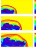 |
Fig. B.3 Simulation of the propagation of a 3D relativistic jet (Γmax = 7.1). From top to bottom: density at t = 20,30,40 in a 3D jet starting from the left boundary of the domain. |
Acknowledgments
This work was supported by the European Community via contract ERC-StG-200911. Calculations have been performed at the CEA on the DAPHPC cluster and using HPC resources from GENCI-[CINES] (Grants 2012046391-2013046391). The authors thank B. Giacomazzo for sharing his code for determining analytic solutions of relativistic shock tubes.
References
- Aharonian, F., Akhperjanian, A. G., Aye, K.-M., et al. 2005a, Science, 309, 746 [NASA ADS] [CrossRef] [PubMed] [Google Scholar]
- Aharonian, F., Akhperjanian, A. G., Aye, K.-M., et al. 2005b, A&A, 442, 1 [Google Scholar]
- Albert, J., Aliu, E., Anderhub, H., et al. 2006, Science, 312, 1771 [NASA ADS] [CrossRef] [PubMed] [Google Scholar]
- Aloy, M. A., Ibáñez, J., Martí, J. M., & Müller, E. 1999, ApJS, 122, 151 [NASA ADS] [CrossRef] [Google Scholar]
- Antokhin, I. I., Owocki, S. P., & Brown, J. C. 2004, ApJ, 611, 434 [NASA ADS] [CrossRef] [Google Scholar]
- Beckwith, K., & Stone, J. M. 2011, ApJS, 193, 6 [NASA ADS] [CrossRef] [Google Scholar]
- Blandford, R. D., & Pringle, J. E. 1976, MNRAS, 176, 443 [NASA ADS] [CrossRef] [Google Scholar]
- Bodo, G., Mignone, A., & Rosner, R. 2004, Phys. Rev. E, 70, 036304 [NASA ADS] [CrossRef] [Google Scholar]
- Bogovalov, S. V., Khangulyan, D. V., Koldoba, A. V., Ustyugova, G. V., & Aharonian, F. A. 2008, MNRAS, 387, 63 [NASA ADS] [CrossRef] [Google Scholar]
- Bogovalov, S. V., Khangulyan, D., Koldoba, A. V., Ustyugova, G. V., & Aharonian, F. A. 2012, MNRAS, 419, 3426 [NASA ADS] [CrossRef] [Google Scholar]
- Bongiorno, S. D., Falcone, A. D., Stroh, M., et al. 2011, ApJ, 737, L11 [NASA ADS] [CrossRef] [Google Scholar]
- Bosch-Ramon, V., & Barkov, M. V. 2011, A&A, 535, A20 [NASA ADS] [CrossRef] [EDP Sciences] [Google Scholar]
- Bosch-Ramon, V., Barkov, M. V., Khangulyan, D., & Perucho, M. 2012, A&A, 544, A59 [NASA ADS] [CrossRef] [EDP Sciences] [Google Scholar]
- Bucciantini, N. 2002, A&A, 387, 1066 [NASA ADS] [CrossRef] [EDP Sciences] [Google Scholar]
- Bucciantini, N., Blondin, J. M., Del Zanna, L., & Amato, E. 2003, A&A, 405, 617 [NASA ADS] [CrossRef] [EDP Sciences] [Google Scholar]
- Bucciantini, N., Amato, E., & Del Zanna, L. 2005, A&A, 434, 189 [NASA ADS] [CrossRef] [EDP Sciences] [Google Scholar]
- Collela, P. 1990, J. Comput. Phys., 87, 171 [NASA ADS] [CrossRef] [Google Scholar]
- Del Zanna, L., & Bucciantini, N. 2002, A&A, 390, 1177 [NASA ADS] [CrossRef] [EDP Sciences] [Google Scholar]
- Del Zanna, L., Volpi, D., Amato, E., & Bucciantini, N. 2006, A&A, 453, 621 [NASA ADS] [CrossRef] [EDP Sciences] [Google Scholar]
- Dhawan, V., Mioduszewski, A., & Rupen, M. 2006, in Proc. VI Microquasar workshop: microquasars and beyond, 52 [Google Scholar]
- Dubus, G. 2006, A&A, 456, 801 [NASA ADS] [CrossRef] [EDP Sciences] [Google Scholar]
- Duffell, P. C., & MacFadyen, A. I. 2011, ApJS, 197, 15 [NASA ADS] [CrossRef] [Google Scholar]
- Falle, S. A. E. G., & Komissarov, S. S. 1996, MNRAS, 278, 586 [NASA ADS] [CrossRef] [Google Scholar]
- Fermi LAT Collaboration, Ackermann, M., Ajello, M., et al. 2012, Science, 335, 189 [NASA ADS] [CrossRef] [Google Scholar]
- Font, J. A., Ibáñez, J. M., Marquina, A., & Martí, J. M. 1994, A&A, 282, 304 [NASA ADS] [Google Scholar]
- Fromang, S., Hennebelle, P., & Teyssier, R. 2006, A&A, 457, 371 [NASA ADS] [CrossRef] [EDP Sciences] [Google Scholar]
- Gehrels, N., Ramirez-Ruiz, E., & Fox, D. B. 2009, ARA&A, 47, 567 [NASA ADS] [CrossRef] [Google Scholar]
- Giacomazzo, B., & Rezzolla, L. 2006, J. Fluid Mech., 562, 223 [Google Scholar]
- Hughes, P. A., Miller, M. A., & Duncan, G. C. 2002, ApJ, 572, 713 [NASA ADS] [CrossRef] [Google Scholar]
- Johnston, S., Manchester, R. N., Lyne, A. G., et al. 1992, ApJ, 387, L37 [Google Scholar]
- Keppens, R., Meliani, Z., van Marle, A., et al. 2012, J. Comput. Phys., 231, 718 [Google Scholar]
- Kirk, J. G., Lyubarsky, Y., & Petri, J. 2009, in Astrophys. Space Sci. Lib. 357, ed. W. Becker, 421 [Google Scholar]
- Komissarov, S. S., & Falle, S. A. E. G. 1996, in Energy transport in radio galaxies and quasars, eds. P. E. Hardee, A. H. Bridle, & J. A. Zensus, ASP Conf. Ser., 100, 173 [Google Scholar]
- Komissarov, S. S., & Lyubarsky, Y. E. 2004, MNRAS, 349, 779 [NASA ADS] [CrossRef] [Google Scholar]
- Kravtsov, A. V., Klypin, A. A., & Khokhlov, A. M. 1997, ApJS, 111, 73 [NASA ADS] [CrossRef] [Google Scholar]
- Lamberts, A., Fromang, S., & Dubus, G. 2011, MNRAS, 418, 2618 (Paper I) [NASA ADS] [CrossRef] [Google Scholar]
- Lamberts, A., Dubus, G., Lesur, G., & Fromang, S. 2012, A&A, 546, A60 (Paper II) [NASA ADS] [CrossRef] [EDP Sciences] [Google Scholar]
- Landau, L., & Lifshitz, D. 1959, The classical theory of fields, ed. P. Press (Butterworth-Heinemann) [Google Scholar]
- Lemaster, M. N., Stone, J. M., & Gardiner, T. A. 2007, ApJ, 662, 582 [NASA ADS] [CrossRef] [Google Scholar]
- Lucas-Serrano, A., Font, J. A., Ibáñez, J. M., & Martí, J. M. 2004, A&A, 428, 703 [NASA ADS] [CrossRef] [EDP Sciences] [Google Scholar]
- Martí, J. M., & Müller, E. 1994, J. Fluid Mech., 258, 317 [NASA ADS] [CrossRef] [Google Scholar]
- Martí, J. M., & Müller, E. 2003, Liv. Rev. Rel., 6, 7 [Google Scholar]
- Martí, J. M. A., Müller, E., Font, J. A., Ibáñez, J. M. A., & Marquina, A. 1997, ApJ, 479, 151 [NASA ADS] [CrossRef] [Google Scholar]
- Mignone, A., & Bodo, G. 2005, MNRAS, 364, 126 [NASA ADS] [CrossRef] [Google Scholar]
- Mignone, A., & McKinney, J. C. 2007, MNRAS, 378, 1118 [Google Scholar]
- Mignone, A., Plewa, T., & Bodo, G. 2005, ApJS, 160, 199 [NASA ADS] [CrossRef] [Google Scholar]
- Mignone, A., Zanni, C., Tzeferacos, P., et al. 2012, ApJS, 198, 7 [Google Scholar]
- Moldón, J., Johnston, S., Ribó, M., Paredes, J. M., & Deller, A. T. 2011a, ApJ, 732, L10 [NASA ADS] [CrossRef] [Google Scholar]
- Moldón, J., Ribó, M., & Paredes, J. M. 2011b, A&A, 533, L7 [NASA ADS] [CrossRef] [EDP Sciences] [Google Scholar]
- Moldón, J., Ribó, M., & Paredes, J. M. 2012, A&A, 548, A103 [NASA ADS] [CrossRef] [EDP Sciences] [Google Scholar]
- Noble, S. C., Gammie, C. F., McKinney, J. C., & Del Zanna, L. 2006, ApJ, 641, 626 [NASA ADS] [CrossRef] [Google Scholar]
- Parkin, E. R., Pittard, J. M., Corcoran, M. F., & Hamaguchi, K. 2011, ApJ, 726, 105 [NASA ADS] [CrossRef] [Google Scholar]
- Peery, K., & Imlay, S. 1988, in Proc. 24th Joint propulsion conf., AIAA, 88, 2904 [Google Scholar]
- Perucho, M., Hanasz, M., Martí, J. M., & Sol, H. 2004a, A&A, 427, 415 [NASA ADS] [CrossRef] [EDP Sciences] [Google Scholar]
- Perucho, M., Martí, J. M., & Hanasz, M. 2004b, A&A, 427, 431 [NASA ADS] [CrossRef] [EDP Sciences] [Google Scholar]
- Pittard, J. M. 2009, MNRAS, 396, 1743 [NASA ADS] [CrossRef] [Google Scholar]
- Pons, J. A., Martí, J., & Müller, E. 2000, J. Fluid Mech., 422, 125 [NASA ADS] [CrossRef] [Google Scholar]
- Puls, J., Vink, J. S., & Najarro, F. 2008, A&ARv, 16, 209 [NASA ADS] [CrossRef] [EDP Sciences] [Google Scholar]
- Radice, D., & Rezzolla, L. 2012, A&A, 547, A26 [NASA ADS] [CrossRef] [EDP Sciences] [Google Scholar]
- Rezolla, L., Zanotti, O., & Pons, J. 2003, J. Fluid Mech., 479, 199 [NASA ADS] [CrossRef] [Google Scholar]
- Roe, P. L. 1986, Ann. Rev. Fluid Mech., 18, 337 [NASA ADS] [CrossRef] [Google Scholar]
- Romero, G. E., Okazaki, A. T., Orellana, M., & Owocki, S. P. 2007, A&A, 474, 15 [NASA ADS] [CrossRef] [EDP Sciences] [Google Scholar]
- Rosen, A., Hughes, P. A., Duncan, G. C., & Hardee, P. E. 1999, ApJ, 516, 729 [NASA ADS] [CrossRef] [Google Scholar]
- Ryu, D., Chattopadhyay, I., & Choi, E. 2006, ApJS, 166, 410 [NASA ADS] [CrossRef] [Google Scholar]
- Schneider, V., Katscher, U., Rischke, D., et al. 1993, J. Comput. Phys., 105, 92 [NASA ADS] [CrossRef] [MathSciNet] [Google Scholar]
- Stevens, I. R., Blondin, J. M., & Pollock, A. M. T. 1992, ApJ, 386, 265 [NASA ADS] [CrossRef] [Google Scholar]
- Synge, J. 1957, The relativistic gas (North Holland Pub. Co.) [Google Scholar]
- Taub, A. H. 1948, Phys. Rev., 74, 328 [NASA ADS] [CrossRef] [Google Scholar]
- Tavani, M., Arons, J., & Kaspi, V. M. 1994, ApJ, 433, L37 [NASA ADS] [CrossRef] [Google Scholar]
- Teyssier, R. 2002, A&A, 385, 337 [NASA ADS] [CrossRef] [EDP Sciences] [Google Scholar]
- Turland, B. D., & Scheuer, P. A. G. 1976, MNRAS, 176, 421 [NASA ADS] [Google Scholar]
- van der Swaluw, E., Achterberg, A., Gallant, Y. A., Downes, T. P., & Keppens, R. 2003, A&A, 397, 913 [NASA ADS] [CrossRef] [EDP Sciences] [Google Scholar]
- van Leer, B. 1977, J. Comput. Phys., 23, 263 [NASA ADS] [CrossRef] [Google Scholar]
- van Leer, B. 1979, J. Comput. Phys., 32, 101 [Google Scholar]
- Vigelius, M., Melatos, A., Chatterjee, S., Gaensler, B. M., & Ghavamian, P. 2007, MNRAS, 374, 793 [NASA ADS] [CrossRef] [Google Scholar]
- Vishniac, E. T. 1994, ApJ, 428, 186 [NASA ADS] [CrossRef] [Google Scholar]
- Volpi, D., Del Zanna, L., Amato, E., & Bucciantini, N. 2008, A&A, 485, 337 [NASA ADS] [CrossRef] [EDP Sciences] [Google Scholar]
- Wang, P., Abel, T., & Zhang, W. 2008, ApJS, 176, 467 [NASA ADS] [CrossRef] [Google Scholar]
- Zhang, W., & MacFadyen, A. I. 2006, ApJS, 164, 255 [NASA ADS] [CrossRef] [Google Scholar]
All Figures
|
Fig. 1 Density, velocity, and pressure in the laboratory frame at t = 0.45. The thin solid line shows the PLM method, the dashed line the MUSCL metod, which gives very similar results. The analytic solution (Giacomazzo & Rezzolla 2006) is given in blue. The resolution is nx = 256. |
| In the text | |
|
Fig. 2 Density, velocity, and pressure in the laboratory frame at t = 0.45 for tests with different adiabatic indices. The black solid line shows γ = 5/3, the dashed green line shows γ = 4/3, the resolution is nx = 256. |
| In the text | |
|
Fig. 3 Density, parallel velocity, transverse velocity, and pressure in the laboratory frame for two different simulations. In both cases, the coarse grid is set by nx = 64 with 11 levels of refinement based on pressure gradients. The solid line shows a simulation where additional refinements occur based on Lorentz factor gradients. The result is superimposed to the analytic solution (Giacomazzo & Rezzolla 2006) given in blue. The red dashed line in the upper panel shows the refinement levels, based on the Lorentz factor gradients. |
| In the text | |
|
Fig. 4 Position of both shocks and the contact discontinuity for ηrel = 1, βp = 0.99 for increasing resolution lmax = 10 (thin dotted line), 11 (thick dotted line), 12 (dashed line), 13 (solid line). The last two resolutions give the same result. |
| In the text | |
|
Fig. 5 Density (upper row) and Lorentz factor (lower row) maps for simulations with ηrel = 0.1, 1, 10 (from left to right) and βp = 0.99. The pulsar is located at x = −0.5, the star at x = 0.5. The density is given in g cm-2, the arrows show the velocity field. |
| In the text | |
|
Fig. 6 Position of both shocks and the contact discontinuity in a simulation with ηrel = 1, in simulations with different values for the velocity of the pulsar wind : βp= 0.01 (dotted line), 0.5 (dashed line), 0.99 (solid line) and 0.998 (thick solid line). For β = 0.998 we used a smaller computational box. |
| In the text | |
|
Fig. 7 Mass flow (Ṁp = 2πsvpΓpρp) along a streamline in the shocked pulsar wind for βp = 0.01 (dotted line), 0.5 (dashed line), and 0.99 (solid line). The mass flow is normalized to the initial mass loss rate of the pulsar, we use ηrel = 1. The simulations with βp = 0.01 and 0.5 give the same results. |
| In the text | |
|
Fig. 8 Density (upper panel) and mixing (lower panel) maps for a simulation with ηrel = 1 and βp = 0.99. |
| In the text | |
|
Fig. B.1 Density, AMR levels (red dashed line), parallel and transverse velocity and pressure in the frame of the laboratory for the shock test with Γmax = 120. Left panels: uniform grid nx = 512; middle panels: uniform grid nx = 217 = 131072; right panels: nx = 64, lmax = 17. The black solid line represents the MUSCL method, while the black dashed line represents the PLM method. At high resolution, they give the same result, which is very close to the analytic solution. |
| In the text | |
|
Fig. B.2 Inclined shock test: density, velocity, pressure and Lorentz factor along the shock normal. The thick solid lines give the 2D results, the dot-dashed lines the 1D results from a simulation with the same resolution, and the blue lines give the analytic solution. The resolution is lower than for the 1D test in Sect. B.1. |
| In the text | |
|
Fig. B.3 Simulation of the propagation of a 3D relativistic jet (Γmax = 7.1). From top to bottom: density at t = 20,30,40 in a 3D jet starting from the left boundary of the domain. |
| In the text | |
Current usage metrics show cumulative count of Article Views (full-text article views including HTML views, PDF and ePub downloads, according to the available data) and Abstracts Views on Vision4Press platform.
Data correspond to usage on the plateform after 2015. The current usage metrics is available 48-96 hours after online publication and is updated daily on week days.
Initial download of the metrics may take a while.