| Issue |
A&A
Volume 558, October 2013
|
|
|---|---|---|
| Article Number | A48 | |
| Number of page(s) | 14 | |
| Section | Stellar atmospheres | |
| DOI | https://doi.org/10.1051/0004-6361/201321343 | |
| Published online | 04 October 2013 | |
Online material
Appendix A: Horizontal averages
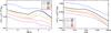 |
Fig. A.1
Average profiles of the rms fluctuations of the geometrical height on iso-τR surfaces (left) and on iso-p surfaces (right) in units of the local pressure scale heights. |
| Open with DEXTER | |
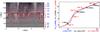 |
Fig. A.2
Illustration of the different averages. Left panel: vertical cut through a part of the G2V simulation domain. Surfaces of constant optical depth (solid, red curves) and constant pressure (dashed, blue curves) are indicated; the underlying grey-scale image illustrate the density (normalised by the horizontal mean ⟨ϱ⟩z). Right panel: run of the horizontally averaged temperature vs. averaged pressure in the G2V simulation for the different averages ⟨ · ⟩ z (dotted, black), ⟨ · ⟩ τ (red, solid), and ⟨ · ⟩ p (blue, dashed); as a reference the position of some z and τ values is marked. |
| Open with DEXTER | |
We consider temporally and horizontally averaged quantities to study the mean stratification of the six simulated stars and compare them to 1D models. Depending on the context, the sensible “horizontal” average is an average over surfaces of constant geometrical depth, (Rosseland) optical depth, or (gas) pressure, denoted by ⟨ · ⟩ z, ⟨ · ⟩ τ, or ⟨ · ⟩ p, respectively. The average ⟨ · ⟩ τ is sensible for the layers around the optical surface and in the photosphere (especially for quantities involving the emergent intensity), while the average ⟨ · ⟩ z is more relevant for the convective, deeper layers, where the stratifications are nearly adiabatic and largely independent from the radiation field. However, z is highly impractical as a coordinate scale for comparing simulations of stars of various spectral types, since the pressure scale height varies by more than a factor of ten between the six simulated stars presented in this paper (cf. Fig. 9). Therefore, we use the logarithm of the normalised pressure ⟨p⟩z/p0 as a more suitable depth coordinate (where p0 = ⟨p⟩τR = 1 is the average gas pressure at the optical surface) to illustrate depth dependences of quantities averaged on iso-z surfaces. This should not be confused with an average on surfaces of constant pressure, ⟨ · ⟩ p.
The averages ⟨ · ⟩ τ and ⟨ · ⟩ p are defined as horizontal averages of a quantity on iso-τ and iso-p surfaces, respectively. For the average ⟨ · ⟩ p, which is rarely used in this article, there is the problem that sometimes iso-p surfaces cannot be unambiguously defined since strong deviations from hydrostatic equilibrium in regions with Mach number of order unity can lead to a locally non-monotonic depth dependence of the gas pressure. Our iso-p surfaces are the deepest surfaces on which the pressure assumes the given value. This arbitrary choice does not significantly influence the results for the iso-p means in the simulations, except for the surface layers of the F3V simulation where the flows are mostly sonic and supersonic (cf. Fig. 6).
Figure A.1 shows the rms fluctuations of the geometrical depth on surfaces of constant optical depth (left panel) and pressure (right panel) as a measure of the corrugation of these surfaces. Due to this corrugation of the iso-p and iso-τR surfaces, profiles of quantities averaged in the different ways described above are not just distorted versions of each other, but can show a significantly different depth dependence of the same quantity. The differences between the three averaging methods are expected to be largest in the F- and G-type simulations, for which the corrugation of the iso-p and iso-τR surfaces is strongest.
The left panel of Fig. A.2 shows a vertical cut through some of the iso-p and iso-τR surfaces in the G2V simulation. Note that in the optically thin upper part of the simulation domain, the iso-p-surfaces follow the iso-τR surfaces. Although this is observed in all six simulations, this effect is most prominent in the G-type star (see discussion of Fig. 12 in Sect. 3.3). In the optically thick part, the temperature fluctuations determine the shape
of the iso-τR surfaces, since the opacity is highly temperature-sensitive in this regime. The iso-p surfaces, however, become almost flat planes in the deeper layers since the density contrast and deviations from hydrostatic equilibrium decrease with increasing depth.
The right panel of Fig. A.2 illustrates the different depth dependences of temperature, T, for the three different averages ⟨ · ⟩ z, ⟨ · ⟩ τ, and ⟨ · ⟩ p. As for most of the figures in this paper, the gas pressure (here without normalisation) was used as depth coordinate. For ⟨T⟩τ and ⟨T⟩z, the pressure varies along the surfaces over which the average is performed. The depth coordinates are therefore averages themselves, namely ⟨p⟩τ and ⟨p⟩z, respectively, in these cases. As expected, the differences between the differently averaged temperature are largest at the optical surface and all three averages converge at large optical depth (log τR ≳ 4). As the deviations from hydrostatic equilibrium are small in the subsurface layers, ⟨ · ⟩ p stays close to ⟨ · ⟩ z. The average ⟨ · ⟩ τ deviates more strongly near the photospheric transition since the big temperature fluctuations govern the opacity and thus lead to strongly corrugated iso-tau surfaces. In the atmosphere, the deviations between different averages of temperature become smaller with height. Especially, ⟨T⟩p ≈ ⟨T⟩τ, in these layers as expected, because the iso-τ surfaces roughly follow the iso-p surfaces.
If one aims at comparing 1D and averaged 3D results, one has to take into account that a 1D model does not have corrugated iso-τ surfaces. Profiles of quantities which change rapidly at the photospheric transition have a steep gradient in 1D models comparable to the local gradient in a 3D simulation. As the depth of the photospheric transition varies across the surface in a 3D simulation, these strong local gradients are smeared out and the similarity between 1D and averaged 3D results is obscured, if a plain horizontal average, ⟨ · ⟩ z is used. The average ⟨ · ⟩ τ is more appropriate in these cases for a comparison between 1D and averaged 3D profiles. This average however has no relevance below the photospheric transition, where ⟨ · ⟩ z is more useful. For the stellar parameters used in our simulations, the ⟨ · ⟩ p average seems a good compromise between the two other averaging methods for comparison with 1D models as it is converging towards ⟨ · ⟩ τ in the atmosphere and towards ⟨ · ⟩ z in the convection zone.
In order to obtain the temporally averaged profiles presented in this paper, first one of the horizontal averaging methods described above was applied to several snapshots with a time separation of 5–7 min, depending on the star. Then, for each quantity and at each depth point, the values of the different snapshots were averaged. The time dependence of the horizontal averages of most quantities under consideration (such as T, p, ϱ, etc.) was found to be very small, so that we found a small number of snapshots to be sufficient for a sensible temporal average. The mean profiles presented in this article are averages over six snapshots each.
© ESO, 2013
Current usage metrics show cumulative count of Article Views (full-text article views including HTML views, PDF and ePub downloads, according to the available data) and Abstracts Views on Vision4Press platform.
Data correspond to usage on the plateform after 2015. The current usage metrics is available 48-96 hours after online publication and is updated daily on week days.
Initial download of the metrics may take a while.