| Issue |
A&A
Volume 558, October 2013
|
|
|---|---|---|
| Article Number | A91 | |
| Number of page(s) | 21 | |
| Section | Planets and planetary systems | |
| DOI | https://doi.org/10.1051/0004-6361/201321132 | |
| Published online | 14 October 2013 | |
Online material
Appendix A: Departure from the Cunningham velocity
The Stokes-Cunningham velocity defined in Eq. (3)is derived under the assumption of low Reynolds number. Therefore it is not valid for turbulent flow and other expressions may be used when the Reynolds number increases. Here we derive better laws for intermediate and large Reynolds number.
Appendix A.1: Low Knudsen number
For small Reynolds number and small Knudsen number, the drag force exerted by a fluid on a sphere at rest is considered proportional to the kinetic energy of the fluid and the projected area of the sphere. The coefficient of proportionality, or drag coefficient, CD is given by: 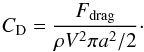 (A.1)Then, equating gravity and drag forces leads to the settling velocity of a particle in an atmosphere:
 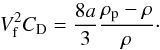 (A.2)Where ρp is the density of the particle. For small Reynolds numbers and high Knudsen number, CD = 24 is constant and the settling velocity is the Stokes velocity. When increasing the Reynolds number, the non linear terms of the Navier-Stokes equation become important and CD is no longer constant. We used tabulated values of the drag coefficient as a function of the Reynolds number given by Pruppacher & Klett (1978). We assume that CD = 24 when the Reynolds number reaches 1 to stay consistent with Stokes flow and that CD reaches its asymptotic value, CD = 0.45, when NRe ≡ 2Re = 1000 and fit the relationship:
 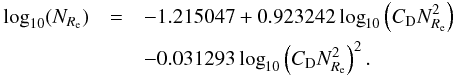 (A.3)Then we follow the same method as Ackerman & Marley (2001). Noting that:
 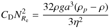 (A.4)is independent of the velocity, we use the fit of Eq. (A.3) and extract the velocity:
 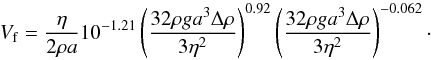 (A.5)
(A.5)
Appendix A.2: High Knudsen number
In the free-molecular regime, calculations have been made by Probstein (1968) leading to an expression for the drag coefficient: 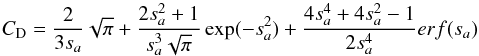 (A.6)
(A.6)
where sa is the ratio of the object velocity over the thermal speed of the gas (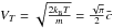 where
where  is the sound speed) and erf is the error function.
For velocities much smaller than the sound speed, sa → 0 and we can use an equivalent of the error function in 0: 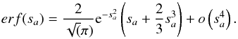 (A.7)Using this equation inside Eq. (A.6)and taking the limit sa → 0, the term e−sa2 goes to 1 and the terms proportional to
  cancels out leading to:
 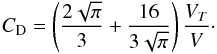 (A.8)For velocities much greater than the sound speed, the limit of Eq. (A.6)when sa → ∞ is:
  (A.9)In order to simplify Eq. (A.6)we use the following expression for the drag coefficient at high Knudsen number:
 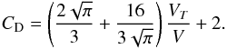 (A.10)Our approximation fits correctly the exact expression in the limit of low and high velocities. In between the difference to the exact expression is at most 30%. Replacing CD by its value in Eq. (A.2)we obtain a second order equation for the velocity:
 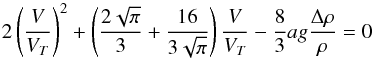 (A.11)which leads to:
 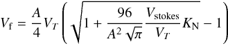 (A.12)with
  . When the speed becomes small compared to the sound speed (Vstokes ≪ VT) we obtain:
  (A.13)which is in good agreement with Eq. (3), derived for high Knudsen number and small Reynolds numbers.
Appendix A.3: Comparison with the Cunningham velocity
Figure A.1 shows the ratio of the Cunningham velocity (see Eq. (3)) to the ones we just derived. The difference is noticeable only for particles of the order of 100 μm at pressures less than the 10-4 bar level and exceeding the 10 bar level. This difference is always less than one order of magnitude and concern only a tiny portion of the parameter space which has little relevance to our study (the largest particle sizes considered in our 3D models is 10 μm). Thus we decided to neglect this discrepancy in the main study.
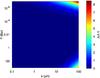 |
Fig. A.1
Ratio of the Cunningham velocity to the more sophisticated model of the particle settling velocity considered in the Appendix. |
| Open with DEXTER | |
© ESO, 2013
Current usage metrics show cumulative count of Article Views (full-text article views including HTML views, PDF and ePub downloads, according to the available data) and Abstracts Views on Vision4Press platform.
Data correspond to usage on the plateform after 2015. The current usage metrics is available 48-96 hours after online publication and is updated daily on week days.
Initial download of the metrics may take a while.