| Issue |
A&A
Volume 554, June 2013
|
|
|---|---|---|
| Article Number | A33 | |
| Number of page(s) | 26 | |
| Section | Extragalactic astronomy | |
| DOI | https://doi.org/10.1051/0004-6361/201321209 | |
| Published online | 31 May 2013 | |
Online material
Appendix A: Red clump peak variances
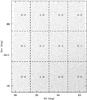 |
Fig. A.1
Field 6_6 split into a 4 × 3 array for analysis of RC variance (shown in Fig. A.2). Region names labelled. |
| Open with DEXTER | |
We analyse how the RC varies across the tile by splitting the tile into a 4 × 3 array (12 regions; shown in Fig. A.1). We locate the CMD area of highest density, corresponding to the most populated bin (using the same bin sizes as before: 0.01 mag in J − Ks and 0.05 mag in Ks; this limits their accuracy) and compare this with the median for colour and magnitude for each region; the values are in Table A.1. Figure A.2 shows the histogram distribution of the RC stars
in colour (top) and magnitude (bottom). For each region the normalised (with respect to the peak) average of regions 0 − 0 and 3 − 2 are overplotted in dashed red as a low extinction comparison. From this, it is seen that the regions with higher median colours have their source distribution extended in the redder component rather in addition to a complete offset (i.e. they are positively skewed). This suggests for a given region not all of the stars are affected by reddening but there is a multi-layer structure with some stars lying in front of the cause of the extinction. When comparing the contour peaks, which mirror the histogram peaks, to the median values, the difference is generally larger when the extinction is higher. The clearest example of this effect is in region 1 − 1 where 30 Doradus lies with a difference of 0.067 mag. Regions found to the north-west and south (1 − 0, 0 − 1, 0 − 2, 1 − 2) have similar difference. All these regions have strong H i and Hα emissions which may be related to the cause of this effect.
Red clump peak position across field 6_6 from median in CMD region and contour map peak position.
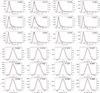 |
Fig. A.2
Histograms of the (J − Ks) colour (top 3 rows, bin size of 0.01 mag) and Ks magnitude (bottom 3 rows, bin size 0.05 mag) across the field (regions in parentheses defined in Table A.1). Value in top-right is the median. Overplotted in red is the normalised mean of regions 0 − 0 and 3 − 2. |
| Open with DEXTER | |
Appendix B: Extinction laws
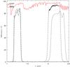 |
Fig. B.1
Comparison of wavelength vs. efficiency for the transmission of UKIRT (IRCAM3) J and K filters (in grey) and VISTA J and Ks filters (in dashed black). Curves from JAC and ESO, respectively. Synthetic spectra of a typical RC star in red. |
| Open with DEXTER | |
In Sect. 3.6 we mentioned that there are alternative extinction laws that could have been used instead (or rather, would have to have been used had the E(J − Ks) coefficients not already been calculated for our data in a model independent way). Here, we discuss these in more detail.
Table 6 of Schlegel et al. (1998) gives AJ/AV = 0.276 and AK/AV = 0.112. Therefore, E(J − K) = 0.164 × AV. These Schlegel et al. values are for JHK for UKIRT’s IRCAM3, while our observations are in VISTA YJKs. Both the UKIRT and VISTA photometry are in a Vega magnitude system.
However, UKIRT’s IRCAM3 and VISTA have different filter curves and system transmissions in detail, particularly in K/Ks. This causes the post-calibration magnitudes to vary slightly. In Fig. B.1, the filter curves and synthetic spectra of a RC star are shown (produced using model atmospheres from Castelli & Kurucz 2004). The J band widths are very similar, the main difference being at about 1.27 μm where the VISTA transmission
dips while the UKIRT one rises. The Ks passband curve begins before the K passband, finishes before it and the overall width is nearly identical. The extinction coefficients do vary slightly with spectral type (van Loon et al. 2003). This variance is small in the NIR (0.004 mag from A0 to M10 star in the J band).
The λeff and central wavelength values are given in Table B.1. The ratios to AV are derived from the RV = 3.1 curve meaning the AKs/AV value is derived using Eqs. (1), (2a) and (2b) in Cardelli et al. (1989); the results are shown in the rightmost column of Table B.1.
Using the VISTA values the conversion becomes E(J − Ks) = 0.1627 × AV, a difference of ~0.01 mag with band-by-band differences of ~ 0.05 mag when comparing the two systems. A drawback of this method is that it assumes the filter is well represented by the λeff point, rather than taking the full filter transmission curve into account. When comparing with the result from Sect. 3.6; E(J − Ks) = 0.16237 × AV, we see this simplification has had a rather small effect on the conversion, finding 102% of the used value and a maximum AV difference of ~−0.013 mag.
Some of the difference between UKIRT and VISTA values might be accounted for by how the λeff is calculated because the VISTA λeff values were calculated using Eq. (3) of Fukugita et al. (1996) (which was defined in Schneider et al. 1983) and accounting for the Quantum Efficiency curve while Schlegel et al. (1998) did not state how the UKIRT λeff was calculated (only that it represents the point on the extinction curve with the same extinction as the full passband).
Extinction ratio Aλ/AV for VISTA passbands.
Appendix C: Using the Y band
Figure C.1 shows a CMD of Ks mag vs. (Y − Ks). It is very similar to the Ks vs. (J − Ks) CMD seen in Fig. 3 with the difference of an extended colour axis due to a larger wavelength difference between the two bands. Focusing on the region of the RC we overplot the isochrones used in Sect. 3.5. This is shown in Fig. C.2. We see that the older isochrones lie bluer than the RC. This confirms, as expected, that the Y band is more affected by extinction towards the MCs than J or Ks are. When applying AV = 0.249 mag (Schlegel et al. 1998) as foreground Galactic extinction the (Y − Ks) and (J − Ks) are in a consistent position in the context of the contour levels (around the 35% level). This shows that the Y band, being closer to optical is more affected by extinction which would be a boon for low extinction regions because the contrast between extinctions would be greater. However, for a high extinction region it offers no advantage and has the disadvantage of stars being fainter in Y than in Ks. Colour–colour diagrams do not aid in selection of RC stars.
The RC selection box is defined like it is in Sect. 3.3. For (Y − Ks) the reddening vector is shallower (with a gradient of 0.5) and the colour limits are 0.75 < (Y − Ks) < 2 mag. Combined with an intrinsic colour of E(Y − Ks)0 = 0.84 mag and E(Y − Ks) = 0.2711 × AV the furthest we can probe is AV = 4.28 mag. The histogram for the RC selection is shown in Fig. C.3. Comparing with Fig. 9 we see the peak is at a slightly higher AV in the selection (due to greater foreground Galactic extinction probed). The percentage of stars relative to the peak at AV = 1 mag and AV = 2 mag is very similar in both histograms.
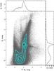 |
Fig. C.1
Ks vs. (Y − Ks) CMD of LMC field 6_6 accompanied by cyan contours representing density and histograms of (Y − Ks) (bin size 0.01 mag) and Ks (bin size 0.05 mag). It can be seen that this field is largely made up of main sequence and RC stars. |
| Open with DEXTER | |
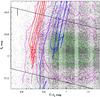 |
Fig. C.2
(Y − Ks) vs. Ks CMD with isochrone lines for the helium burning sequence for the same two metallicities and age ranges as Sect. 3.5. Younger, more metal rich (log (t/yr) = 9.0−9.4, Z = 0.0125) are in blue and the older, more metal poor (log (t/yr) = 9.4−9.7, Z = 0.0033) are in red. Error bars represent error in LMC distance. Contours are plotted in magenta and green and have the same levels as in Fig. 4. The older population can be seen to be at the 5% contour level. |
| Open with DEXTER | |
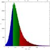 |
Fig. C.3
Histogram of E(Y − Ks) (bottom) and AV (top) distribution with bin size of 0.005 mag. Green is the region covering 50% of the sources centred on the median where darker blue is lower than this and brighter red higher and purple extremely high. |
| Open with DEXTER | |
© ESO, 2013
Current usage metrics show cumulative count of Article Views (full-text article views including HTML views, PDF and ePub downloads, according to the available data) and Abstracts Views on Vision4Press platform.
Data correspond to usage on the plateform after 2015. The current usage metrics is available 48-96 hours after online publication and is updated daily on week days.
Initial download of the metrics may take a while.