| Issue |
A&A
Volume 554, June 2013
|
|
|---|---|---|
| Article Number | A71 | |
| Number of page(s) | 16 | |
| Section | Planets and planetary systems | |
| DOI | https://doi.org/10.1051/0004-6361/201220680 | |
| Published online | 05 June 2013 | |
Online material
Best-fitting values of physical parameters determined for the B-types with WISE observations.
Best-fitting values of physical parameters determined for the Pallas collisional family asteroids excluding (2) Pallas with WISE observations.
Appendix A: Thermal modelling of WISE asteroid data
Our aim is to model the observed asteroid flux as a function of several physical parameters and derive the set of parameter values that most closely reproduce the actually measured fluxes. In this work we follow the method described by Mainzer et al. (2011b). The set of wavelengths covered by WISE (specified in Sect. 2) allow us to derive up to three parameters by fitting a thermal model to asteroid WISE data: asteroid effective diameter, beaming parameter, and reflectance at 3.4 μm (defined below). Within the wavelength range covered, the observed asteroid flux consists of two components:  (A.1)The thermal flux component (fth,λ) is the main contribution to W3 and W4, whereas the reflected sunlight component (rs,λ) dominates in band W1. In general, W2 will have non-negligible contributions from both components (Mainzer et al. 2011b).
The computation of fth,λ is based on the Near Earth Asteroid Thermal Model (NEATM; see Harris 1998; Delbó & Harris 2002). The asteroid is assumed to be spherical, and its surface is divided into triangular facets that contribute to the total thermal flux observed by WISE in accordance with the facet temperature (Ti), the geocentric distance (Δ), and the phase angle (α⊙). In turn, the temperature of each facet depends on the asteroid heliocentric distance (r⊙) and its orientation with respect to the direction towards the sun. It is given by  (A.2)which results from assuming that each surface element δai is in instantaneous equilibrium with solar radiation. S⊙ is the solar power at a distance of 1 AU, A the bolometric Bond albedo, ϵ the emissivity (usually taken to be 0.9; see Delbó et al. 2007, and references therein), σ the Stefan-Boltzmann constant, and μi = cosθi, where θi is the angle between the normal to the surface element i and the direction towards the Sun. Non-illuminated facets will be instantaneously in equilibrium with the very low temperatures of the surroundings (~0 K), and thus their contribution to fth,λ is neglected in the NEATM. Finally, the beaming parameter (η) can be thought of as a normalisation or calibration factor that accounts for the different effects that would change the apparent day-side temperature distribution of the asteroid compared to that of a perfectly smooth, non-rotating sphere (Harris 1998). These include, for example, the enhanced sunward thermal emission due to surface roughness (η < 1), or the non-negligible night-side emission of surfaces with high thermal inertia that, in order to conserve energy, causes the day-side temperature to be lower than that compared to the ideal case with zero thermal inertia (η > 1).
The asteroid thermal flux component is then given by  (A.3)where fi,λ is the contribution from each illuminated facet of a 1-km sphere; Ω ≡ (D/1 km)2 scales the cross-section of the latter to the corresponding value of an asteroid of diameter D. The colour correction associated with each value of Ti and each WISE band is applied to the facet flux. By definition, it is the quotient of the in-band flux of the black body at the given temperature to that of Vega (Wright et al. 2010). A colour correction table was generated for all integer temperatures from 70 K up to 1000 K using the filter profiles available from Cutri et al. (2012).
The reflected light component, the second term on the right-hand side of Eq. (A.1), is calculated as follows. First, the asteroid visible magnitude (V) that would be observed at a given geometry (r⊙, Δ and α⊙) can be estimated using the IAU phase curve correction (Bowell et al. 1989), along with the tabulated values of asteroid absolute magnitude (H) and slope parameter (G) from the Minor Planet Center. Secondly, knowledge of the solar visible magnitude and flux at 0.55 μm (V⊙ and fV⊙, respectively) allows us to calculate the sunlight reflected from the asteroid at that particular wavelength:  (A.4)If we assume that the Sun is approximated well by a black-body emitter at the solar effective temperature (T⊙ = 5778 K), the estimated reflected flux at any other desired wavelength (rλ) can be computed by normalising the black body emission Bλ(T⊙) to verify rV, i.e.
 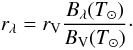 (A.5)In this approximation, we can also consider
 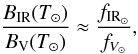 (A.6)from which we arrive at the following expression:
 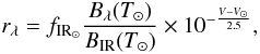 (A.7)where the subscript IR denotes 3.4 μm. We do not colour-correct this component given the small correction to the flux of a G2V star (see Table 1 of Wright et al. 2010). Finally, to account for possible differences in the reflectivity at wavelengths longward of 0.55 μm, a prefactor to rλ is included in the model, such that
  (A.8)This prefactor, Rp, is by definition equivalent to the ratio of pIR and the the visible geometric albedo, so we will refer to it as the “albedo ratio”. The paremeter pIR is the reflectivity at 3.4 and 4.6 μm defined by Mainzer et al. (2011b).
To sum up, the observed model flux can then be written as 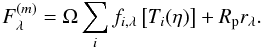 (A.9)We use the Levenberg-Marquardt algorithm (Press et al. 1986) in order to find the values of asteroid size (
 , in km), beaming parameter (η) and albedo ratio (Rp) that minimise the χ2 of the asteroid’s WISE data set, namely
  (A.10)where Fj,λ and σj,λ are the measured fluxes and corresponding uncertainties, j runs over the observation epochs, and λ labels the WISE bands. The implementation of this technique involves calculating the partial derivatives of
  with respect to the fitting parameters, which is straightforward in the case of Ω and Rp. The partial derivative with respect to η can be derived from
  (A.11)
Appendix B: Comparison with Masiero et al. (2011)
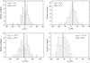 |
Fig. B.1
Fractional difference histograms of D, η, pV, and Rp. We define ε = 100(x − xM)/x, where x is the parameter value in this work and xM the correspoding value taken from Table 1 by Masiero et al. (2011). The vertical lines mark the corresponding average values. Only parameters resulting from the same input values of H contribute to these histograms. |
| Open with DEXTER | |
Figure 2 shows that our parameter determinations and those of Masiero et al. (2011) are compatible in spite of the slight differences in the data set and the thermal modelling used in this work (refer to Sect. 2 and Appendix A), from which we do not expect to obtain exactly the same best-fit parameters for each object. In order to carry out a detailed comparison between our results and those of Masiero et al. (2011), we computed the mean fractional difference (ε) and corresponding standard deviations of D, η, pV, and Rp. Let ε = 100(x − xM)/x, where x is the parameter value for a given object in this work, and xM the correspoding value taken from Table 1 by Masiero et al. (2011). The distributions of ε values are plotted in Fig. B.1. These histograms only include parameter determinations that have the same H as input in order to identify possible discrepancies in results not caused by different values of H. We find that our values of D and η tend to be slightly higher by 1% and 3%, respectively, whereas our pV values are lower by 2%, though these deviations are small compared to the error bars. On the other hand, there is a large bias towards lower values of Rp that, while still being within the error bar, must be addressed.
Most probably, the Rp discrepancy is associated with how the reflected flux rλ is calculated. In particular, we take the solar flux at 3.4 μm (fIR⊙ in Eq. (A.7)) from the solar power spectrum at zero air mass of Wehrli4, based on the one by Neckel & Labs (1984). Any differences in input, including solar visible magnitude, taken from tabulated data sources that may cause our rλ to be systematically 10% greater than that of Masiero et al. (2011) would explain our higher values of Rp. For instance, considering that there is only one optimum value of rs,λ to fit a given W1 data set, from Eq. (A.8) it is clear that larger rλ will have associated a lower best-fit value of Rp.
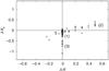 |
Fig. B.2
Differences in albedo ratio determinations versus difference in absolute magnitude corresponding to the B-types in this paper and those by Masiero et al. (2011). |
| Open with DEXTER | |
The Monte Carlo estimations by the NEOWISE team show that the error bars associated to the fitting of the data are always small compared to the errors inherent to the thermal model itself. The relative errors in diameters derived from the NEATM have been characterised as ~10%–15% (Harris 2006). From these facts and the widths of the ε-value distributions of Fig. B.1, we consider it safe to assume a minimum relative error of 10% in diameter and 20% in beaming parameter, pV and Rp. On the other hand, large uncertainties in the absolute magnitude (sometimes as large as ~0.3 mag) will also affect the values of pV, so 20% is probably an optimistic assumption in some cases.
Finally, we also evaluate how differences in the values of H result in different values of pV and Rp. We downloaded the MPC orbital element file as of May 2012 and compared the values of absolute magnitude (HU) to those used by Masiero et al. (2011), HM. About 50000 H-values have been updated between these two works, and ~38 000 have been enlarged. Figure 1 shows a histogram of ΔH ≡ HU − HM for the B-types in this work. Out of the 52 objects with ΔH ≠ 0, as many as 43 of them have ΔH > 0. Our size determinations agree to within 10%, therefore higher updated values of H will result in lower values of geometric albedos.
In Fig. B.2 we show a plot of ΔRp ≡ Rp − (Rp)M versus ΔH for all the B-types with determined values of Rp. The notation (Rp)M refers to the corresponding albedo ratios by Masiero et al. (2011). There are three features to note in this plot: (1) our values of Rp tend to be ~10% systematically lower, as we already noted (see Fig. B.1); (2) most points off the ΔH = 0
axis show a direct correlation between ΔRp and ΔH, as expected from the discussion above; (3) some points show ΔRp < −0.5, even though ΔH = 0. The points of feature (3) are explained by an inconsistency in the pV values of Masiero et al. (2011) with their corresponding values of D and H: they do not verify Eq. (1) and are always lower than the predicted pV.
To sum up, we have shown that if the input values of H are equal, our model fits are consistent within the model error bars with those presented in Table 1 of Masiero et al. (2011). The tendency to 10% lower values of Rp is likely caused by differences in solar power spectra data taken to estimate the reflected light component at NIR wavelengths (see Eq. (A.7)). We have also examined how updated input values of H affect the best-fit parameter values and showed how increasing the value of H results in greater values of Rp and vice versa.
© ESO, 2013
Current usage metrics show cumulative count of Article Views (full-text article views including HTML views, PDF and ePub downloads, according to the available data) and Abstracts Views on Vision4Press platform.
Data correspond to usage on the plateform after 2015. The current usage metrics is available 48-96 hours after online publication and is updated daily on week days.
Initial download of the metrics may take a while.