| Issue |
A&A
Volume 553, May 2013
|
|
|---|---|---|
| Article Number | A73 | |
| Number of page(s) | 17 | |
| Section | The Sun | |
| DOI | https://doi.org/10.1051/0004-6361/201220463 | |
| Published online | 07 May 2013 | |
Online material
Appendix A: Effects of spectral broadening
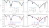 |
Fig. A.1
Convolution of the FAL NLTE profiles with different spectral PSFs. Bottom: convolution of FAL-C with Gaussians of σ = 3.4 pm (blue line) and 9.4 pm (purple line). The black line shows the observed average QS profile. Left column: line wing. Right column: line core. Top: convolution of FAL-A with a wavelength-dependent Gaussian with σ between 3.4 and 9.4 pm. |
| Open with DEXTER | |
The effective spectral resolution of the POLIS spectrograph can lead to a loss in amplitude of the emission peaks by spectral smearing because of their small spectral extent. The default spectral resolution of POLIS is 220.000@400 nm (≡1.8 pm), but because of the on-chip binning by a factor of two, the resolution is sampling-limited to about 3.8 pm. Convolving an FTS (Kurucz et al. 1984) reference spectrum with the method of Allende Prieto et al. (2004) and Cabrera Solana et al. (2007) to match the observed average Ca profile yielded the need for a Gaussian with σ ~ 1.7 pm. We note that the FTS spectrum contains line broadening by macroturbulent velocities because of being a spatially averaged QS spectrum.
For an estimate of the maximal spectral smearing between the observed average QS profile and the FAL-C NLTE profile − synthesized without a macroturbulent velocity – by instrumental effects, we first convolved the FAL-C NLTE profile as reference by a Gaussian to match the shape and width of the line blends in the Ca line wing in the average observed spectrum. The lower-left panel of Fig. A.1 shows that this requires a value of σ of about 3.4 pm, which is in rough agreement with the prediction from the sampling limit. A convolution of the full spectrum with this value as an estimate of the instrumental and velocity broadening in the atmosphere reduces, however, the amplitude of the emission peaks of the FAL-C NLTE profile only slightly (lower-right panel of Fig. A.1). To force the emission peaks in the synthetic profile to a shape roughly resembling the observed profile requires a convolution of FAL-C with a Gaussian with σ = 9.4 pm. The line blends in the wing, however, clearly exclude such a large instrumental broadening because in the FAL-C NLTE profile convolved with σ = 9.4 pm (purple line) the blends are twice as broad and half as deep as in the observed spectrum (lower-left panel of Fig. A.1).
We then decided to try a wavelength-dependent width of the Gaussian used as spectral point spread function (PSF). The width
was set to 3.4 pm in the line wing up to λ = 396.75 nm, gradually increasing to 9.4 pm at λ = 396.85 nm, and reducing down to 3.4 pm again at λ = 396.94 nm. As it seemed impossible to match the FAL-C NLTE and the observed profile even with a large broadening in the very core, we applied this variable convolution to the FAL-A NLTE profile instead. The temperature stratification of FAL-A has a weaker chromospheric temperature rise than FAL-C (Fig. 15) and the corresponding NLTE profile differs significantly from FAL-C, especially in the residual line-core intensity (Fig. 14). The approach with the variable spectral PSF maintains the match in the line wing (upper-left panel of Fig. A.1) and leads to an acceptable agreement between the emission peaks of the convolved FAL-A NLTE profile and the observed spectrum (upper-right panel).
The wavelength-dependent Gaussian spectral PSF would correspond to a microturbulent velocity vmic that changes from 2.6 km s-1 in the photosphere to 7.1 km s-1 in the chromosphere. The NLTE synthesis already included a height-dependent microturbulent velocity of more than 5 km s-1 for log τ < −5.5. Thus, the effective microturbulent velocity necessary to match the averaged observed and the FAL-A NLTE profile should be nearly twice as large as the initial value of vmic, and has to be present already at lower layers of log τ ~ −3 to yield the correct shape of the H1V and H1R minima next to the emission peaks. We note that similar values of vmic would be also required to match the FTS atlas and the FAL-A NLTE profile, because the line shape in the FTS is similar to the average QS spectra shown here. Whether such a high value of vmic is reasonable for spectra at about 1′′ spatial resolution needs further investigation. Additionally, the increase in vmic at comparably low layers of log τ also already affects the Fe i line blend at 396.93 nm strongly, broadening it significantly beyond its width in observed spectra. Doubling vmic therefore seems not to be a valid option to match observed and theoretical NLTE profiles, leaving a reduction of temperature as the only option (cf. Rezaei et al. 2008).
© ESO, 2013
Current usage metrics show cumulative count of Article Views (full-text article views including HTML views, PDF and ePub downloads, according to the available data) and Abstracts Views on Vision4Press platform.
Data correspond to usage on the plateform after 2015. The current usage metrics is available 48-96 hours after online publication and is updated daily on week days.
Initial download of the metrics may take a while.