| Issue |
A&A
Volume 552, April 2013
|
|
|---|---|---|
| Article Number | A114 | |
| Number of page(s) | 8 | |
| Section | The Sun | |
| DOI | https://doi.org/10.1051/0004-6361/201220512 | |
| Published online | 11 April 2013 | |
Online material
Appendix A: Model description
The annual solar Strömgren (b + y)/2 flux values F(t) can be decomposed into the long-term FLT(t) and cyclic F11(t) components (see, e.g. Tapping et al. 2007) 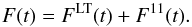 (A.1)While cyclic component F11(t) varies on the 11-year time scale and controls the activity cycle, the long-term component FLT(t) varies on secular time scales and leads to a changeable level of the flux during the solar activity minima.
Most of the stars in the Lockwood et al. (2007) dataset are observed over an approximately 20-year period. Therefore, to compare stellar and solar variabilities we will introduce the rms20 value. For any given year t, it is the rms variability of the dataset which consists of twenty annual flux values (from year t−9, till year t + 10).
The total variability of the solar flux can be calculated as the geometrical sum of the long-term and cyclic variabilities  (A.2)We introduce parameter V11 as rms variability of the annual (b + y)/2 flux values for the 1976–1996 period (solar cycles 21 and 22). The Krivova et al. (2010), Shapiro et al. (2011), and Lean et al. (2005) reconstructions show the value of V11 parameter equals 0.00019 mag, 0.00018 mag, and 0.000032 mag, respectively.
To calculate the cyclic component backwards in time, we assume that its amplitude is proportional to the long-term solar activity φ(t). The latter can be reconstructed over the millennia from the cosmogenic isotope data, which gives a 22-year running mean of the modulation potential (Steinhilber et al. 2008; Herbst et al. 2010). Thus, the cyclic rms variability for any given year t can be calculated as 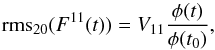 (A.3)where φ(t) is the modulation potential and φ(t0) is the mean value of the modulation potential for the 1976–1996 period. The modulation potential is deduced from the composite of the neutron monitor data (Usoskin et al. 2005) and 10Be data (McCracken et al. 2004; Vonmoos et al. 2006). It is normalised to the Castagnoli & Lal (1980) local interstellar spectra. The homogenisation procedure is discussed in Shapiro et al. (2011) and Thuillier et al. (2012). The average uncertainty of the modulation potential changes is ~80 MeV (Vonmoos et al. 2006) and does not have a significant contribution to the temporary mean of the solar variability.
To calculate the rms20(FLT(t)) contribution we introduce parameter VLT as a relative change of FLT between the present and the Maunder minimum. The changes of the solar flux between three recent solar minima are within the uncertainties of the reconstructions and measurements of the solar irradiance (see review by Ermolli et al. 2012), so the FLT component can be approximated by a constant for the last solar cycles. Therefore, for simplicity we define VLT as the relative change of the (b + y)/2 flux between the 1996 and the Maunder minima.
We assume that the long-term changes of the solar irradiance are proportional to the changes of the solar activity φ(t)  (A.4)where t0 refers to our reference period (1976–1996 average) and tM refers to the Maunder minimum.
Substituting FLT(tM) − FLT(t0) = VLT FLT(t0), one can connect the relative changes of the solar flux and activity  (A.5)Equation (A.5) links rms20(FLT(t)) and rms20(φ(t)) via the parameter VLT. In combination with Eqs. (A.2) and (A.3) it allows one to reconstruct the solar variability backwards in time as a function of V11 and VLT parameters.
The approach, presented above is based on three assumptions:
-
1.
The amplitude of the activity cycle is proportional to thelong-term (i.e. cycle-averaged) solar activity.
-
2.
The long-term changes of the solar irradiance are proportional to the long-term changes of the solar activity.
-
3.
The long-term solar activity can be reconstructed from the cosmogenic isotope data.
Let us note that these assumption are either employed or fulfilled because of the physical reasons in most of the available reconstructions, independently from the proposed mechanism for the secular changes.
To estimate the accuracy of our approach we consider three different reconstructions of the solar irradiance to the past: Krivova et al. (2010) (VLT = 0.044%, V11 = 0.000019 mag), Shapiro et al. (2011) with removed long-term trend (VLT = 0%, V11 = 0.000018 mag), and the original Shapiro et al. (2011) reconstruction (VLT = 0.38%, V11 = 0.000018 mag). They yield 0.0001 mag, 0.00009 mag, and 0.00036 mag for the mean solar rms20 variability over the 1620–1995 period. The same values calculated with the set of Eqs. (A.2)–(A.5) are 0.00013 mag, 0.00012 mag, and 0.00035 mag. One can see that our approach slightly overestimates the first two numbers. The reason for this is that to allow a homogeneous reconstruction over the millennia we use the solar modulation potential to scale the cyclic variability (see Eq. (A.3)) instead of the sunspot number. The annual sunspot number is very close to zero during the Maunder minimum period, so the reconstructions predict the cessation of the cyclic variations (see Fig. 2). At the same time the modulation potential and consequently the cyclic variability in our approach did not go to zero during the Maunder minimum (McCracken et al. 2004). Such deviations are comparable to the uncertainties of the reconstructions and are not essential for our conclusions.
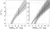 |
Fig. B.1
Left panel: the dependency of the VLT parameter on the solar variability, retrieved from the stellar data. The shaded area indicates the uncertainty (2σ) due to the limited number of stars. The V11 parameter is set to 0.00044 mag. The dashed line corresponds to the expected mean solar variability rms20 = 0.00082. The projection onto VLT-axis yields the 95% interval for expected long-term variability of the Sun: 0.43% < VLT < 0.76%. Right panel: the same as the left panel, but the contour calculated with V11 = 0.0002 mag is added. The four dashed lines correspond to four values of expected mean solar variability rms20: 0.00097 mag (no chromospheric secular changes, regression with solid line from Fig. 1), 0.00082 mag (strong chromospheric secular changes, regression with solid line), 0.00065 mag (no chromospheric secular changes, regression with dashed line), 0.00053 mag (strong chromospheric secular changes, regression with dashed line). The projection onto the VLT-axis yields the interval 0.17% < VLT < 1.2%. |
| Open with DEXTER | |
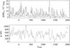 |
Fig. B.2
Upper panel: rms20 back to 400 BC, adopting VLT = 0.001 (lower curve) and VLT = 0.005 (upper curve). V11 is set to 0.0002 mag. Lower panel: modulation potential back to 400 BC. The interval in the upper-right corner denotes the satellite era of continuous solar irradiance measurements. |
| Open with DEXTER | |
The calculation of the Ca II H and K lines, which are used to determine the solar chromospheric activity, made even more complicated by the effect of the non-local thermodynamical equilibrium (Ermolli et al. 2010). So the mean solar chromospheric activity cannot be directly deduced from the available reconstructions of the solar irradiance over the millennia. Instead we will linearly scale it with the long-term solar activity  (A.6)where
  is the present value of the mean solar chromospheric activity (
 , see Lockwood et al. 2007) and
  is the value of the mean chromospheric activity corresponding to φ = 0.
In Fig. 3 we consider two extreme scenarios (see Sect. 3), one without the secular component in the solar chromospheric activity, and another with a strong secular component. Without the secular component the changes of the mean solar chromospheric activity are only caused by the variable amplitude of the solar activity cycle and the  value corresponds to the present value of the solar activity at minimum conditions (
 ; see Judge & Saar 2007). To describe the case of a strong secular component in the chromospheric activity we put the value equals to the boundary value from Saar (2006) (
 ).
).
Appendix B: Possible constraints on the historical solar variability
The amplitude of the secular solar photometric variability can be constrained by demanding the temporal mean solar variability be in agreement with the variability, indicated by the stellar data. The latter depends on the version of the variability versus activity regression and the scenario of the chromospheric activity behaviour. To investigatedifferent cases in Fig. B.1 we plot the long-term solar variability VLT as a function of the mean solar variability (rms20) given by the stellar data, for two values of the 11-year variability V11. The inclination effect was calculated according to Knaack et al. (2001).
Let us note, however, that the positions of the Sun-like stars in Fig. 3 are also not necessarily fixed in time. This can affect the coefficients of the regression line and accordingly the estimated variability of the Sun. For example it is possible that, by coincidence, most of the stars among the twenty-one used for our analysis represent the periods of the relatively low (or high) variability. This will lead to the shifted position of the regression line and consequently to the deviations in the Vlt parameter determined using this limited selection of stars.
If the behaviour of the stellar variabilities after the regression to the solar level of the chromospheric activity is identical to the solar variability, i.e. the solar and regressed stellar variabilities can be parameterised employing the approach described in Sect. 3 and Appendix A, then the resulting uncertainty can be found by performing the Monte Carlo simulation. To do this we considered a large number of sets consisting of 21 stars. Every star in these sets represents the Sun at some random twenty-year interval period (chosen from the full 9000-year dataset) and with a random angle between the stellar rotation axes and the direction to the observer. The rms20 variability of these stars is calculated, employing the approach described in Sect. 3 and Appendix A and the Knaack et al. (2001) dependency of the 11-year variability on the angle between the solar rotation axes and the direction to the observer. For every set we calculated the mean rms20 variability of the stars in the set, so for every pair of VLT and V11 parameters we have a distribution of mean rms20 variabilities. This allows us to calculate the range of VLT and V11 parameters which can lead to the present value of the linear coefficients of the activity versus variability regression line. In Fig. B.1 we mark the resulting 2σ uncertainty in VLT parameter with a shaded area.
The mean solar  index in the case of the strong secular component in chromospheric activity is − 4.96 (see Fig. 3). Using the solid blue line in Fig. 1 one can find that this index corresponds to the 8.2 × 10⁻⁴ rms variability. This value is inserted in the left panel of Fig. B.1 and one can see that it yields VLT = (0.43%−0.76%).
In the right panel of Fig. B.1 we also plotted the contour with V11 = 0.0002 mag and indicated four different values of the expected solar variability, corresponding to different treatments of the chromospheric secular changes and two regressions from Fig. 1. One can see that the minimum value of VLT equals 0.17%.
The parameter VLT characterises the long-term variability as it is observed in the Strömgren b and y filters. Its connection with the variability at another spectral domain (or TSI) depends on the mechanism of the secular changes. For example a VLT equal to 0.17% leads to a 2.7 W/m2 TSI change between the Maunder and the last solar minima, adopting the model of Shapiro et al. (2011), and to 1.9 W/m2, assuming that it is caused by the variations of the solar effective temperature.
© ESO, 2013
Current usage metrics show cumulative count of Article Views (full-text article views including HTML views, PDF and ePub downloads, according to the available data) and Abstracts Views on Vision4Press platform.
Data correspond to usage on the plateform after 2015. The current usage metrics is available 48-96 hours after online publication and is updated daily on week days.
Initial download of the metrics may take a while.