| Issue |
A&A
Volume 549, January 2013
|
|
|---|---|---|
| Article Number | L6 | |
| Number of page(s) | 7 | |
| Section | Letters | |
| DOI | https://doi.org/10.1051/0004-6361/201220668 | |
| Published online | 21 December 2012 | |
Online material
Appendix A: Data reduction details
For extended emission – as seen in CO J = 6−5 towards IRAS 16293 – the uv sampling density towards short baselines is crucial for a successful recovery of large spatial scales. In the image reconstruction process, each baseline contributes a corrugation pattern along a position angle in the image plane that corresponds to the position angle of the antenna pair in the uv plane. Amplitude and position of this wave-like pattern are determined by its complex visibility. A single baseline, therefore, does not provide enough information to constrain the spatial origin of the emission. The combined information of many antenna pairs with various baseline lengths and position angles is required to get an image with genuine structures.
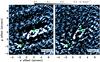 |
Fig. A.1
Channel maps at −3 km s-1 before and after additional flagging (see
text). The offsets are as in Fig. 1. The
color scale ranges from 0 to 0.3 Jy beam-1
(0 to ~3σ) and has been chosen to highlight the striping
present in the left map (original data) but not the right (flagged data). The blue
contours are at 1σ in this 0.25 km s-1 channel. The
red dot at (0 |
| Open with DEXTER | |

This also means that if a certain region in the uv plane is under-sampled, this will lead to imaging artifacts. To a certain degree these can be removed during the image deconvolution process. However, if an under-sampled baseline exhibits strong correlated flux density, the corrugation pattern, which is caused by this antenna pair, will remain in the deconvolved image and might be misinterpreted as real structure. For this reason we flag the baseline DA47&DV14, which is the only one that samples spatial scales above 3′′. Since this baseline exhibits high correlated flux densities, the reconstructed image shows a clear corrugation pattern, which is indicative of extended structures that cannot be quantified correctly (Fig. A.1).
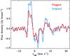 |
Fig. A.2
Spectrum towards a position located along the blue arch and marked in Fig. A.1. The flagged and original data are shown in red and blue, respectively. |
| Open with DEXTER | |
Additional analysis of the visibilities lead to the flagging of the antenna pair DA41&DV09. We made use of the fact that two execution blocks were observed almost exactly 24 h apart, leading to almost identical uv coverage. This made it possible to cross check the visibilities. In certain channels at blue-shifted velocities, DA41&DV09 exhibited strong correlated flux densities, but with significant differences between the two execution blocks.
The flagging of these two baselines significantly changed the spectra at certain positions in the sky (see Fig. A.2 for an example), particularly at positions associated with the blue arch. We suspect that large-scale structure (>3′′) is associated with the blue arch, but that full ALMA is required to recover it (with the Atacama Compact Array, ACA, and Total Power, TP, telescopes included). We note that the overall morphology of the system has not changed, and all key structures can be recovered although the blue arch appears to sit on a plateau of emission at velocities of ~3 km s-1 in the original data (Fig. A.1).
Appendix B: Comparison of outflow emission at sources A and B
We illustrate below that if the arch were caused by source B, instead of being a chance
alignment, a very different outflow collimating structure would be
required to that found in source A. We do so by assuming that the opacity towards the
continuum peaks of sources A and B are the same ( =
=
 = τ)
and that the line emission source functions are the same
(
= τ)
and that the line emission source functions are the same
( =
=
 = Sv)
towards both continuum peaks, but that only a fraction, f, of the
emission will be recovered by the interferometer. This fraction may be different towards
the two sources, and we denote the fraction recovered towards source A
with f and towards source B
with ηf. Only in the case where the outflow structure
at the base of the outflow (i.e., at the continuum peak) is similar towards the two
sources is η = 1.
= Sv)
towards both continuum peaks, but that only a fraction, f, of the
emission will be recovered by the interferometer. This fraction may be different towards
the two sources, and we denote the fraction recovered towards source A
with f and towards source B
with ηf. Only in the case where the outflow structure
at the base of the outflow (i.e., at the continuum peak) is similar towards the two
sources is η = 1.
The standard equation of radiative transfer reads:
 (B.1)where
Iv(0) is the continuum contribution.
Towards sources A and B, respectively, the radiative-transfer equations become:
(B.1)where
Iv(0) is the continuum contribution.
Towards sources A and B, respectively, the radiative-transfer equations become:
 (B.2)
(B.2) (B.3)When moving into the
blue-shifted line wing towards source A, the line emission decreases until almost
nothing is left but the continuum:
(B.3)When moving into the
blue-shifted line wing towards source A, the line emission decreases until almost
nothing is left but the continuum:  (B.4)In other words,
line emission and absorption are balanced and it follows from Eq. (B.4) that
(B.4)In other words,
line emission and absorption are balanced and it follows from Eq. (B.4) that
 (B.5)The ratio of observed
emission towards sources B and A is
(B.5)The ratio of observed
emission towards sources B and A is  where
R =
where
R =  is the ratio of the
continuum emission towards the two peaks. The value of R is
3.05 Jy beam-1/ 1.13 Jy beam-1 = 2.69. Solving
for τ gives
is the ratio of the
continuum emission towards the two peaks. The value of R is
3.05 Jy beam-1/ 1.13 Jy beam-1 = 2.69. Solving
for τ gives  (B.9)The value of
τ can be estimated towards source B based on the available data.
If the absorption is caused entirely by a foreground layer,
τ = ln(Iv(0)/Iv)
which is shown in Fig. B.1. However, the arch is
primarily observed in emission around source B which means that this value
of τ is a lower limit because both emission and absorption needs to
be accounted for. Towards the deepest absorption feature, τ is greater
than 1.0−1.5. The observed intensity ratio,
(B.9)The value of
τ can be estimated towards source B based on the available data.
If the absorption is caused entirely by a foreground layer,
τ = ln(Iv(0)/Iv)
which is shown in Fig. B.1. However, the arch is
primarily observed in emission around source B which means that this value
of τ is a lower limit because both emission and absorption needs to
be accounted for. Towards the deepest absorption feature, τ is greater
than 1.0−1.5. The observed intensity ratio,  is
displayed in Fig. B.2. At the bottom of the
absorption feature, the emission ratio is ~0.5. Figure B.3 shows η as a function of τ for various
values of the emission ratio . For an
observed emission ratio of 0.5, η is at most 0.5, irrespective
of τ, which implies that at most ~50% of the emission recovered
towards source A is recovered towards source B at this velocity. If more emission were
recovered, the absorption feature would be filled with the emission.
is
displayed in Fig. B.2. At the bottom of the
absorption feature, the emission ratio is ~0.5. Figure B.3 shows η as a function of τ for various
values of the emission ratio . For an
observed emission ratio of 0.5, η is at most 0.5, irrespective
of τ, which implies that at most ~50% of the emission recovered
towards source A is recovered towards source B at this velocity. If more emission were
recovered, the absorption feature would be filled with the emission.
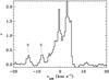 |
Fig. B.1
Line opacity, τ towards the continuum peak of source B. The unidentified line features are marked with U. The opacity is a lower limit as discussed in the text. |
| Open with DEXTER | |
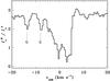 |
Fig. B.2
Line emission ratio from the peak of continuum emission towards source B and a line-free position near the peak of source A. The unidentified line features are marked with U. |
| Open with DEXTER | |
 |
Fig. B.3
η as a function of the line opacity for different emission ratios. The contours are at emission ratios of 0.2, 0.4, 0.6, ... to 2.0 with the four lowest ratios labeled. |
| Open with DEXTER | |
The above derivation is only valid if the bases of the outflows are similar. As Loinard et al. (2012) argue, source B may be a candidate first hydrostatic core in which case the outflow is expected to be less collimated and therefore may be subject to more filtering. However, for that to be the case, source B must be located at the apex of the arch. Figure B.4 shows a set of CO channel maps obtained at blue-shifted velocities. All four maps, and in particular those at −1.5 and −2.5 km s-1, show that source B is not at the apex of the arch. From these arguments we conclude that the blue arch is unrelated to source B and is a chance alignment in the plane of the sky.
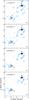 |
Fig. B.4
Channel maps of blue-shifted emission at the velocities indicated in the upper left corner of each panel. The channels have a width of 0.25 km s-1 and contours are at 4, 8, 12, ... σ. The background grayscale image is the continuum. The positions of sources A and B are marked. |
| Open with DEXTER | |
© ESO, 2013
Current usage metrics show cumulative count of Article Views (full-text article views including HTML views, PDF and ePub downloads, according to the available data) and Abstracts Views on Vision4Press platform.
Data correspond to usage on the plateform after 2015. The current usage metrics is available 48-96 hours after online publication and is updated daily on week days.
Initial download of the metrics may take a while.