| Issue |
A&A
Volume 545, September 2012
|
|
|---|---|---|
| Article Number | A120 | |
| Number of page(s) | 16 | |
| Section | Stellar atmospheres | |
| DOI | https://doi.org/10.1051/0004-6361/201219480 | |
| Published online | 18 September 2012 | |
Online material
Appendix A: Relativistic kinetic equation for Compton scattering and the RFs
For completeness let us rederive here the exact relativistic expressions for the Compton scattering RFs. For the detailed derivation, see Nagirner & Poutanen (1993) and Poutanen & Vurm (2010), where more general problems have been solved. In the first paper, the redistribution matrices describing Compton scattering of polarized radiation in terms of Stokes parameters were derived, while in the second the RFs for anisotropic electron distribution have been obtained. We start from the relativistic kinetic equation (RKE) for photons that describes Compton scattering.
A.1. Radiative transfer equation
A description of interactions between photons and electrons via Compton scattering
accounting for the induced scattering and electron degeneracy can be provided by the
explicitly covariant RKE for photons (Buchler &
Yueh 1976; de Groot et al. 1980; Nagirner & Poutanen 1993, 1994) 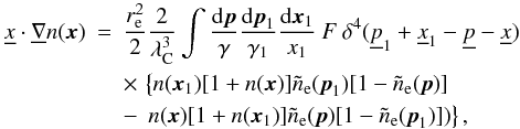 (A.1)where
 is the four-gradient,
re is the classical electron radius,
λC = h/mec is
the Compton wavelength, F is the Klein-Nishina reaction rate (Berestetskii et al. 1982)
is the four-gradient,
re is the classical electron radius,
λC = h/mec is
the Compton wavelength, F is the Klein-Nishina reaction rate (Berestetskii et al. 1982) 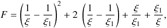 (A.2)and
  (A.3)are the
four-products of the corresponding momenta (second equalities in Eq. (A.3) arising from the four-momentum
conservation law represented by the delta-function in Eq. (A.1)). Here we define the dimensionless
photon four-momentum as
(A.3)are the
four-products of the corresponding momenta (second equalities in Eq. (A.3) arising from the four-momentum
conservation law represented by the delta-function in Eq. (A.1)). Here we define the dimensionless
photon four-momentum as 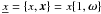 ,
where ω is the unit vector in the photon propagation
direction and
x ≡ hν/mec2.
The photon distribution is described by either the occupation
number n or the specific intensity (per dimensionless energy
interval)
I(x) = x3n(x)/C,
where the constant C is given by Eq. (13). The dimensionless electron four-momentum is
,
where ω is the unit vector in the photon propagation
direction and
x ≡ hν/mec2.
The photon distribution is described by either the occupation
number n or the specific intensity (per dimensionless energy
interval)
I(x) = x3n(x)/C,
where the constant C is given by Eq. (13). The dimensionless electron four-momentum is
 ,
where Ω is the unit vector along the electron
momentum, γ and
,
where Ω is the unit vector along the electron
momentum, γ and  are the electron Lorentz factor and its momentum in units
of mec, and β is the
velocity in units of c. The electron distribution is described by the
occupation number
are the electron Lorentz factor and its momentum in units
of mec, and β is the
velocity in units of c. The electron distribution is described by the
occupation number  .
For the isotropic electron distribution, we use the electron distribution function
.
For the isotropic electron distribution, we use the electron distribution function
 , normalized
to unity
, normalized
to unity  (A.4)In the following, we
consider a steady state and ignore electron degeneracy, because in the upper
atmosphere layers, where the radiation spectrum is formed, electrons are
non-degenerate. We define the RF as
(A.4)In the following, we
consider a steady state and ignore electron degeneracy, because in the upper
atmosphere layers, where the radiation spectrum is formed, electrons are
non-degenerate. We define the RF as  (A.5)For the relativistic
Maxwellian distribution of temperature
Θ = kTe/mec2
(Jüttner 1911; Synge 1957),
(A.5)For the relativistic
Maxwellian distribution of temperature
Θ = kTe/mec2
(Jüttner 1911; Synge 1957),  (A.6)(where
K2 is the modified Bessel function), the RF satisfies
the symmetry property
(A.6)(where
K2 is the modified Bessel function), the RF satisfies
the symmetry property  (A.7)which follows
from its definition in Eq. (A.5) and
the energy conservation
γ1 = γ + x − x1,
or from the detailed balance condition (see Eq. (8.2) in Pomraning 1973). Using this result it is easy to show that the
Bose-Einstein distribution
n(x) = 1/(exp { [x − μ] /Θ } − 1)
with any chemical potential is a solution of the RKE (A.1).
(A.7)which follows
from its definition in Eq. (A.5) and
the energy conservation
γ1 = γ + x − x1,
or from the detailed balance condition (see Eq. (8.2) in Pomraning 1973). Using this result it is easy to show that the
Bose-Einstein distribution
n(x) = 1/(exp { [x − μ] /Θ } − 1)
with any chemical potential is a solution of the RKE (A.1).
In the absence of strong magnetic field, the medium is isotropic, therefore the RF
depends only on the photon energies and the scattering angle (where η
is its cosine), i.e. we can write
R(x1 → x) = R(x,x1,η).
The kinetic Eq. (A.1) can then be
recast in a standard form of the radiative transfer equation 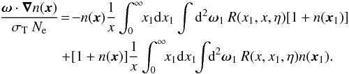 (A.8)For
the plane-parallel atmosphere, this reduces to
(A.8)For
the plane-parallel atmosphere, this reduces to 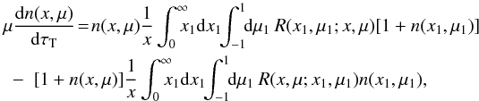 (A.9)where
dτT = − σTNeds = κe dm,
μ and μ1 are the cosines of the angle
relative to the normal,
(A.9)where
dτT = − σTNeds = κe dm,
μ and μ1 are the cosines of the angle
relative to the normal, 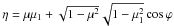 and
and
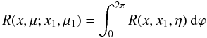 (A.10)is the
azimuth-integrated RF. Rewriting Eq. (A.9) in terms of the intensity I(x,μ), we
get the radiative transfer Eq. (10)
that accounts for electron scattering with the scattering opacity and the source
function given by Eqs. (12) and (14), respectively.
(A.10)is the
azimuth-integrated RF. Rewriting Eq. (A.9) in terms of the intensity I(x,μ), we
get the radiative transfer Eq. (10)
that accounts for electron scattering with the scattering opacity and the source
function given by Eqs. (12) and (14), respectively.
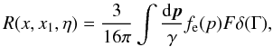
A.2. Redistribution functions
The expression (A.5) for the RF can
be simplified by taking the integral over p with the
help of the three-dimensional delta-function and using the identity

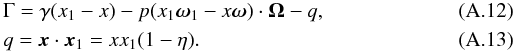
 (A.11)where we have
dropped the subscript 1 from the electron quantities and
(A.11)where we have
dropped the subscript 1 from the electron quantities and
 \arraycolsep1.75ptTo
integrate over angles in Eq. (A.11),
we follow the recipe proposed by Aharonian &
Atoyan (1981) (see also Prasad et al.
1986; Poutanen & Vurm 2010),
choosing the polar axis along the direction of the transferred momentum
\arraycolsep1.75ptTo
integrate over angles in Eq. (A.11),
we follow the recipe proposed by Aharonian &
Atoyan (1981) (see also Prasad et al.
1986; Poutanen & Vurm 2010),
choosing the polar axis along the direction of the transferred momentum
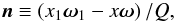 (A.14)where
 (A.15)Thus, the integration
variables become
cosα = n·Ω
and the azimuth Φ. The RF (A.11) can
then be written as
(A.15)Thus, the integration
variables become
cosα = n·Ω
and the azimuth Φ. The RF (A.11) can
then be written as 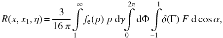 (A.16)where now
 (A.17)Integrating over
cosα using the delta-function, we get
(A.17)Integrating over
cosα using the delta-function, we get 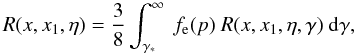 (A.18)where the
integration over the electron distribution can been done numerically. Here we
introduce the RF for monoenergetic electrons
(A.18)where the
integration over the electron distribution can been done numerically. Here we
introduce the RF for monoenergetic electrons 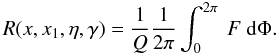 (A.19)We need to
substitute
(A.19)We need to
substitute 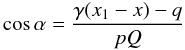 (A.20)into
the expression for F. The condition |cosα| ≤ 1
provides the constraint
(A.20)into
the expression for F. The condition |cosα| ≤ 1
provides the constraint  (A.21)Integrating
over azimuth Φ in Eq. (A.19) gives the
exact analytical expression for the RF that is valid for any photon and electron
energy (Aharonian & Atoyan 1981; Nagirner & Poutanen 1994; Poutanen & Vurm 2010), which we use in our
calculations
(A.21)Integrating
over azimuth Φ in Eq. (A.19) gives the
exact analytical expression for the RF that is valid for any photon and electron
energy (Aharonian & Atoyan 1981; Nagirner & Poutanen 1994; Poutanen & Vurm 2010), which we use in our
calculations 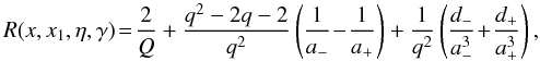 (A.22)where
 (A.23)We
note that the RF (A.19) satisfies the
detailed balance condition (Nagirner &
Poutanen 1994)
(A.23)We
note that the RF (A.19) satisfies the
detailed balance condition (Nagirner &
Poutanen 1994)  (A.24)The RF (A.11) is related to the scattering
kernel (8.13) of Pomraning (1973) as
R(x,x1,η) = σs(x1 → x,η)x1/x.
The form given by Eq. (A.16) is
equivalent to Eq. (A.4) of Buchler & Yueh
(1976). The derived RF for monoenergetic electrons (A.22) is equivalent to Eq. (A.5) of Buchler & Yueh (1976) and Eq. (14) of Aharonian & Atoyan (1981).
(A.24)The RF (A.11) is related to the scattering
kernel (8.13) of Pomraning (1973) as
R(x,x1,η) = σs(x1 → x,η)x1/x.
The form given by Eq. (A.16) is
equivalent to Eq. (A.4) of Buchler & Yueh
(1976). The derived RF for monoenergetic electrons (A.22) is equivalent to Eq. (A.5) of Buchler & Yueh (1976) and Eq. (14) of Aharonian & Atoyan (1981).
A very simple approximate expression for the RF can be obtained by assuming that the
scattering in the electron rest frame proceeds in the Thomson regime (i.e. coherent)
and is isotropic. This is equivalent to substituting F
by 4/3 in Eq. (A.19). We then get (Arutyunyan &
Nikogosyan 1980; Poutanen 1994; Poutanen & Svensson 1996) 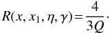 (A.25)Integrating
it over the Maxwellian distribution (A.6) gives
(A.25)Integrating
it over the Maxwellian distribution (A.6) gives  (A.26)This
approximate RF is also used in the calculations. We note that this RF also satisfies
the detailed balance condition (A.7).
(A.26)This
approximate RF is also used in the calculations. We note that this RF also satisfies
the detailed balance condition (A.7).
Appendix B: Method for solving the radiation transfer equation
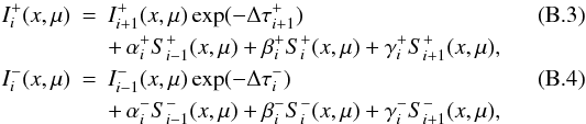
The formal solution of the radiative transfer equation gives a relation between the
outward I + (x,μ) and the inward
I−(x,μ) = I(x, − μ)
intensities at some depth point i (on the optical depth
grid  )
with the adjacent intensities
)
with the adjacent intensities 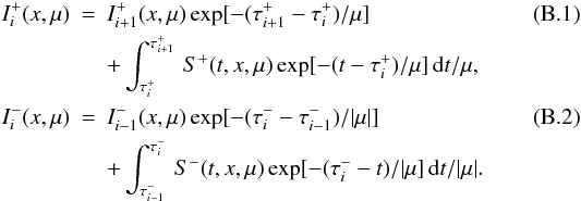 The
integrals can be replaced by the sums using the parabolic approximation
The
integrals can be replaced by the sums using the parabolic approximation
 where
where
 (B.5)\arraycolsep1.75ptand
 (B.6)At
the first depth point, the coefficients are
(B.6)At
the first depth point, the coefficients are
 (B.7)and at the last
point they are
(B.7)and at the last
point they are  (B.8)We note that the
inward and the outward opacities along the same ray are different (see Eq. (12)).
(B.8)We note that the
inward and the outward opacities along the same ray are different (see Eq. (12)).
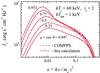 |
Fig. B.1
Comparison of the emergent spectra from a hot electron slab back-irradiated by a blackbody computed using the compps code and the code presented here. |
| Open with DEXTER | |
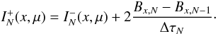
The formal solution for a given source function starts for the inward intensities from
the outer boundary condition (the lack of incoming radiation at the surface)
 (B.9)up to the last depth
point N. The intensities at the innermost depth point are found using
the inner boundary condition, which is taken from the diffusion approximation
(B.9)up to the last depth
point N. The intensities at the innermost depth point are found using
the inner boundary condition, which is taken from the diffusion approximation
 (B.10)The full solution is
found iteratively using an accelerated Λ-iteration. At the first iteration, the thermal
part of the source function is taken. For the subsequent iteration n,
the intensities obtained from the previous iteration n − 1 are used to
compute the current source functions
(B.10)The full solution is
found iteratively using an accelerated Λ-iteration. At the first iteration, the thermal
part of the source function is taken. For the subsequent iteration n,
the intensities obtained from the previous iteration n − 1 are used to
compute the current source functions  .
Iterations are continued until the relative change becomes smaller than the
predetermined accuracy
.
Iterations are continued until the relative change becomes smaller than the
predetermined accuracy 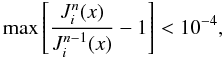 (B.11)where
Ji(x) are the mean
intensities. This solution method of the radiation transfer equation was tested for a
rather optically thin (Thomson optical depth τT = 2) and hot
(kTe = 60 keV) electron slab
back-illuminated by soft blackbody photons of
kTBB = 1 keV. The solution for the
emergent intensities obtained at five angles using our method were compared with the
solution obtained with the Comptonization code compps (Poutanen & Svensson 1996, see Fig. B.1).
(B.11)where
Ji(x) are the mean
intensities. This solution method of the radiation transfer equation was tested for a
rather optically thin (Thomson optical depth τT = 2) and hot
(kTe = 60 keV) electron slab
back-illuminated by soft blackbody photons of
kTBB = 1 keV. The solution for the
emergent intensities obtained at five angles using our method were compared with the
solution obtained with the Comptonization code compps (Poutanen & Svensson 1996, see Fig. B.1).
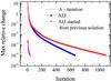 |
Fig. B.2
The maximum relative change in the solution of the radiation transfer equation at the final temperature correction computed by different versions of the accelerated Λ-iteration. |
| Open with DEXTER | |
In the optically thick case (τT ≫ 1), which is typical of
NS atmospheres, the convergence of the solution can be accelerated using the following
procedure. The difference between the formal solution obtained in the current
iteration I ± ,n,FS and the solution at
iteration n − 1 is increased by some factor
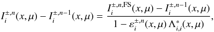 (B.12)where
 (B.13)and
 is the diagonal term of the
approximate Λ-operator
is the diagonal term of the
approximate Λ-operator  (B.14)The
acceleration is not high (about 30–40%) and the number of necessary iterations is still
large (see Fig. B.2). However, in the process of
the model atmosphere computation it is possible to use the source function from the
previous temperature iteration as the starting approximation for the current source
function (see details in Sect. 2). In this case,
the acceleration depends on the value of the temperature
corrections ΔTi. At the first few
temperature iterations, when ΔTi are large,
the acceleration is insignificant, but at later iterations, when
ΔTi are relatively small,
the accelerated Λ-iterations converge very quickly (Fig. B.2).
(B.14)The
acceleration is not high (about 30–40%) and the number of necessary iterations is still
large (see Fig. B.2). However, in the process of
the model atmosphere computation it is possible to use the source function from the
previous temperature iteration as the starting approximation for the current source
function (see details in Sect. 2). In this case,
the acceleration depends on the value of the temperature
corrections ΔTi. At the first few
temperature iterations, when ΔTi are large,
the acceleration is insignificant, but at later iterations, when
ΔTi are relatively small,
the accelerated Λ-iterations converge very quickly (Fig. B.2).
Appendix C: Comparison with Madej’s code
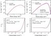 |
Fig. C.1
Left panels: comparison of emergent spectra and temperature structures of the models computed by our code (solid curves) and Madej’s code (dashed curves), when electron scattering is approximated by coherent Thomson scattering. Right panels: same as left, but when the exact RF was used to compute Compton scattering. The spectrum computed by us using the Madej’s temperature structure is shown by the dotted curve and the spectrum computed with a relative accuracy of 10-2 is presented by dash-dots. |
| Open with DEXTER | |
The only other attempt to compute NS atmospheres using an integral approach to Compton scattering going beyond the Kompaneets approximation was that of J. Madej et al. (Madej 1991; Madej et al. 2004; Majczyna et al. 2005). They used an angle-averaged RF for Compton scattering derived by Guilbert (1981). It is important to compare our results with those obtained by Madej’s code for the same input parameters. We selected our fiducial model as a testbed and computed two models. In the first, we approximated electron scattering by coherent Thomson scattering. In the second, the exact fully relativistic RF for Compton scattering was used. Calculations for identical parameters were performed with Madej’s code (J. Madej & A. Różańska, priv. comm.). A comparison between the results is shown in Fig. C.1.
We see that the Thomson scattering models are very close to each other, in terms of both the spectra and the temperature structures (Fig. C.1, left panels). However, the models with Compton scattering differ substantially (Fig. C.1, right panels). Temperatures in the upper layers with column densities less than 103 g cm-2 are lower in our model by up to 5−15%, and our spectrum (solid curve) is much more peaked and softer than that computed by Madej’s code (dashed curve). We also note that our spectrum is very close to the diluted blackbody spectra, which cannot be said about Madej’s spectrum.
We can suggest two hypotheses to explain the discrepancies. First, there is a difference in the RF used by the two codes. We employed the exact relativistic RF (see Appendix A.2), which had been extensively studied and tested against Monte-Carlo simulations (Stern et al. 1995; Zdziarski et al. 2000). Madej and collaborators (Madej 1991; Madej et al. 2004; Majczyna et al. 2005) used the (angle-averaged) RF derived by Guilbert (1981) (see his Eqs. (8) and (10)), which differs from the correct expression (A.19) by an additional factor [1 − (β·n)(n·ω1)] /(1 − β·ω1), which appeared from an error in the Jacobian. Guilbert’s RF also does not satisfy the detailed balance condition (A.24) and therefore the RF integrated over the electron distribution does not satisfy the condition (A.7) either. Because the energy transfer by Compton scattering scales as β2, the error on the order of β obviously invalidates all the results obtained with this RF.
Second, some of the discrepancies could be connected to a difference in the computation of the radiation transfer and the atmosphere modeling. We illustrate this in Fig. C.1 (top right panel). Using our radiation transfer code, we computed the spectrum using the temperature structure from Madej’s calculations. When calculations proceeded until the accuracy of 10-4 was reached (dotted curve), the spectrum was much above our benchmark spectrum, i.e. it had a much higher effective (and color) temperature. If calculations were stopped at a lower accuracy of 10-2 (dash-dotted curve), the spectrum was found to be similar to Madej’s spectrum. This suggests that the radiation transfer iterations with Madej’s code did not sufficiently converge.
Madej et al. use the partial linearization method described in Mihalas (1978, p. 179) and modified to include Compton scattering. Their radiation transfer equation is rewritten to include the linearized part of the radiative equilibrium equation. The solution of this generalized radiation transfer equation satisfies simultaneously the radiative equilibrium to the first order. Using the computed radiation field, the temperature correction for the current temperature structure of the atmosphere is found. This procedure is iterated until some convergence criterion is satisfied, for example, the emergent bolometric flux is accurate to within 0.1%. In this method, the accuracy of the current solution of the radiation transfer equation is on the order ΔT/T, which is about 10-2−10-3 at the last iteration. We have shown above that this internal accuracy is insufficient to obtain the exact solution of the radiation transfer equation when Compton scattering is taken into account. We note that using this method is not possible to solve the radiation transfer equation for a given atmosphere model or, for example, for a homogeneous isothermal slab. This means that it cannot be checked independently of the atmosphere modeling.
Appendix D: Atmosphere model spectra and color-corrections
Table D.1 gives the color-correction and dilution factors from the blackbody fits to 484 atmosphere model spectra (fluxes), which in their turn are given in Table D.2. Table D.3 contains the emergent specific intensities at three angles. Tables D.1−D.3 are only available in electronic form at the CDS. The Xspec code utilizing the models is available from the authors on request.
© ESO, 2012
Current usage metrics show cumulative count of Article Views (full-text article views including HTML views, PDF and ePub downloads, according to the available data) and Abstracts Views on Vision4Press platform.
Data correspond to usage on the plateform after 2015. The current usage metrics is available 48-96 hours after online publication and is updated daily on week days.
Initial download of the metrics may take a while.