| Issue |
A&A
Volume 531, July 2011
|
|
|---|---|---|
| Article Number | L1 | |
| Number of page(s) | 6 | |
| Section | Letters | |
| DOI | https://doi.org/10.1051/0004-6361/201116975 | |
| Published online | 30 May 2011 | |
Online material
Appendix A: Gauss fit of data
The data are fitted by Gaussians, with the exception of the narrow absorption component. Figure A.1 shows the example of the H2O 111–000 line, with the residual plotted below. Furthermore, Fig. A.1 shows the CO 3–2 line scaled and overplotted on the H2O 111–000 line, highlighting the similar line profile in the EHV components.
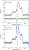 |
Fig. A.1
Top: Gauss fit of the H2O 111–000 line (red) with the residual shown below (offset at − 0.1 K). The central absorption feature is not fitted. Bottom: CO 3–2 scaled to the peak intensity of H2O in the bullets and overplotted on the H2O 111–000 line. |
| Open with DEXTER | |
Appendix B: RADEX results
The non-LTE, escape-probability code RADEX was used to create rotational diagrams for H2O and CO in the optically thin limit. Collisional rate coefficients are from Faure et al. (2007) and Yang et al. (2010), respectively. The same transitions as observed were then used to calculate the rotational temperature as function of Tkin and nH. The results are shown in Fig. B.1.
RADEX was also used to calculate the optical depth, τ of the H O 110–101 line at 557 GHz. Results are shown in Fig. B.2, where also the beam-filling factor is shown as a function of H2O column density for the three different models.
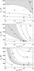 |
Fig. B.1
Trot of optically thin H2O emission (top), optically thick H2O emission (N = 1017 cm-2; middle) and optically thin CO emission (bottom) determined from RADEX simulations. Trot is calculated from the same transitions as in Sect. 2, i.e., excluding the ground-state transitions. The gray area indicates the observed values of Trot. The points indicate the different physical conditions examined; model 1 (red) has (T, n) = (150 K, 106 cm-3) for the EHV components and (100 K, 106 cm-3) for the broad component. Model 2 (blue) has (T, n) = (500 K, 105 cm-3) for the EHV components, respectively. Model 3 (green) has (T, n) = (500 K, 106 cm-3) for all components. |
| Open with DEXTER | |
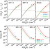 |
Fig. B.2
Top: τ of the H |
| Open with DEXTER | |


© ESO, 2011
Current usage metrics show cumulative count of Article Views (full-text article views including HTML views, PDF and ePub downloads, according to the available data) and Abstracts Views on Vision4Press platform.
Data correspond to usage on the plateform after 2015. The current usage metrics is available 48-96 hours after online publication and is updated daily on week days.
Initial download of the metrics may take a while.