| Issue |
A&A
Volume 531, July 2011
|
|
|---|---|---|
| Article Number | A91 | |
| Number of page(s) | 17 | |
| Section | The Sun | |
| DOI | https://doi.org/10.1051/0004-6361/201016006 | |
| Published online | 20 June 2011 | |
Online material
Appendix A: Neutron monitor stations
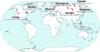 |
Fig. A.1
Stations that provided the neutron monitor data. Cutoff rigidity (Rc), latitude, and longitude are written under the name of the station. |
| Open with DEXTER | |
A grid of ground level cosmic ray detectors, located in a number of stations around the globe, including both high-energy muon detectors and lower energy neutron monitors, cover different geographic latitudes and longitudes. This is important for cosmic ray research owing to the interaction of cosmic rays (i.e. protons, which make up 90% of the incoming cosmic rays) with geomagnetic field. The effects of this interaction is given through vertical geomagnetic cutoff rigidity, i.e. the lowest, latitude-dependent rigidity, associated with a particle penetrating the Earth‘s magnetic field (particles of lower rigidity do not enter the atmosphere). Rigidity (R = pc/|q|,where p and q are particle impulse and charge, and c is speed of light) is dependent on both particle energy and the magnetic field in question, representing the influence of the magnetic field on the trajectory of the particle. Thus, a particle of the energy of 1 GeV will be detected near the pole, where the cutoff rigidity is very low, but not near the equator, where only high-energy particles can penetrate the geomagnetic field deep enough for the secondaries to reach the detector. Consequently, this will influence the CR flux, as detected by the ground-based monitors, since the flux will evidently be larger at higher latitudes (i.e. for smaller cutoff rigidities). Figure A.1 shows the location of neutron monitor stations used in our research, along with the associated cutoff rigidity.
Appendix B: List of events
Notes on Tables B.1 and B.2: The event date was determined by the onset of Forbush decrease. Dashes stand for missing data, whereas question marks are attributed to measurements that are unclear. Events associated with shock are denoted with “Y”, those not associated with shock are denoted N. The phenomenon where CR count in the recovery phase of Forbush decrease reaches higher values than the ones in the pre-decrease phase is referred to as over-recovery. It was determined only in measurements I and categorized as follows:
-
“N” – events that show no over-recovery and are not interrupted by another event;
-
“N*” – events that show no over-recovery, but are interrupted by another event;
-
“Y*” – events that show over-recovery, but start in the recovery phase of another event;
-
“Y” – events that show over-recovery and do not start in the recovery phase of another event.
Measurements I.
Measurements II.
Appendix C: Random sample analysis
In order to also check the reliability of the analysis performed by two independent people, denoted as measurements I and II, random subsamples of events from both measurements were generated. Each subsample consisted of 50 events, where one half was taken randomly from measurement I and another half from measurement II. The correlation coefficient was then calculated for each random subsample, and the procedure was repeated one million times. This provided the distribution of correlation coefficients as shown in Fig. C.1. This also allowed identifying outliers, as they led to a double-peaked distribution, as can be seen in the δB(| FD|) and tFD(tB) data in Figs. C.2 and C.3.
The median values of the distributions of correlation coefficients shown in Fig. C.1 correspond approximately to values obtained by the linear regression analysis of measurements I and II (see Tables 2 and 4 in Sects. 3.2 and 3.4). The situation is somewhat different for the examples in Figs. C.2a and C.3a due to double-peaked distributions. Removal of the outliers (29 october 2003 and 8 June 2000 in Figs. C.2b and C.3b, respectively) results in a quite regular distribution (see Figs. C.2b and C.3b), characterized by somewhat smaller median of correlation coefficients, which match the values obtained by the linear regression analysis of measurements I and II, when the outliers are removed (r = 0.61 for δB(|FD|) in measurements I, r = 0.66 for δB(| FD|) in measurements II and r = 0.54 for tFD(tB) in measurements II). It should be noted that the outlier in tFD(tB) data is only present in measurements II data and is therefore a source of the difference in the correlation coefficients for the two samples (see Table 3).
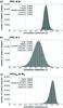 |
Fig. C.1
Correlation histogram for a) FD magnitude, |FD|, versus IMF magnitude, B; b) |FD| versus solar wind speed, vrel; c) the product of the FD magnitude and duration, |FD|tFD, versus the product of the magnetic field enhancement and duration, BtB. The y-axis represents the number of correlations in specific correlation coefficient class (x-axis). Each histogram is based on one million calculated correlation coefficients. |
| Open with DEXTER | |
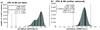 |
Fig. C.2
Correlation histograms for FD duration, tFD, versus the disturbance duration, tB. a) All events used to generate the samples; b) the event identified as an outlier (29.10.2003.) was removed from the analysis. The y-axis represents the number of correlations in specific correlation coefficient class (x-axis). Each histogram is based on one million calculated correlation coefficients. |
| Open with DEXTER | |
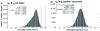 |
Fig. C.3
Correlation histograms for FD magnitude, |FD|, versus IMF fluctuations enhancement, δB. a) All events used to generate the samples; b) event identified as an outlier (08.06.2000.) was removed from the analysis. The y-axis represents the number of correlations in specific correlation coefficient class (x-axis). Each histogram is based on one million calculated correlation coefficients. |
| Open with DEXTER | |
© ESO, 2011
Current usage metrics show cumulative count of Article Views (full-text article views including HTML views, PDF and ePub downloads, according to the available data) and Abstracts Views on Vision4Press platform.
Data correspond to usage on the plateform after 2015. The current usage metrics is available 48-96 hours after online publication and is updated daily on week days.
Initial download of the metrics may take a while.