| Issue |
A&A
Volume 529, May 2011
|
|
|---|---|---|
| Article Number | A129 | |
| Number of page(s) | 19 | |
| Section | Stellar atmospheres | |
| DOI | https://doi.org/10.1051/0004-6361/201016272 | |
| Published online | 18 April 2011 | |
Online material
Appendix A: Details of the atmospheric models
A.1. General remarks
The two aspects discussed in this paper – pulsation of the stellar interior and the formation of a dusty stellar wind – have a considerable influence on the outer layers of an AGB star and hydrostatic model atmospheres are, therefore, often not an adequate approach to describe the resulting complex stratifications and dynamic effects. As a consequence, dynamic model atmospheres were developed to simulate mass-losing LPVs (Sect. 1).
The majority of the AGB stars found are of spectral type M (e.g., Nowotny et al. 2003; Battinelli et al. 2003; Rowe et al. 2005) and have oxygen-rich14 atmospheric chemistries with C/O < 1. This is also reflected in the mineralogical species constituting the dust grains that occur in the winds. Observational spectroscopic studies revealed a rich mineralogy in the dusty outflows of M-type giants (e.g., Molster & Waters 2003, and references therein). However, the dust formation process in the atmospheres of such objects is so far not fully understood (cf. Höfner 2009) and the open question concerning the driving mechanism for the wind in the O-rich case is not solved, yet (Woitke 2006, 2007; Höfner 2007). One possibility to drive a wind was sketched by Höfner (2008) with the help of big ( ≈ μm) Fe-free silicate grains (i.e., Forsterite Mg2SiO4) and their substantial radiative scattering cross section.
As a star evolves during the AGB phase, a combination of nucleosynthesis and convection processes can lead to a drastic change of the chemical composition of the outer layers (e.g., Busso et al. 1999; Herwig 2005). Having been converted to a carbon star (Wallerstein & Knapp 1998) with an atmospheric chemistry characterised by C/O > 1, the spectrum of this star is strongly changed and shows prominent features of C-bearing molecules (Paper I, Fig. 3). This transformation to spectral type C is, in addition, highly relevant for the circumstellar dust chemistry which is believed to be simpler than the corresponding one of M-type stars. Apart from the few dust species identifiable via their characteristic emission features, as for example SiC or MgS (see Molster & Waters 2003), the majority of the formed dust grains are composed of amorphous carbon (amC). Although they are not recognisable in the spectra by a distinctive spectral feature because of the featureless extinction properties (e.g., Fig. 3 or Andersen et al. 1999), amorphous carbon dust plays a crucial role for driving stellar winds via radiation pressure as outlined for example in NHA10. Moreover, the formation and evolution of amC grains can be treated in a consistent way (Gail & Sedlmayr 1988; Gauger et al. 1990) in numerical models. This enables us to calculate detailed and self-consistent models for the atmospheres of pulsating red giants including the developing winds.
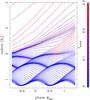 |
Fig. A.1
Movement of mass shells with time at different depths of model S, depicting a pulsation-enhanced dust-driven wind. The shown trajectories follow the evolution with time of certain matter elements starting from the distribution of adaptive grid points (higher density of points at the locations of shocks) at an arbitrarily chosen point in time (in this case at the end of the plotted sequence). Colour-coded is the degree of condensation of the available carbon into amorphous carbon dust grains. |
| Open with DEXTER | |
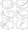 |
Fig. A.2
Characteristic properties of model S. Plotted in panel a) is the bolometric lightcurve resulting from the variable inner boundary (piston), the circles mark instances of time for which snapshots of the atmospheric structure were stored by the radiation-hydrodynamics code, partly labelled with the corresponding values for phase φbol. The dotted vertical lines mark the points in time of φbol = 0.0 and 1.0, respectively, while the horizontal line marks L ⋆ of the initial model which is almost equal to ⟨ L ⟩ of the dynamical calculation (NHA10). The other panels show the atmospheric structures of the initial hydrostatic model (thick black line) together with selected phases φbol of the dynamic calculation during one pulsation cycle (colour-coded in the same way as the phase labels of panel a)). While panel b) shows the classical plot of gas temperature vs. gas pressure used to characterise stellar atmospheres, the middle and lower panels illustrate the radial structures of gas temperatures c), gas densities d), gas velocities e), and condensation degrees of the element carbon into amorphous carbon dust grains f). |
| Open with DEXTER | |
A.2. Dynamic model atmospheres
For the synthetic photometry presented in this work we used the dynamic model atmospheres presented in Höfner et al. (2003). These models simulate pulsation-enhanced dust-driven winds (caused by radiation pressure on amorphous carbon dust particles), which is the most widely accepted scenario for mass loss on the AGB in the C-rich case. They are well suited to describe the complex behaviour of all atmospheric layers – from the inner photosphere out to the cool wind region – of pulsating AGB variables with intermediate to high mass-loss rates15. This is accomplished by a combined and self-consistent solution of hydrodynamics, frequency-dependent radiative transfer and a detailed time-dependent treatment of dust formation and evolution (for details see Höfner et al. 2003). Additional descriptions of the dynamical models can be found in Gautschy-Loidl et al. (2004), Nowotny (2005), Nowotny et al. (2005a, 2010), and Mattsson et al. (2007, 2010).
In a recent study, Mattsson et al. (2010) computed a grid of C-rich dynamic model atmospheres and investigated the resulting mass loss properties (e.g., mass-loss rates Ṁ, wind terminal velocities u∞, dust condensation degrees in the outflows fc) as a function of stellar and piston parameters. Here we made use of only one selected atmospheric model, the parameters of which are listed in Table 1. This model S is representative of a typical C-type Mira with intermediate mass loss and was successful in the past in simulating observational results as diverse as low-resolution spectra (Gautschy-Loidl et al. 2004), line profile variations (Nowotny et al. 2005a, 2005b, 2010) and interferometric properties (Paladini et al. 2009).
In Fig. A.1 the motions of layers at different atmospheric depths for the chosen model are illustrated, while the corresponding atmospheric structures are shown in Fig. A.2. The dynamic calculation starts with a hydrostatic initial model characterised by stellar parameters as given in the first part of Table 1. This comparably compact and dust-free atmosphere is constructed in a similar way as classical hydrostatic model atmospheres for red giants, especially the COMARCS models used in Paper I (for a quantitative comparison see Appendix A.3). The effects of stellar pulsation are subsequently introduced by a variable inner boundary, representing a sinusoidally moving piston at the innermost radial point of the model with parameters as listed also in Table 1. Apart from the kinetic energy input, this also prescribes a changing luminosity input at the inner boundary (Fig. A.2a), for a detailed description we refer to Eqs. (1) and (2) in NHA10 as well as the corresponding explanations there. A shock wave triggered by the pulsation emerges during every pulsation cycle and propagates outwards through the atmosphere causing a levitation of the outer layers. In the wake of the shocks (post-shock regions) the physical conditions – strongly enhanced densities at temperatures low enough to allow for dust condensation – provide the necessary basis for the formation of amC grains (e.g., Sedlmayr 1994). Radiation pressure acting upon the formed dust particles results in an outwards directed acceleration. Subsequent momentum transfer between the grains and surrounding gas via direct collisions (e.g., Sandin & Höfner 2004) leads to the development of a stellar wind. The temporally varying radial structure of the dynamic model atmosphere (Fig. A.2) deviates significantly from the hydrostatic case. Not resembling the intital model at any point in time, the atmospheric structure of the fully developed mass-losing model becomes extremely extended in comparison, with strong local variations superposed on the shallow density gradient.
A.3. Comparison of hydrostatic initial models and COMARCS models
In the course of our synthetic photometry we tested how similar the hydrostatic intial models of the dynamical calculations (cf. Appendix A.2) are compared with classical hydrostatic model atmospheres like the ones used in Paper I. For the parameters of the initial model of model S (Table 1) no converging solution could be otained with the MARCS code for numerical reasons. Therefore, we turned to the slightly more moderate model M used in Nowotny et al. (2010) for line profile modelling. The stellar parameters of the corresponding initial model are compared to the parameters of our closest COMARCS model in Table A.1. Note that there are marginal differences as the primary input parameters are not the same for the code to compute initial models and the MARCS code. The structures of the two atmospheric models are compared in Fig. A.3. Apart from the larger range covered by the COMARCS model, the radial structures are very similar for most of the depth points. This is also reflected in the resulting spectra which are shown in Fig. A.3, too. To quantify the differences for the different types of hydrostatic models we also compared the synthetic photometry in the chosen set of broad-band filters (Sect. 2.3). The results, as listed in Table A.2, show that the deviations are quite low. This is especially valid in the NIR. Thus, we conclude that the initial models – which are constructed using fewer frequency points and no convection description compared to the COMARCS models of Paper I – are comparable to other hydrostatic atmospheric models. They represent adequate starting points for the subsequent dynamical calculations, where the effects of pulsation and stellar winds lead to considerable changes in the radial structures (Fig. A.2).
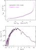 |
Fig. A.3
Comparison of the atmospheric structures of the models in Table A.1 (upper panel) and the resulting low-resolution spectra based on these (lower panel). |
| Open with DEXTER | |
Appendix B: Looping the colour
A certain disagreement was found in Sect. 4.3 between the modelling results and corresponding observational data. In Fig. 13 one recognises that the model loops counter-clockwise through the colour − colour plane, while the average variation of RU Vir in Fig. 14 (dashed line) passes clockwise through an ellipse in this CCD. It can be shown by a simple test that such a change in the sense of the rotation can easily be introduced by a change of sign in the phase shift between lightcurves in different filters, which may itself be linked to the dust description in the modelling context, cf. Sect. 4.2.
To illustrate this, we used the simulated JHK lightcurves from Fig. 8 and applied artificial phase shifts of Δφ = ± 0.1 such that the phases of light maximum in the different filters occur at increasing or decreasing phases φv. The resulting light variations are shown in the upper panel of Fig. B.1.
Based on these lightcurves, we computed colour indices which are shown in the lower panel of the figure. For the JHK variations in phase (black), the object moves along a straight line from bluer to redder colours in the CCD. The ranges in (J − H) and (H − K) are determined by the amplitude differences of the individual lightcurves. If the above mentioned artificial phase shift is applied to the JHK lightcurves (red, green), the star follows a loop through the CCD which covers a larger range in both colour indices. In addition, Fig. B.1 demonstrates that the sense of rotation changes when the sign of the phase shift Δφ is inverted.
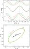 |
Fig. B.1
Upper panel: simulated JHK lightcurves adopted from Fig. 8 (sinusoidal fits to the observational data there) with artificial phase shifts of Δφ = −0.1/0/+0.1 (red, black, and green lines, respectively) imposed in all three filters. Lower panel: resulting variations in an NIR colour − colour diagram, colour coded correspondingly. The labels mark locations occupied by the object at certain phases φv, while the arrows designate the sense of rotation of the loops. |
| Open with DEXTER | |
© ESO, 2011
Current usage metrics show cumulative count of Article Views (full-text article views including HTML views, PDF and ePub downloads, according to the available data) and Abstracts Views on Vision4Press platform.
Data correspond to usage on the plateform after 2015. The current usage metrics is available 48-96 hours after online publication and is updated daily on week days.
Initial download of the metrics may take a while.