| Issue |
A&A
Volume 522, November 2010
|
|
|---|---|---|
| Article Number | A91 | |
| Number of page(s) | 19 | |
| Section | Interstellar and circumstellar matter | |
| DOI | https://doi.org/10.1051/0004-6361/201015158 | |
| Published online | 05 November 2010 | |
Online material
Appendix A: A survey of EHV SO emission in I04166
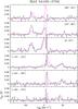 |
Fig. A.1
SO(32 − 21) (black) and CO(2 − 1) (red) spectra along the central axis of the I04166 outflow. The CO spectra have been scaled down by a factor of 20, and the offsets are referred to the IRAS nominal position (α(J2000) = 4h19m42ṣ6, δ(J2000) = +27°13′38′′). |
| Open with DEXTER | |
The detection of relatively strong SO emission in the EHV component of both L1448 and I04166 target positions was unexpected. No SO emission from EHV gas had previously been reported, so no information on its distribution and relation to other EHV tracers like CO and SiO was available. To better characterize this SO emission, we made small maps around both sources. In I04166, we observed 6 positions along the outflow axis and in L1448 we observed three positions. This appendix presents the I04166 data (the more limited L1448 survey is consistent with the I04166 results).
Figure A.1 shows the SO(32 − 21) and CO(2 − 1) spectra observed simultaneously along the I04166 outflow axis. As can be seen, EHV SO emission was detected in at least 5 of the 6 target positions, both towards the red and blue lobes. Considering the limited S / N of the data and the different beam size of the two transitions (24′′ in SO(32 − 21) and 11′′ in CO(2 − 1)), we find a good match between the SO and CO data, indicating that the two EHV emissions originate from the same gas. In this respect, we can consider the position selected for the molecular survey as a likely representative of the outflow as a whole.
To further characterize the EHV SO emission in the I04166 outflow, we study the ratio between the CO(2 − 1) and SO(32 − 21) integrated intensities. Table A.1 presents the values measured in our survey using the LSR velocity ranges −43 to −26 km s-1 for the blue EHV gas and 37 to 54 km s-1 for the red EHV gas. As can be seen, the CO(2 − 1)/SO(32 − 21) ratio in the innermost 4 positions is on the order of 20, which is consistent with the value derived in the molecular survey of Sect. 3. In the outermost position of each outflow lobe, however, the SO(32 − 21) emission weakens significantly, and the CO(2 − 1)/SO(32 − 21) ratio increases to about 40 towards the northern (blue) lobe and twice as much towards the southern (red) lobe.
The close to constant CO/SO intensity ratio along the inner EHV jet suggests that both the SO excitation and the abundance relative to CO are close to constant for this outflow component over the central ≈ 0.03 pc, and that they have values similar to those derived for the (8′′, 14′′) position, for which additional transitions of both species were observed. The increase of the CO/SO intensity ratio in the outer outflow, on the other hand, suggests that there is a drop in the SO abundance or excitation of the EHV gas about 0.05 pc from the outflow source. Lacking additional SO data, we use the CO and SiO observations of Santiago-García et al. (2009) to investigate this drop. The high-resolution CO and SiO interferometric observations showed a similar factor of 2-3 increase in the CO(2 − 1)/SiO(2 − 1) ratio in the EHV component as a function of distance from the protostar. The interferometric data, in addition, showed that both the CO and SiO emitting regions broaden with distance to the YSO, suggesting that the EHV gas is spreading laterally as it moves away from the protostar (in agreement with models of internal working surfaces, Dutrey et al. 1997; Santiago-García et al. 2009). In this case, it seems therefore likely that the excitation of SiO drops faster than that of CO due to its higher dipole moment, and that the observed change in the CO/SiO ratio is at least in part produced by a change in excitation. As the SO molecule has also a high dipole moment, it is very likely that the increase in the CO/SO ratio with distance from I04166 also results, at least in part, from a change in excitation. Multitransition observations are required to fully constrain the characteristics of the EHV gas in I04166.
Although our observations seem to represent the first detection of SO in EHV gas, bright SO emission in the jet-like components of the HH211 and Ori-S6 outflows have been recently reported by Lee et al. (2010) and Zapata et al. (2010), respectively. The jet-like component of these outflows has significantly lower velocity than the components in L1448 and I04166, and their emission does not form distinct EHV features in the CO spectra like those shown in Fig. 2. These jet-like components, however, may represent a similar phenomenon to the EHV gas, and may owe their low radial velocity just to a location close to the plane of the sky. Lacking accurate measurements of outflow inclination angles, a comparison between the chemical properties of these objects may help test the idea that all the jet-like components share a common physics (and likely origin). If so, chemical composition may result a more discriminant tracer of outflow properties than gas kinematics, and the presence of EHV gas in outflows may be more common among Class 0 sources than currently recognized.
Appendix B: Correction for differential beam dilution
The beam size of a diffraction-limited telescope like the IRAM 30 m depends linearly on the operating wavelength, so for a given molecule, transitions having different rest frequencies are observed using different angular resolutions. At the CO(1 − 0) frequency, for example, the FWHM of the 30 m main beam is about 21 arcsec, while the main beam size for CO(2 − 1) is half that value (Greve et al. 1998). This significant change in the beam size with frequency, together with the small angular size of the regions under study, makes each transition in our survey suffer from a different amount of beam dilution. Such a differential effect needs to be corrected before using the observed intensities to derive molecular abundances, or otherwise the high frequency (small beam) transitions will be over weighted, producing an overestimate of both the molecular excitation and the species column density. In this appendix we present the method we have used to compensate for this common observational problem.
Properly correcting all our survey data for the effects of beam dilution would require making high angular resolution maps for each transition. In the absence of such data, we used observations of the main outflow tracer, CO, to characterize the distribution of gas in the vicinity of our survey targets, and to estimate how the observed spectrum depends on the beam size. To this end, we made a Nyquist-sampled map around each outflow target in CO(2 − 1), as this transition provides an effective angular resolution higher than most transitions in our survey ( ≈ 11′′). This CO(2 − 1) map was used to simulate observations with larger beam sizes by convolving the Nyquist-sampled spectra to the required resolution. As a result, we produced a grid of CO(2 − 1) spectra with effective beam sizes ranging from about 12′′ (close to the beam size for CO(2 − 1)) to about 30′′ (larger than the largest beam in our survey). To double check the I04166 results (where a pointing error was suspected in the Nyquist map), we repeated the calculation using the combined Plateau de Bure-30 m data set from Santiago-García et al. (2009), which contains all the spatial frequencies, is independent of our new 30 m Nyquist-sampled map, and has an angular resolution of about 3′′.
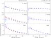 |
Fig. B.1 Variation of the CO(2 − 1) integrated
intensity as a function of total convolving beam size (normalized to the 16′′ value)
for the three outflow velocity regimes used in the molecular survey. The intensities
have been determined by convolving appropriately either IRAM 30 m Nyquist-sampled
maps (blue squares) or a combined Plateau de Bure interferometer+30 m data set (red
triangles). The dashed lines represent a set of fits with the form
|
| Open with DEXTER | |

The systematic dependence of the integrated intensity with observing beam size shown in
Fig. B.1 suggests that the effect of beam dilution
can be corrected, at least to first order, using a simple parameterization. For a
symmetric Gaussian beam, the beam dilution factor is proportional to
 if the source
is point like, to
if the source
is point like, to  if the
source one dimensional, and trivially equal to
if the
source one dimensional, and trivially equal to  if the source is infinitely
extended in two dimensions. It seems therefore reasonable that when fitting the curves of
Fig. B.1, we use an expression of the form
if the source is infinitely
extended in two dimensions. It seems therefore reasonable that when fitting the curves of
Fig. B.1, we use an expression of the form
 , where
α is a free parameter expected to lie between 0 and 2. This expectation
is confirmed by the data, and as the dashed curves in Fig. B.1 show, the analytic expression fits the data well inside the range of
observations. The α coefficient in the fit is 0.6, 0.75, and 0.9 for the
s-wing, f-wing, and EHV ranges of I04166, and 0.1, 0.3, and 1.0 for the same ranges in
L1448, respectively. Of particular interest is the close-to-1 values derived for the
EHV range in both outflows, a further indication that this fastest outflow regime is
highly collimated.
, where
α is a free parameter expected to lie between 0 and 2. This expectation
is confirmed by the data, and as the dashed curves in Fig. B.1 show, the analytic expression fits the data well inside the range of
observations. The α coefficient in the fit is 0.6, 0.75, and 0.9 for the
s-wing, f-wing, and EHV ranges of I04166, and 0.1, 0.3, and 1.0 for the same ranges in
L1448, respectively. Of particular interest is the close-to-1 values derived for the
EHV range in both outflows, a further indication that this fastest outflow regime is
highly collimated.
With the above fits we have
converted all measured integrated intensities into equivalent values for a 16′′ beam,
which is the average size of the beams used in in our survey. The excitation and column
density estimates presented in this paper therefore represent estimates of these
parameters inside a 16′′-diameter beam.
Appendix C: Fitting multiple-component spectra with templates
The spectra of HCN and CH3OH contain multiple components that partly overlap, and to calculate the integrated intensity of each of these components in each outflow regime, we need a method to disentangle them. An inspection of the data shows that in each multi-component spectrum, all components present similar shape and differ only in velocity and relative intensity, and this suggests that it should be possible to disentangle the outflow contributions by fitting the complex spectrum with a synthetic one made of multiple copies of the same line profile. To carry out such a fitting procedure, we have taken spectra from single lines (from CO, SO, CS, or SiO) as templates, made copies of them using the CLASS software, and shifted each template in frequency by the appropriate value for each component (as provided by the Cologne Database for Molecular Spectroscopy, see Müller et al. 2001, 2005). By varying the relative intensity of each template, which is the only free parameter in the procedure, we have fitted the multi-component spectra, and from this fit, we estimate the integrated intensity of each line component in the three outflow regimes (only the outflow part was fitted while the often optically thick ambient emission was ignored).
To identify the best fit solution, we selected a set of velocity ranges in the spectrum where the overlap between components is minor or where one component clearly dominates the emission, and we required that the synthetic spectrum matched the observed integrated intensity within the noise level. For the case of HCN(1 − 0), we found that the three hyperfine components had relative intensities very close to their statistical weights, suggesting that the outflow emission is optically thin and that the excitation of the sublevels is close to LTE. By fixing the relative intensities of the components to their statistical weights, the only one free parameter left to fit the observed emission profile was a global scaling factor.
As shown in Fig. 4, different species present slightly different outflow components, reflecting their peculiar abundance pattern across the outflow regimes (Sect. 4.2). For this reason, some species provide better templates than others to fit a given multi-component spectrum, and finding the best match is necessary a matter of trial and error. To test how sensitively the final integrated intensities depend on the choice of template species, we fitted the HCN(1 − 0) line from L1448 (the multiple-component spectrum with highest S / N in our sample) using templates from CS(2 − 1), SO(32 − 21), CO(2 − 1), and SiO(2 − 1). When these templates are properly scaled to match the observed spectrum, the rms dispersion in the estimate of the outflow contribution to the s-wing, f-wing, and EHV regimes is 12%, 2%, and 14%, respectively. If these dispersions are estimates of the uncertainty introduced by the multi-component fitting procedure, we conclude that the added uncertainty is comparable to the uncertainty in the telescope calibration and in the correction for beam dilution. The template method, therefore, seems to provide an accurate way to estimate the outflow contribution in multiple-component profiles.
Appendix D: Revised abundances for L1157-B1
To properly compare the abundances of our target outflows with those of the L1157-B1 position, often considered as a standard in outflow chemistry, we have re-evaluated the L1157-B1 estimates of Bachiller & Pérez Gutiérrez (1997) for the species detected in both L1448 and I04166. We have used the original
data from Bachiller & Pérez Gutiérrez (1997) and we have applied to it the same procedure used in the analysis of L1448 and I04166: correction for beam dilution, use of templates to disentangle overlapping components, and use of population diagram analysis for species with more than one detected transition. In contrast with Bachiller & Pérez Gutiérrez (1997), who integrated the intensities across the full line profile, we have ignored LSR velocities less than 1.8 km s-1 away from the systemic velocity (VLSR = 2.3 km s-1) to avoid possible contamination from the ambient cloud. This velocity limit was set by the point at which the 13CO(2 − 1) emission drops to the noise level in the spectrum. As in L1448 and I04166, we have divided the line wing into two regimes that will be referred to as the s-wing and the f-wing (see limits in Table D.1). For each outflow regime, we have derived beam-dependent dilution factors as described in Appendix B, using the CO(2 − 1) data from Bachiller & Pérez Gutiérrez (1997), and we have fitted the results with power laws having α values of 0.6 and 0.7 for s-wing and f-wing, respectively.
The results of the abundance re-analysis are presented in Table D.1. To better determine the relatively high Tex value of CO ( ≈ 50 K), we have complemented the J = 1 − 0 and 2 − 1 data of Bachiller & Pérez Gutiérrez (1997) with the 3 − 2, 4 − 3, and 6 − 5 data from Hirano & Taniguchi (2001), also corrected for beam-dilution effects. For species with only one observed transition, we have used a default Tex value of 12 K as determined from the population diagram analysis of SiO, CS, and SO. Overall, the results of our re-analysis are in good (factor of 2) agreement with those of Bachiller & Pérez Gutiérrez (1997) when the abundances are normalized to that of CO. A comparison between the values for the s-wing and f-wing regimes shows that, as in L1448 and I04166, SiO becomes relatively more abundant at high velocities, while CH3OH and H2CO decrease in abundance with velocity. The other species re-analyzed here present similar abundances within 20% in the two outflow regimes.
Molecular column densities and excitation temperatures for L1157-B1.
© ESO, 2010
Current usage metrics show cumulative count of Article Views (full-text article views including HTML views, PDF and ePub downloads, according to the available data) and Abstracts Views on Vision4Press platform.
Data correspond to usage on the plateform after 2015. The current usage metrics is available 48-96 hours after online publication and is updated daily on week days.
Initial download of the metrics may take a while.