


| Issue |
A&A
Volume 711, July 2026
|
|
|---|---|---|
| Article Number | A199 | |
| Number of page(s) | 9 | |
| Section | Cosmology (including clusters of galaxies) | |
| DOI | https://doi.org/10.1051/0004-6361/202660282 | |
| Published online | 14 July 2026 | |
Hubble tension and small-scale inhomogeneities on light propagation
1
Facultad de Ciencias Astronómicas y Geofísicas, Universidad Nacional de La Plata, Paseo del Bosque, B1900FWA, La Plata, Argentina
2
Consejo Nacional de Investigaciones Científicas y Técnicas (CONICET), Godoy Cruz 2290, Buenos Aires, 1425, Argentina
3
Instituto de Física, Universidade Federal da Bahia, Salvador, 40210-340, Bahia, Brazil
4
Universidad de Buenos Aires, Facultad de Ciencias Exactas y Naturales, Departamento de Física, Ciudad Universitaria 1428, Buenos Aires, 1460, Argentina
5
CONICET – Universidad de Buenos Aires, Instituto de Física de Buenos Aires (IFIBA), Ciudad Universitaria 1428, Buenos Aires, 1460, Argentina
6
Observatorio Nacional, Rio de Janeiro, 20921-400, RJ, Brazil
★ Corresponding author: This email address is being protected from spambots. You need JavaScript enabled to view it.
Received:
7
April
2026
Accepted:
17
June
2026
Abstract
Context. A major observational challenge within the standard cosmological framework is the Hubble tension, a statistically significant (∼5σ) disagreement between the Hubble constant derived from cosmic microwave background measurements and the value obtained through local distance-ladder methods based on Type Ia supernovae (SNIa) and Cepheid variable stars.
Aims. We relaxed the assumption derived from the Friedmann-Lemaître-Robertson-Walker (FLRW) distance- redshift relation and explored the influence of small-scale inhomogeneities on the propagation of light from distant sources, using the Zeldovich-Kantowski-Dyer-Roeder (ZKDR) approximation as an alternative approach to address this tension.
Methods. We employed two distinct formulations of the ZKDR equation to test our hypothesis using recent SNIa data from the Pantheon+ compilation and the SH0ES collaboration, as well as six gravitational lens systems from the H0LiCOW collaboration.
Results. We obtained constraints on the cosmological parameters and the ZKDR model parameters within the framework of the inhomogeneous models considered here. The model comparison criterion indicates that the data display a weak preference in favour of ΛCDM over the flat ZKDR model, whereas the remaining models investigated in this study are shown to be strongly disfavoured.
Conclusions. Our findings indicate that a background model characterised by the ZKDR approximation and/or any of its modifications does not solve or alleviate the Hubble tension.
Key words: cosmological parameters / distance scale
© The Authors 2026
 Open Access article, published by EDP Sciences, under the terms of the Creative Commons Attribution License (https://creativecommons.org/licenses/by/4.0), which permits unrestricted use, distribution, and reproduction in any medium, provided the original work is properly cited.
This article is published in open access under the Subscribe to Open model. This email address is being protected from spambots. You need JavaScript enabled to view it. to support open access publication.
1. Introduction
Advancements in our understanding of systematic errors, combined with the increased quantity and precision of cosmological data over the past 20 years, have resulted in a more accurate determination of cosmological parameters. Although the standard Λ cold dark matter (ΛCDM) model is able to explain most current datasets, there are significant discrepancies in the values of cosmological parameters derived from different data sources within this model1.
The most significant issue is known as the Hubble tension, which refers to a discrepancy between the value of the Hubble constant, H0, obtained from cosmic microwave background (CMB) data within the ΛCDM model (Planck Collaboration VI 2020) and the value derived from SNIa and Cepheid variables observations (Brout et al. 2022; Scolnic et al. 2022). Quantitatively, fitting the ΛCDM model to the Planck data, we find
 (1)
(1)
In comparison, the value of the Hubble constant measured by the SH0ES collaboration based on Cepheid variables and SNIa observations is
 (2)
(2)
which differs from Eq. (1) by more than 5σ.
High-resolution ground-based experiments (Aiola et al. 2020; Balkenhol et al. 2023) have yielded independent H0 estimates within the ΛCDM framework that are consistent with the Planck value, while JWST observations of Cepheids, the tip of the red giant branch, and carbon-rich asymptotic giant branch stars (Freedman et al. 2020) provide
 (3)
(3)
which is ∼1.5σ and ∼1.2σ away from the SH0ES and CMB values, respectively (for recent reviews on the H0 tension, we refer the reader to Freedman 2021; Di Valentino et al. 2021; Efstathiou 2025a).
The origin of this tension has sparked considerable debate within the cosmological community. Some analyses argue that systematic errors in the SH0ES data may not have been fully accounted for (Efstathiou 2021; Freedman et al. 2025; Perivolaropoulos 2024), while others have concluded that the ΛCDM model could be missing new physics and gone on to investigate alternative cosmological models (see e.g. Karwal & Kamionkowski 2016; Alcaniz et al. 2021; Poulin et al. 2019; Alcaniz et al. 2022; Khalife et al. 2024; da Costa et al. 2024 and references therein).
In this paper, we take a different approach to investigating the Hubble tension and we explore the global effects of small-scale inhomogeneities in light propagation, while still assuming that the universe is homogeneous and isotropic. This idea was initially explored by Zeldovich, Dashevskii, and Kantowski in their respective studies (Zel’dovich 1964; Dashevskii & Zel’dovich 1965; Kantowski 1969). It maintains the Friedmann-Lamaître-Robertson-Walker (FLRW) background geometry and expansion history but separates matter into two components: one that is smoothly distributed, accounting for a fraction α of the total density, and the other, comprising 1 − α, which consists of clumps (for a recent review, see Helbig 2020). In what follows, we consider the Zeldovich-Kantowski-Dyer-Roeder (ZKDR) distance relation and a modified version of it (mZKDR) to describe the propagation of light rays2. We examine both flat and curved universes, along with the possibility that the smoothness parameter of the mZKDR equation varies with redshift. We test these scenarios with SNIa data from the Pantheon+ compilation, as well as low-redshift SNIa data calibrated with Cepheids from the SH0ES collaboration (Brout et al. 2022; Scolnic et al. 2022). Additionally, we incorporate in our analyses the time delays of gravitational lenses reported by the H0LiCOW collaboration (Wong et al. 2020). It is well known that the low sample size of the H0LiCOW dataset leads to weak constraints on H0, which also remain consistent with both CMB and SH0ES estimates. Consequently, addressing the H0 tension in this study requires the H0 values inferred from SNIa data, using the modified Dyer-Roeder distances, to be consistent with the CMB estimate.
The structure of our paper is as follows. In Section 2, we summarise the fundamental principles of the ZKDR and mZKDR equations, detailing how each framework modifies the angular diameter distance. Section 3 provides a brief overview of the datasets used in our analysis, while Section 4 presents and discusses the results of our statistical analysis. Finally, we present our main conclusions in Section 5.
2. The ZKDR approximation
We first recall the optical scalar equation in the geometric optics approximation (Schneider et al. 1992), expressed as
 (4)
(4)
where we neglect the optical shear. Here, A refers to the beam cross-section area, s is an affine parameter describing the null geodesics, kα is the tangent vector to the surface of propagation of the light ray, and Rαβ is the Ricci tensor. If we assume a Universe with pressureless matter and a cosmological constant, in comoving and synchronous coordinates, then Rαβkαkβ = κρmk0k0. As mentioned earlier, the key assumption of the ZKDR approximation is that a mass fraction α of the total matter in the Universe is smoothly distributed, while a fraction of 1 − α is bound in galaxies. In other words, α represents the fraction of matter homogeneously distributed within the beam. This parameter takes values between 0 and 1 with distinct physical interpretations: when it equals 0, all matter exists in clustered form (empty beam condition); whereas a value of 1 indicates a completely homogeneous matter distribution (filled beam condition). Noting that the angular diameter distance, DA, is proportional to  , Eq. (4) can be turned into the ZKDR equation via
 (5)
(5)
where  is a dimensionless quantity, H(z)2 = H02[Ωm(1 + z)3 + ΩΛ + Ωk(1 + z)2], Ωm, ΩΛ, and Ωk are the matter (dark + baryonic), dark energy and curvature parameters, respectively, and the smoothness parameter α(z) can be constant or a function of z. Thus, our first expression for the light propagation in such a background is determined as Eq. (5), which can be reduced to the usual FLRW ΛCDM distance-redshift relation for α = 1.
We note that Eq. (5) retains the form of the smooth FLRW background, with ρm replaced by αρm only on the RHS to account for the effects of inhomogeneities. In this way, variations in ρ along any null geodesic are compensated by corresponding fluctuations in shear and curvature, which is a scenario that appears to be physically implausible. To avoid this problem, Clarkson et al. (2012) proposed a modified version of the ZKDR distance-relation. Starting from the FLRW expression for DA, they replaced  for the FLRW expression and, replaced ρm by αρm everywhere.
The modified formula (revised by Kalomenopoulos et al. 2021) is given by
![Mathematical equation: $$ \begin{aligned} \frac{d^2 \widetilde{D}_A}{dz^2}&+ \left(\frac{(1+z)H_0^2}{2H^2} [3\alpha (z)\Omega _m (1+z)+2\Omega _k] +\frac{2}{1+z}\right)\frac{d\widetilde{D}_A}{dz} \nonumber \\&= -\frac{3}{2}\Omega _m\frac{H_0^2}{H^2}(1+z)\alpha (z)\widetilde{D}_A, \end{aligned} $$](/articles/aa/full_html/2026/07/aa60282-26/aa60282-26-eq9.gif) (6)
(6)
where H(z)2 = H02[α(z)Ωm(1 + z)3 + ΩΛ + Ωk(1 + z)2] and the smoothness parameter α(z) has been included in all density terms (ρm → αρm), whereas its derivatives have been neglected. Thus, Eq. (6) describes changes in the expansion dynamics caused by local inhomogeneities. This is a more accurate attempt to model global effects of small-scale inhomogeneities in light propagation and we refer to it as mZKDR model. We recall that the initial conditions to solve Eqs. (5) and (6) are  and
and  . We note that in Eq. (6), α and Ωm are correlated; whereas this degeneracy is broken in Eq. (5). Therefore, we would expect that the data would provide tighter constraints on α in ZDKR model compared to the mZKDR case.
On the other hand, several authors (Santos & Lima 2006; Bolejko 2011; Kalomenopoulos et al. 2021; Clarkson et al. 2012) have considered the possibility that the unbounded matter fraction α is a function of the redshift. To make a comparison with the observational dataset described in Section 3, we considered different behaviours for the smoothness parameter proposed in the literature. Table 1 gives the specific parameterisations of α(z), the corresponding reference, and the label we adopted for reporting the results in Section 4. The parameters α0, α1, β0 and γ are constants. In this work, their values were estimated using data from SNIa and gravitational lenses.
Parameterisations of the smoothness parameter, α.
The tension between CMB data and the latest BAO data from the DESI DR2 release can be alleviated by considering a non-flat Universe (Chen & Zaldarriaga 2025; Dinda & Maartens 2025). Furthermore, the CMB data reported by the Planck collaboration (Planck Collaboration VI 2020) are compatible with an open Universe exhibiting a small curvature. Therefore, we also chose to analyse the scenario of a non-flat Universe with the light propagation described by the Dyer-Roeder equation.
An important clarification is that the inhomogeneities modelled by the smoothness parameter α, are not incorporated as a source for the metric perturbations. The latter are typically defined through a linear expansion of the metric tensor around the FLRW background, whereas the smoothness parameter is an empirical quantity introduced to account for the cumulative effect of numerous unresolved small-scale structures (such as clumps of dust) along the path of a light ray.
3. Datasets
In this section, we describe the datasets we used to constrain the inhomogeneous cosmological models described by the Dyer-Roeder equation. We used SNIa data and the time delays of strong lensed quasars from the HOliCOW collaboration. The time delays depend directly on the angular diameter distances to the source and lens, which is the quantity governed by the Dyer-Roeder equation. On the other hand, the luminosity distance, which is related to the SNIa observable, also displays a simple relation with the diameter angular distance. As we show in this section, both datasets are in agreement, in the sense that the confidence intervals inferred with each dataset separately are consistent, which is the necessary condition required to perform the joint statistical analysis.
3.1. Type Ia supernovae
The homogeneity of the spectral and light curves of SNeIa makes them ideal observational objects for determining distances and constraining cosmological parameters. Additionally, the vast amount of data collected in all directions strengthens this conclusion. The distance modulus μ can be obtained from the SNIa light curves via
 (7)
(7)
where mb is an overall flux normalisation and Mabs the absolute magnitude of the star. Then, from the following theoretical expression, we have
![Mathematical equation: $$ \begin{aligned} \mu =25+\log _{10}[d_L(z)], \end{aligned} $$](/articles/aa/full_html/2026/07/aa60282-26/aa60282-26-eq14.gif) (8)
(8)
with dL(z) = (1 + z)2DA(z) as the luminosity distance.
We considered two SN datasets3. First, we have one comprising the calibrator data selected by the SH0ES collaboration (Riess et al. 2022) and a subset of the Pantheon+ compilation. Next, we have a second that includes the complete Pantheon+ dataset (Brout et al. 2022; Scolnic et al. 2022) We refer to the first set as SH0ES+HF (SH0ES+Hubble flow) and to the second as PPS (Pantheon++SH0ES). The SH0ES+HF dataset includes 77 data points that belong to 42 SNIa at redshift z < 0.01 which are called calibrators (SH0ES). In addition, this dataset also includes 277 Hubble flow SNIa from Pantheon+ within a redshift range 0.023 < z < 0.15 (HF). The latter are hosted in late-type galaxies like the Cepheids. The PPS dataset corresponds to the full Pantheon+ compilation, consisting of 1657 data points spanning the redshift range 0.01 < z < 2.264. This compilation also incorporates the SH0ES dataset (z < 0.01) for the purpose of calibration. The likelihood of the SNIa data is expressed as
 (9)
(9)
where Δμ = μth − μobs is a vector that contains the difference between the theoretical and observational distance modulus of all measurements in the compilation,
 (10)
(10)
and C = Σsne + Σceph is the covariance matrix reported in Scolnic et al. (2022) that includes correlations between data. For calibrators, the theoretical distance modulus is replaced with the distance modulus obtained from Cepheids, μceph.
Equation (7) is a simplification of the Tripp formula (Tripp 1998), where the corrections to the distance modulus are already included and the nuisance parameters are determined assuming a given scenario (Negrelli et al. 2020; Leizerovich et al. 2022).
Moreover, the relative magnitudes of SNIa (mb) are derived quantities obtained after a light-curve fitting, calibration, and several observational corrections. Their corresponding covariance matrix includes multiple statistical and systematic contributions provided by the PPS collaboration. In addition, the high signal-to-noise ratio of the SNIa data justifies the Gaussian approximation through the central limit theorem. Therefore, a multivariate Gaussian likelihood is the standard approach in SNIa cosmological analyses, although the photon counts are intrinsically Poisson distributed5.
3.2. Gravitational lenses (H0LiCOW)
The phenomenon of gravitational lensing illustrates that the assumption of a completely homogeneous universe cannot accurately describe light propagation. Gravitational lensing occurs when light rays from distant, bright objects are bent by the presence of a massive object (acting as a lens) located between the emitting and receiving objects, potentially generating multiple images of the same source. Since the travel time of light from the source to the observer depends on both the length of the path and the gravitational potential it traverses along the way, those rays that pass through a lens experience a delay in time compared to those that do not. The delays in time of two images (i and j) generated by the same source through a plane lens (Schneider et al. 1992) can be expressed as
![Mathematical equation: $$ \begin{aligned} \Delta t_{ij} = \frac{D_{\Delta t}}{c} \left[\frac{(\boldsymbol{\theta }_i - \boldsymbol{\beta })^2}{2} - \psi (\boldsymbol{\theta }_i) - \frac{(\boldsymbol{\theta }_j - \boldsymbol{\beta })^2}{2} + \psi (\boldsymbol{\theta }_j)\right], \end{aligned} $$](/articles/aa/full_html/2026/07/aa60282-26/aa60282-26-eq17.gif) (11)
(11)
where θi/j and ψ(θi/j) represent the angular position and the lens potential at the image position of each image, and β the source position. Meanwhile, DΔt is the time-delay distance (Refsdal 1964; Schneider et al. 1992; Suyu et al. 2010) given by
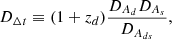 (12)
(12)
with zd representing the lens redshift. Then, DAd, DAs, and DAds refer to the angular diameter distances to the lens, to the source, and between the lens and source, respectively. The time delay, Δtij, is measured from the exhaustive tracking of images fluxes and both the potentials and the source position are determined by a mass model of the system. In this work, we used six lens systems released by the H0LiCOW compilation (Wong et al. 2020): B1608+656, RXJ1131−1231, HE 0435−1223, SDSS 1206+4332, WFI2033−4723 and PG 1115+080, within a source redshift 0.65 < zs < 1.789. We used the likelihood provided by the H0LiCOW collaboration6. According to Wong et al. (2020), the time delay measurements for each lens are uncorrelated. Furthermore, the cited authors computed the Bayes factor between different lenses to confirm the consistency of all measurements.
4. Results and discussion
In this section, we show the results of our statistical analyses assuming the ZKDR and mZKDR distance relations presented in Section 2 and the observational data described in Section 3. For comparison, we also show the results for the standard (FLRW) ΛCDM model. The free parameters in our analysis are the smoothness parameter, α, the mass density parameter, Ωm, the Hubble parameter, H0, the curvature parameter, Ωk (in cases where a curved space is considered) and the absolute magnitude of SNIa Mabs for the analyses that use SNIa data7. We used uniform priors for all parameters, which are shown in Table 2. We sampled our posterior distributions using the EMCEE Python library (Foreman-Mackey et al. 2013)8.
Priors used for each model in the statistical analyses.
Our first general comment, derived from the analysis of all tables and figures is that the PPS dataset is much more constraining than either H0LiCOW or SH0ES+HF. The reason for this lies in the amount of data in the PPS dataset, which contains more data points than SH0ES+HF by one order of magnitude and two orders of magnitude more than H0LiCOW. Consequently, when these datasets are combined in joint analyses, the results are predominantly determined by the PPS contribution. Another point worth highlighting is that our inferred uncertainties are larger than those reported by the H0LiCOW collaboration (Wong et al. 2020). This difference arises primarily from the choice of priors on both Ωm and, in non-flat scenarios, Ωk. However, an inspection of the chains in that analysis reveals that the sampled values pile up against the imposed prior bounds. Since these priors are intended to be non-informative, the prior ranges should be broadened in such cases to ensure a reliable exploration of the parameter space and robust parameter inference.
Within the flat ZKDR framework, our analysis shows that the most constraining dataset for α is PPS, while H0LiCOW provides weaker limits (see Table A.1 and Figures 1 and 2). Besides, the SH0ES+HF dataset fails to impose any meaningful constraints in this framework. Since all results are consistent with α = 1 (ΛCDM model), the most constraining datasets yield higher values for the lower limit of α. Conversely, when examining the flat mZKDR framework, we find that none of the datasets considered here is capable of effectively limiting the value of α. Regarding the matter density parameter, Ωm, our results indicate that within the flat ZKDR framework, PPS imposes particularly stringent constraints on Ωm, while both SH0ES+HF and H0LiCOW provide less restrictive limits. In the mZKDR framework, our analysis shows that constraints derived from the H0LiCOW and SH0ES+HF datasets are comparable to those observed within the ZKDR framework. The PPS dataset, however, provides a more restrictive constraint within the mZKDR framework relative to the other datasets; although we note that this constraint remains notably less stringent than its counterpart obtained within the ZKDR framework. We also note that the mZKDR distance relation indicates slightly higher values for Ωm with respect to ZKDR and ΛCDM. These observed differences between models can be attributed to the parameter degeneracy between α and Ωm in the mZKDR framework (as shown in Eq. 6 and discussed in Sect. 2), a degeneracy that is broken in the ZKDR model (see Eq. 5). Accordingly, the confidence contours in the α − Ωm plane in Figs. 1b and 2b reveal strong correlations for the mZKDR model; whereas for the ZKDR case, only very weak degeneracies appear. Regarding the Hubble constant H0, both SH0ES+HF and PPS datasets provide substantially more stringent constraints than H0LiCOW across all models examined. We also note that when using H0LiCOW data, the estimated H0 values shift to lower values across all models. This effect is more pronounced for ZKDR, which exhibits a tension with the CMB inferred value at the 1.1σ level, less than mZKDR (∼2.1σ) and ΛCDM (2σ)9. However, when PPS data are incorporated, the tension increases to exceed 5σ for all models. On the other hand, only very weak correlations are observed in the H0 − α plane across all datasets, which explains why the modified distance relations considered here cannot solve or alleviate the H0 tension.
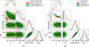 |
Fig. 1. Results of the statistical analyses assuming a flat universe and constant α. The darker and brighter regions correspond to 65% and 95% confidence levels, respectively. The plots in the diagonal show the posterior probability density for each of the free parameters of the scenarios. The left panel shows the results for SH0ES+HF dataset only while the right panel shows the results for PPS. For comparison, the dashed blue curves represent the analyses for the standard (FLRW) ΛCDM model (α = 1). |
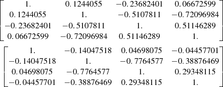
We can then extend our analysis to the non-flat case (see Table A.2 and Fig. 3). We observe that α is only weakly constrained, with similar values obtained across all datasets both in the ZKDR and mZKDR frameworks. Regarding the matter density parameter, Ωm, the constraints for both frameworks remain comparable across all datasets, with those obtained from PPS being the most stringent ones. The difference between these results and those previously described for flat geometries can be attributed to the additional degree of freedom introduced in non-flat models, which consequently generates more parameter degeneracies within the theoretical framework. An interesting feature is that the parameter space inferred for the ZKDR model appears slightly more constrained than that obtained for ΛCDM when using only H0LiCOW data. However, this behaviour might, in fact, be driven by the correlation between α and Ωk10, which is nearly absent in the mZKDR case (see the correlation matrices in Appendix B), as well as by the limited amount of available observational data. With regards to H0, all studied models yield higher values than those obtained for the flat case when using only H0LiCOW data. The difference in the behaviour of the models, can be explained by the addition of an extra parameter (Ωk) which is also correlated with H0 (see Fig. 3a), but this correlation is not apparent when using the different SnIa datasets. In short, we find no evidence that the non-flat ZDKR models could alleviate the Hubble tension since when including PPS the discrepancy with the Planck value remains greater than 5σ across all models. We now turn our attention to the mZKDR1 and mZKDR2 models (see Table 1 for details), which are shown in Table A.3. Following the general trend, α0 (mZKDR1) is more tightly constrained by the PPS dataset, and the same behaviour is observed for β0 (mZKDR2). At the same time, none of the datasets provide meaningful constraints for either α1 or γ. This can be explained since these parameters quantify the time dependence of α, which is more difficult to constrain. However, our results remain consistent with a time-varying α at the 2σ level for both models. With respect to Ωm, the general trend observed in the other models remains, with the PPS dataset providing the most stringent constraints. However, the values of Ωm estimated under the mZDKR1 model are lower than those obtained when assuming the mZKDR2 model. In contrast to the other models studied here, including ΛCDM, when considering the H0LiCOW data, the inferred values of H0 exhibit a smaller shift toward higher values. As a result, the disagreement with the CMB value is at the 2.5σ level for mZKDR1 and 2.6σ for mZKDR2; meanwhile, when all data are employed, they rise above 5σ. In summary, our results do not provide strong evidence that the ZKDR and mZKDR models considered here can alleviate the Hubble tension. Even though Eqs. (5) and (6) do not depend on H0, this parameter enters the calculation of DA as an inverse multiplicative factor. Therefore, some degeneracy in the H0 − α plane is expected, but the statistical analyses performed in this paper show that this degeneracy is small (see Figs. 1, 2 and 3). Finally, we compared the Akaike and Bayesian information criteria (AIC and BIC) to assess which models are favoured by the data. The results presented in Table 3 indicate that there is only weak evidence leaning in favour of ΛCDM against the ZKDR model, whereas the remaining models considered in this work are shown to be strongly disfavoured.
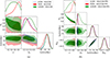 |
Fig. 2. Results of the statistical analyses assuming a flat universe and constant α. The darker and brighter regions correspond to 65% and 95% confidence levels, respectively. The plots in the diagonal show the posterior probability density for each of the free parameters of the scenarios. The left panel shows the results for H0LiCOW data only while the right panel shows the results for both H0LiCOW and PPS data. For comparison, the dashed blue curves represent the analyses for the standard (FLRW) ΛCDM model (α = 1). |
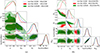 |
Fig. 3. The same as in previous figure for non-flat geometries. |
Estimates of different statistical criteria obtained for each analysed approach.
5. Conclusions
In this study, we examine the impact of small-scale inhomogeneities on the propagation of light from distant sources, with particular emphasis on their implications for the Hubble tension. We employed the Zeldovich-Kantowski-Dyer-Roeder (ZKDR) approximation, along with a modified variant, to model these inhomogeneities. Our analysis encompasses both flat and curved cosmological models, allowing the smoothing parameter within the ZKDR distance relation to vary with redshift. To assess these scenarios, we used current observational data from the Pantheon+ compilation, as well as the SH0ES and H0LiCOW collaborations.
Our main conclusion is that neither the ZKDR approximation, nor its modification can solve or even alleviate the Hubble tension. This result is consistent with findings from previous studies. For instance, Odderskov et al. (2016) investigated the effects of local inhomogeneities in the velocity field on the estimation of H0 at low redshifts by computing the redshift-distance relationships for mock sources in N-body simulations. These results were subsequently compared with those derived from the conventional methodology to estimate H0. Moreover, Miura & Tanaka (2024) explored the inhomogeneities of the universe within the framework of Newtonian cosmology, using the adhesion model for collapsed regions that adhere to the Zeldovich approximation. Through this approach, the authors determine the luminosity distance and redshift of the source by transporting the wave vector along null geodesics, thereby making possible the estimation of H0.
Finally, we underscore that the tension surrounding the H0 measurement remains one of the most pressing unresolved issues in cosmology, with the potential to uncover physics beyond the standard ΛCDM model. Among the various approaches to address this issue, we have explored a possibility that does not rely on introducing new physics, but that is focussed instead on the effects of small-scale inhomogeneities on light propagation. We believe that upcoming and ongoing surveys will provide higher-quality data, especially on time-delay lensing, enabling us to validate or contest the results and conclusions of this work.
Acknowledgments
L.K. and S.L. are supported by grant PIP 11220200100729CO CONICET, grant 20020170100129BA UBACYT and grant SG002 UNLP. J.S.A. is supported by Conselho Nacional de Desenvolvimento Científico e Tecnológico (CNPq) under Grant No. 307683/2022-2 and by Fundação de Amparo à Pesquisa do Estado do Rio de Janeiro (FAPERJ) under Grant No. 299312 (2023).
References
- Abdul Karim, M., Aguilar, J., Ahlen, S., et al. 2025, Phys. Rev. D, 112, 083515 [Google Scholar]
- Aiola, S., Calabrese, E., Maurin, L., et al. 2020, JCAP, 2020, 047 [Google Scholar]
- Alcaniz, J. S., Lima, J. A. S., & Silva, R. 2004, IJMPD, 13, 1309 [Google Scholar]
- Alcaniz, J., Bernal, N., Masiero, A., & Queiroz, F. S. 2021, PLB, 812, 136008 [Erratum: Sci. Rep., 13, 209 (2023)] [Google Scholar]
- Alcaniz, J. S., Neto, J. P., Queiroz, F. S., da Silva, D. R., & Silva, R. 2022, Sci. Rep., 12, 20113 [Google Scholar]
- Balkenhol, L., Dutcher, D., Spurio Mancini, A., et al. 2023, Phys. Rev. D, 108, 023510 [NASA ADS] [CrossRef] [Google Scholar]
- Bolejko, K. 2011, MNRAS, 412, 1937 [Google Scholar]
- Brout, D., Scolnic, D., Popovic, B., et al. 2022, ApJ, 938, 110 [NASA ADS] [CrossRef] [Google Scholar]
- Chen, S.-F., & Zaldarriaga, M. 2025, JCAP, 2025, 014 [Google Scholar]
- Clarkson, C., Ellis, G. F. R., Faltenbacher, A., et al. 2012, MNRAS, 426, 1121 [Google Scholar]
- da Costa, S. S., da Silva, D. R., de Jesus, A. S., Pinto-Neto, N., & Queiroz, F. S. 2024, JCAP, 04, 035 [Google Scholar]
- Dainotti, M. G., Bargiacchi, G., Bogdan, M., Capozziello, S., & Nagataki, S. 2024, JHEAp, 41, 30 [Google Scholar]
- Dashevskii, V. M., & Zel’dovich, Y. B. 1965, Soviet Astron., 8, 854 [Google Scholar]
- DESI Collaboration (Adame, A. G., et al.) 2025, JCAP, 02, 021 [CrossRef] [Google Scholar]
- Di Valentino, E., Mena, O., Pan, S., et al. 2021, Class. Quant. Grav., 38, 153001 [NASA ADS] [CrossRef] [Google Scholar]
- Dinda, B. R., & Maartens, R. 2025, JCAP, 01, 120 [Google Scholar]
- Dinda, B. R., & Maartens, R. 2025, MNRAS, 542, L31 [Google Scholar]
- Efstathiou, G. 2021, MNRAS, 505, 3866 [NASA ADS] [CrossRef] [Google Scholar]
- Efstathiou, G. 2025a, Philos. Trans. A, 383, 20240022 [Google Scholar]
- Efstathiou, G. 2025b, MNRAS, 538, 875 [Google Scholar]
- Foreman-Mackey, D., Hogg, D. W., Lang, D., & Goodman, J. 2013, PASP, 125, 306 [Google Scholar]
- Freedman, W. L. 2021, ApJ, 919, 16 [NASA ADS] [CrossRef] [Google Scholar]
- Freedman, W. L., Madore, B. F., Hoyt, T., et al. 2020, ApJ, 891, 57 [Google Scholar]
- Freedman, W. L., Madore, B. F., Hoyt, T. J., et al. 2025, ApJ, 985, 203 [Erratum: ApJ, 993, 252 (2025)] [Google Scholar]
- Helbig, P. 2020, Open J. Astrophys., 3, 1 [Google Scholar]
- Kalomenopoulos, M., Khochfar, S., Gair, J., & Arai, S. 2021, MNRAS, 503, 3179 [Google Scholar]
- Kantowski, R. 1969, ApJ, 155, 89 [NASA ADS] [CrossRef] [Google Scholar]
- Karwal, T., & Kamionkowski, M. 2016, Phys. Rev. D, 94, 103523 [NASA ADS] [CrossRef] [Google Scholar]
- Khalife, A. R., Zanjani, M. B., Galli, S., et al. 2024, JCAP, 2024, 059 [CrossRef] [Google Scholar]
- Leizerovich, M., Kraiselburd, L., Landau, S., & Scóccola, C. G. 2022, Phys. Rev. D, 105, 103526 [Google Scholar]
- Lewis, A. 2025, JCAP, 2025, 025 [Google Scholar]
- Linder, E. V. 1988, A&A, 206, 190 [NASA ADS] [Google Scholar]
- Lodha, K., Calderon, R., Matthewson, W. L., et al. 2025, Phys. Rev. D, 112, 083511 [Google Scholar]
- Lovick, T., Dhawan, S., & Handley, W. 2025, MNRAS, 536, 234 [Google Scholar]
- Miura, T., & Tanaka, T. 2024, JCAP, 2024, 126 [Google Scholar]
- Negrelli, C., Kraiselburd, L., Landau, S., & Scóccola, C. G. 2020, JCAP, 2020, 015 [Google Scholar]
- Odderskov, I., Koksbang, S., & Hannestad, S. 2016, JCAP, 2016, 001 [Google Scholar]
- Perivolaropoulos, L. 2024, Phys. Rev. D, 110, 123518 [Google Scholar]
- Planck Collaboration VI. 2020, A&A, 641, A6 [NASA ADS] [CrossRef] [EDP Sciences] [Google Scholar]
- Poulin, V., Smith, T. L., Karwal, T., & Kamionkowski, M. 2019, Phys. Rev. Lett., 122, 221301 [Google Scholar]
- Refsdal, S. 1964, MNRAS, 128, 307 [NASA ADS] [CrossRef] [Google Scholar]
- Riess, A. G., Yuan, W., Macri, L. M., et al. 2022, ApJ, 934, L7 [NASA ADS] [CrossRef] [Google Scholar]
- Santos, R. C., & Lima, J. A. S. 2006, ArXiv e-prints [arXiv:astro-ph/0609129] [Google Scholar]
- Schneider, P., Ehlers, J., & Falco, E. E. 1992, Gravitational Lenses (Springer) [Google Scholar]
- Scolnic, D., Brout, D., Carr, A., et al. 2022, ApJ, 938, 113 [NASA ADS] [CrossRef] [Google Scholar]
- Sousa-Neto, A., Bengaly, C., González, J. E., & Alcaniz, J. 2025, A&A submitted, ArXiv e-prints [arXiv:2502.10506] [Google Scholar]
- Suyu, S. H., Marshall, P. J., Auger, M. W., et al. 2010, ApJ, 711, 201 [Google Scholar]
- Tripp, R. 1998, A&A, 331, 815 [NASA ADS] [Google Scholar]
- Wong, K. C., Suyu, S. H., Chen, G. C. F., et al. 2020, MNRAS, 498, 1420 [Google Scholar]
- Zel’dovich, Y. B. 1964, Soviet Astron., 8, 13 [Google Scholar]
Measurements of Baryon Acoustic Oscillations from the DESI collaboration (Abdul Karim et al. 2025), combined with data from the cosmic microwave background and Type Ia supernovae (SNeIa), have challenged the ΛCDM paradigm indicating a potential evolution in the dark energy equation of state. These results are currently the subject of debate (Efstathiou 2025b), with both parametric and non-parametric analyses yielding divergent conclusions (DESI Collaboration 2025; Dinda & Maartens 2025; Sousa-Neto et al. 2025; Lodha et al. 2025).
Most studies refer to the distance relation incorporating these concepts as the Dyer-Roeder approximation. Here, we follow Alcaniz et al. (2004) and refer to it (see Eq. (5)) as the Zeldovich-Kantowski-Dyer-Roeder (ZKDR) distance relation to recognise the contributions of the original authors on this topic.
Each dataset contains the B band magnitude from SNIa and its corresponding redshift together with the corresponding distance modules from Cepheid data.
The entire compilation consist of 1701 data points. However, for the purpose of testing cosmological models only the points at redshift z > 0.01 are considered.
Recent studies Dainotti et al. (2024), Lovick et al. (2025), have explored alternative likelihoods for the Pantheon+ dataset, including a Student’s t-distribution. However, the preferred values of the degrees of freedom are sufficiently large that the distribution is nearly Gaussian, yielding only minor effects on cosmological parameter estimates and the Hubble tension. We repeated our analysis using this alternative likelihood and found slightly tighter constraints only for the ΛCDM model (for the ZKDR and mZKDR models, the Gaussian distribution is more constraining), while our main conclusions remained unchanged. Therefore, for consistency with the standard methodology adopted in most SNIa cosmological studies, we present our results assuming a Gaussian likelihood.
In cases where a varying α(z) is assumed in the mZKDR equation, the free parameters of the analysis are detailed in Table 1.
The sampling algorithm is Affine Invariant Markov chain Monte Carlo Ensemble Sampler while the convergence criterion is based on the autocorrelation time. For post-processing of the chains and the confidence contours, we used the GetDist library (Lewis 2025).
Here Nσ is calculated using the ‘rule of Thumb’ which quantifies the disagreement between two inferred parameters μA/B with variance σA/B in terms of 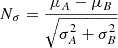 .
.
This fact may partially break the geometric degeneracies among Ωm, Ωk and H0, leading to a more localised likelihood and consequently narrower marginalised constraints on these parameters.
Appendix A: Result tables
The subsequent tables present the results obtained from the different statistical analyzes performed in this study.
Results from our statistical analysis for the ZKDR and mZKDR approximations and (FLRW) ΛCDM with Ωk = 0 and α constant.
The same as in the previous table for non-flat geometries and assuming α constant.
The same as in the previous table for flat geometries and assuming α as function of z.
Appendix B: Correlation matrices
The following matrices present the parameter correlations for the non-flat ZKDR and non-flat mZKDR models, using exclusively H0LiCOW data. The parameters are ordered as α, Ωm, Ωk, and H0. In the case of the non-flat ZKDR model (upper one), a mild correlation between α and Ωk is observed, whereas this correlation is negligible in the mZKDR model.
All Tables
Estimates of different statistical criteria obtained for each analysed approach.
Results from our statistical analysis for the ZKDR and mZKDR approximations and (FLRW) ΛCDM with Ωk = 0 and α constant.
The same as in the previous table for non-flat geometries and assuming α constant.
The same as in the previous table for flat geometries and assuming α as function of z.
All Figures
|
Fig. 1. Results of the statistical analyses assuming a flat universe and constant α. The darker and brighter regions correspond to 65% and 95% confidence levels, respectively. The plots in the diagonal show the posterior probability density for each of the free parameters of the scenarios. The left panel shows the results for SH0ES+HF dataset only while the right panel shows the results for PPS. For comparison, the dashed blue curves represent the analyses for the standard (FLRW) ΛCDM model (α = 1). |
| In the text | |
|
Fig. 2. Results of the statistical analyses assuming a flat universe and constant α. The darker and brighter regions correspond to 65% and 95% confidence levels, respectively. The plots in the diagonal show the posterior probability density for each of the free parameters of the scenarios. The left panel shows the results for H0LiCOW data only while the right panel shows the results for both H0LiCOW and PPS data. For comparison, the dashed blue curves represent the analyses for the standard (FLRW) ΛCDM model (α = 1). |
| In the text | |
|
Fig. 3. The same as in previous figure for non-flat geometries. |
| In the text | |
Current usage metrics show cumulative count of Article Views (full-text article views including HTML views, PDF and ePub downloads, according to the available data) and Abstracts Views on Vision4Press platform.
Data correspond to usage on the plateform after 2015. The current usage metrics is available 48-96 hours after online publication and is updated daily on week days.
Initial download of the metrics may take a while.