


| Issue |
A&A
Volume 711, July 2026
|
|
|---|---|---|
| Article Number | A181 | |
| Number of page(s) | 17 | |
| Section | Stellar structure and evolution | |
| DOI | https://doi.org/10.1051/0004-6361/202659217 | |
| Published online | 14 July 2026 | |
Halo stars harbour few wide ultracool companions
1
Instituto de Astrofísica de Canarias (IAC), Calle Vía Láctea s/n, 38200, La Laguna, Tenerife, Spain
2
Departamento de Astrofísica, Universidad de La Laguna (ULL), Avenida Astrofísico Francisco Sánchez s/n, 38206, La Laguna, Tenerife, Spain
3
Department of Physics and Astronomy, The University of Western Ontario, 1151 Richmond St, London, ON, N6A 3K7, Canada
4
Institute for Earth and Space Exploration, The University of Western Ontario, 1151 Richmond St, London, ON, N6A 3K7, Canada
★ Corresponding author: This email address is being protected from spambots. You need JavaScript enabled to view it.
Received:
30
January
2026
Accepted:
28
May
2026
Abstract
Aims. Our goal is to provide a wide ultracool companion frequency for metal-poor halo stars for the first time.
Methods. We selected nearby halo stars with spectroscopically determined high proper motions and metallicities. We collected first-epoch deep J-band imaging around these stars. We visually compared these images with optical images from public surveys, and the stars with nearby faint sources beyond the optical survey limit were followed up by deep J-band imaging with baselines of two to four years. We searched for comoving sources between the two epochs.
Results. Our observation reached an average depth of Jlim = 22.8 and 23.0 mag (Vega) in the first and the second epoch, respectively, enabling us to detect esds earlier than type esdT0 at a distance up to 250 pc. With this depth, we found no bona fide wide ultracool comoving companions to a nearby metal-poor halo star within a typical projected separation range of a few hundred to a few thousand au from the star. We place an upper limit of the frequency of wide ultracool companions to metal-poor halo stars of 4.0% at a confidence level of 90%. With four stellar comoving companions found and confirmed by Gaia, we derived a wide stellar companion frequency of 6.1+7.2−4.0% at a confidence level of 90%.
Conclusions. We conclude that wide ultracool companions are rare around metal-poor halo stars, with a frequency marginally lower than that of wide stellar companions. We claim that no metallicity dependence is found for the wide ultracool companion frequency around stars so far. Formation and retention processes in binary systems are likely to operate less efficiently for ultracool secondaries.
Key words: proper motions / binaries: general / stars: late-type / stars: low-mass / stars: Population II / subdwarfs
© The Authors 2026
 Open Access article, published by EDP Sciences, under the terms of the Creative Commons Attribution License (https://creativecommons.org/licenses/by/4.0), which permits unrestricted use, distribution, and reproduction in any medium, provided the original work is properly cited.
This article is published in open access under the Subscribe to Open model. This email address is being protected from spambots. You need JavaScript enabled to view it. to support open access publication.
1. Introduction
Ultracool dwarfs (UCDs) are objects with spectral types later than M7.0 V and effective temperatures Teff ≲ 2700 K (Kirkpatrick et al. 1997; Kirkpatrick 2005). Owing to their inefficient or absent sustained hydrogen fusion, halo UCDs serve as valuable fossil tracers of the early Milky Way. Consisting of pristine materials, halo UCDs are metal poor, and they therefore serve as natural laboratories for testing low-metallicity cold atmosphere models. Based on their spectral features, they are classified into three metallicity subclasses: normal subdwarf (sd), extreme subdwarf (esd), and ultra subdwarf (usd; Lépine et al. 2007; Zhang et al. 2017b; Burgasser et al. 2025b). Late-type M subdwarfs were first detected in the first generation of digitized surveys almost three decades ago (Gizis et al. 1997; Scholz et al. 2004; Lodieu et al. 2005), followed shortly thereafter by the discoveries of L subdwarfs (Burgasser et al. 2003; Lépine et al. 2003).
The well-constrained properties of the stellar primary and the wide separation that enables the secondary to be resolved mean that halo ultracool subdwarfs as wide companions to stars or evolved stars are considered valuable benchmarks. Several such systems have been identified in recent years; for example, HD 114762B as a late-M subdwarf wide companion to the F subdwarf HD 114762A (Bowler et al. 2009), Wolf 1130C as a late-T subdwarf wide companion to the M subdwarf-white dwarf binary system Wolf 1130AB (Mace et al. 2013, 2018; Burgasser et al. 2025a), GJ 660.1B as a late-M subdwarf wide companion to the early-M subdwarf GJ 660.1A (Aganze et al. 2016), Gaia J045245.87−360843.8 as the early-L subdwarf wide companion to the early-M subdwarf Gaia J045238.82−361001.3 (Zhang 2019), and VVV J125641.09−620203.8 as the early-L subdwarf wide companion to the white dwarf VVV J125644.42−620208.1 with a progenitor mass of 1.9 ± 0.4 M⊙ (Zhang et al. 2019b, 2024b).
Although a small number of halo wide ultracool companions to stars have been confirmed, the frequency of wide ultracool companions in the halo stellar population remains poorly constrained, and it is unclear how metallicity affects the formation of these systems. Halo stars account for a small portion of the whole stellar population, and it is therefore necessary to cover a large volume for a statistically significant sample. However, the intrinsic faintness of UCDs, especially that of ultracool subdwarfs, prevents us from detecting them at large distances. In comparison, several studies have investigated wide stellar companions to metal-poor stars and found frequencies ranging from a few percent to ∼10–20% (Zapatero Osorio & Martín 2004; Jao et al. 2009; Zhang et al. 2013; Ziegler et al. 2015; Hwang et al. 2021; Lodieu et al. 2025). Others reported the frequency of wide ultracool companions of solar-metallicty stars and young stars to be a few percent (Metchev & Hillenbrand 2009; Chinchilla et al. 2019; dal Ponte et al. 2020).
To fill this gap and provide valuable constraints on the formation and evolution of such systems, we carried out a dedicated survey to identify comoving wide ultracool companions to metal-poor stellar primaries. It involved two-epoch deep imaging of a large sample of selected metal-poor halo stars. We obtained the images in the near-infrared (NIR) wavelengths where UCDs are relatively bright.
This work is structured as follows: Section 2 describes the sample selection, observation details, and data reduction. The main results are presented in Sect. 3. In Sect. 4 we compare our results with those from the literature and discuss their implications. Section 5 summarises the work.
2. Observations
2.1. Sample selection
We selected 66 bright halo stars observable from the Canary Islands, with spectroscopically determined metallicity [Fe/H] < − 1.5 dex, from the 1447 stars in the catalogue of Carney et al. (1994). This catalogue was based on historical proper-motion surveys, implying that the selected stars exhibit sufficiently large proper motions to be detectable with earlier observational techniques. As a result, the sample consists of nearby relatively bright and highly reliable halo members. In addition, the use of high-resolution spectroscopy provides robust metallicity measurements.
To ensure that potential ultracool companions would be detectable, all objects of the sample are within 250 pc, and seven objects are within 100 pc. These stars have effective temperatures from 4600 to 6300 K. The total proper motions of these targets range from 193 to 2204 mas yr−1, allowing us to measure motions from the ground over the few-year baseline between the first and second epoch. The information about these 66 targets is listed in Table A.1.
2.2. First-epoch observation
For the first epoch, the observations were conducted under service programmes GTC53-20B and GTC65-21A (PI: N. Lodieu) during 2020 and 2021. Three targets with two records in the first-epoch modified Julian date (MJD) in Table A.1 were observed twice in this epoch. We kept the images with a higher quality from the two epochs.
We used the Espectrógrafo Multiobjeto Infrarrojo (EMIR; Garzón et al. 2022) on the 10.4 m Gran Telescopio Canarias (GTC) located at the Spanish island of La Palma. EMIR is a common-user wide-field near-infrared camera installed on one of the GTC’s Nasmyth foci. EMIR was equipped with a Teledyne HAWAII-2 HgCdTe near-infrared optimised chip of a size of 2048 × 2048 pixels. The field of view (FoV) of EMIR is  and the pixel scale is
  pix−1. The smallest total proper motion of the 66 targets corresponds to a minimum displacement of 3 pixels on the EMIR detector over approximately a three-year baseline between the first and second epoch. This motion is sufficiently large to be detected and measured with high significance and good precision (> 10σ), as the centroid position error of the point spread function (PSF) for the faintest source at S/N = 3 can be determined to about a quarter pixel with EMIR.
We used the J-band filter because the J band is less affected by strong collision-induced absorption in the low-metallicity ultracool atmosphere and the sky-background emission is lower than in the H and K bands. We deployed a standard seven-point dithering pattern with an offset of 25″, and the on-source exposure time for each object was 60 s × 7 dithering × 3 cycles = 1260 s. Even though all the primaries are extremely bright for a 10 m class telescope and would be saturated, the single-exposure time was kept to 60 s to make compromises with a reasonable amount of overheads. The actual seeing conditions ranged from  to
to  . There were no constraints on the Moon phase, but the Moon was required to be at least 30° away from the target.
Two targets, G 103−50 and G 27−8B, were not observed with the configuration. They are denoted with an asterisk in the first-epoch MJD t1 column in Table A.1. The first had a very short exposure of 5 × 5 s = 25 s and the second had no dithering, and the background could therefore not be subtracted well enough. The images were not deep, but we still reduced them to extract as much information as possible.
2.3. Data reduction
The 2D EMIR frames were preliminarily reduced by the EMIR default pipeline PyEmir1. The pipeline performed bad-pixel masking, flat-fielding, sky subtraction using the dithering pattern, and stacking.
To avoid effects from distorted stars on the astrometry in the central region of interest, astrometric calibration was applied after the edge of the frames was cut. We then used the Astrometry.net script (Lang et al. 2010) to solve the astrometry for the final stacked and cropped images.
2.4. Target selection for the second-epoch observation
We visually examined the images to determine whether any faint sources were close by. We created cutouts with sizes of 90″ × 90″ centred at the stars. This cutout size was chosen to exclude sources at the edge that were substantially affected by instrumental aberrations and distortions. The projected physical sizes of the cutout were set to 90 d au × 90 d au, where d is the distance of the star in parsecs. Thus, the maximum projected separation explored for each target ranged from a few hundred to a few thousand au.
We compared these first-epoch images with the Panoramic Survey Telescope and Rapid Response System (Pan-STARRS; Chambers et al. 2016) coloured images with their red, green, and blue (RGB) channels corresponding to the y, z, and i bands, respectively. We used these three reddest bands of Pan-STARRS to maximise the sensitivity of the ultracool objects. The sources with a Pan-STARRS detection would have been recognised moved significantly if they are comoving companions, thanks to the large baseline (6−11 years) between the Pan-STARRS’s epoch and our first epoch.
We recovered four stellar companions in the Washington Double Star Catalog: G 79−56 with its companion LSPM J0341+0923W, discovered by Skiff B.A.; BD+00°2058A with BD+00°2058B, discovered by Herschel J.F.W.; G 214−1 with G 214−1B, discovered by Zapatero Osorio & Martín (2004); and G 27−8 with G 27−8B discovered by Luyten (1979). Their common proper motions were confirmed by Gaia (Gaia Collaboration 2020). We found no other faint sources with red Pan-STARRS counterparts that shared the proper motion with the primary. For the second-epoch observation, we therefore selected 28 targets whose deep images exhibited close-by faint sources that were not detected by Pan-STARRS, which might be an ultracool comoving companion to the star.
2.5. Second-epoch observations
For the second epoch in 2024, we observed 21 out of these 28 targets with one repetition (G 241−41) with GTC/EMIR+, which is the upgraded GTC/EMIR with a new HAWAII-2RG detector with the same size, pixel scale, and orientation, under programme GTC45-24A (PI: N. Lodieu). Two of these targets (BD+42°2667 and G 241−4) were observed during the commissioning of GTC/EMIR+ earlier on 30 August 2023. The observational setup and data reduction procedures were kept consistent with those of the first epoch, but the stacking offsets in the second epoch were determined automatically by the pipeline and not manually using the imexam task. The actual seeing conditions ranged from  to
to  .
.
2.6. Comovement detection
Figure B.1 presents the deep GTC/EMIR J-band images covering FoVs of 90″ × 90″ for all the 21 targets in both epochs. The images are displayed in a logarithmic scale to enhance the visibility of faint features, along with the corresponding difference images. The difference frames are significantly affected by background contamination caused by diffused light from the bright central star, making them suboptimal for identifying faint comoving sources. To overcome this, we also visually inspected the two-epoch images by blinking them in different scales (linear, logarithmic, and asinh) using SAOImage DS9.
3. Results
We recovered four comoving stellar companions (indicated in Table A.1). Only one comoving ultracool candidate was identified, whose primary is BD+02°3375. This system was selected for further investigation.
3.1. BD+02°3375
We identified an extremely faint source at coordinates 17h39m45 87 +2°25′08
 26 (epoch MJD 60450.09), located north-east of BD+02°3375, which appears to share the proper motion of the star (top panel of Fig. 1). Instead of performing independent astrometric solutions for both epochs, which would introduce astrometric uncertainties twice, we adopted a relative astrometry approach at the pixel level using a single reference frame from one epoch. This method minimises the impact of instrumental aberrations and distortions, particularly because the instrument configurations were nearly identical for both epochs.
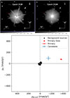 |
Fig. 1. Top: Two epochs of GTC/EMIR J-band images of BD+02°3375 in logarithm count scale. The positions of the comoving companion candidate are pointed out by red arrows. The motion is not visible in the difference image of Fig. B.1. Bottom: Proper motion diagram of the sources. The proper motion of the primary (red cross) agrees well with Gaia (red star) within the uncertainties. The background sources extracted by daofind and by hand have almost zero proper motion (black dots). The candidate (blue cross) has a significant proper motion compared to the background sources, but is not comoving with the primary. |
We used the Image Reduction and Analysis Facility (IRAF; Tody 1986) task daofind to extract bright field stars and then used the task xyxymatch to create a list of matched coordinates (the number of matched stars normally is a few hundred). We manually measured the faint-source position using imexam and imcentroid. We rotated the image using rotate with the primary star as the rotation centre, and we subtracted the rotated image from the original frame to test whether this approach might help us to leverage the effects of stray light and diffraction spikes around the primary. Then, we fitted the shift, rotation, linear magnification, and aberrations of the centre part of both images using the task geomap. At the end, the task geoxytran transformed all the coordinates of one epoch into the reference frame of the other epoch using the parameter derived by geomap.
Although it has a motion with respect to the background at a significance of 5σ and is in a similar direction of BD+02°3375, the proper motion (μα cos δ = −146 ± 37 mas yr−1, μδ = +95 ± 36 mas yr−1) is different from that of the star (μα cos δ = −377 ± 10 mas yr−1, μδ = +71 ± 8 mas yr−1; from EMIR astrometry) at a significance level of 6σ (bottom panel of Fig. 1). The criteria used by Montes et al. (2018) to distinguish physical (bound) from optical (unbound) systems are a ratio of the proper motion value difference to the primary proper motion μ ratio < 0.15, and a proper motion position angle difference ΔPA < 15°. Our candidate pair has μ ratio = 0.60 and ΔPA = 22.4°. We hence discarded the comoving scenario.
3.2. Completeness
3.2.1. Depth
We performed aperture photometry using Photutils (Bradley et al. 2024) to determine the depth of the GTC/EMIR images. We measured the average full width at half maximum (FWHM) of each image by fitting a 2D Gaussian profile for each source extracted by DAOStarFinder, which is based on the algorithm by Stetson (1987). We used apertures with radii of 1.2 times of the FWHM of each image and sky annuli with inner radii of 4″ and outer radii of 6″. As photometric references, we selected all 2MASS sources with J-band magnitudes fainter than 14.0 mag and located within 70″ of the image centres.
For images containing at least four such reference stars, we determined the 3σ limiting J-band magnitude by estimating the background fluctuation within a sky aperture of the same size. In the first epoch, our GTC/EMIR images reach a 3σJ-band limiting magnitude of 22.8 mag on average. For the second epoch, it is about 23.0 mag, likely due to both the detector upgrade and improved average seeing conditions.
To estimate the latest spectral type of metal-poor UCDs detectable at the GTC/EMIR limiting magnitude of the first epoch Jlim = 22.8 mag, we shifted known esds with trigonometric parallaxes and similar metallicities to distances at which their apparent magnitudes matched Jlim (Fig. 2). The sample includes the benchmark extreme metal-poor T dwarf WISEA J181006.18−101000.5 (WISE1810−10), another benchmark late-type sdT or esdT Wolf 1130C, the mid-type esdT CWISE J221706.28−145437.6 (WISE2217−14), and two late-type esdLs 2MASS J05325346+8246465 (2M J0532+82) and 2MASS J06164006−6407194 (2M J0616−64).
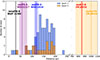 |
Fig. 2. Target distance histogram compared with maximum detectable distances (solid coloured lines) for different spectral types of extreme subdwarfs with low metallicities at the first-epoch GTC/EMIR J-band depth of 22.8 mag. The coloured shades indicate the uncertainty of the maximum detectable distances, which mainly result from the uncertainties of the parallax measurements. |
The benchmark WISE1810−10 is the closest esdT ( pc; Lodieu et al. 2022), and it has the most precise metallicity measured among its kind ([Fe/H] = −1.7 ± 0.2 dex; Zhang et al. 2025b). Given the WISE1810−10 J-band magnitude of 17.3 mag and a spectral type determined from esdT0 (Schneider et al. 2020) to esdT3 (Burgasser et al. 2025b), we could have detected esdT3 objects similar to WISE1810−10 at a maximum distance of
  pc with the aforementioned mean depth, following the inverse-square law. The same calculation was made for the rest; the photometric uncertainty and the parallax uncertainty were all taken into account. Wolf 1130C has metallicity and trigonometric parallax from its primary (an sdM or esdM) and has been classified from sdT8 (Mace et al. 2013) to (e)sdT6 (Burgasser et al. 2025b). WISE2217−14 has a trigonometric parallax of 48 ± 13 mas and signs of extremely low metallicity (Zhang et al. 2025b,a). It has a spectral type of esdT5.5 (Meisner et al. 2023). 2M J0532+82 was classified from esdL7 (Zhang et al. 2013) to esdL8 (Burgasser et al. 2025b) and has a precise distance of 24.56
 pc from Gaia. 2M J0616−64 has a large uncertainty on the spectral type classification from esdL6 (Kirkpatrick et al. 2010; Zhang et al. 2017b) to esdT0 (Burgasser et al. 2025b) and also has an uncertain distance of 50
 pc (Faherty et al. 2012).
Figure 2 shows that our observations are sensitive to all potential esd companions with spectral types earlier than esdT0 within 250 pc. For early-type esdTs, the detection completeness is estimated at approximately one-third of the whole sample. The sensitivity is insufficient to assess the presence of late-type esdTs or esdYs across the majority of the sample.
3.2.2. Spatial coverage
All of the target stars are too bright to not saturate even in the 60 s GTC/EMIR individual exposures. The stellar flux increases exponentially when the magnitude decreases, and the wing of the PSF approximately follows a 2D exponential profile. The saturation radius of the star is therefore expected to decrease roughly as the square root of the magnitude. By checking the image, we found that regions with an analog-to-digital unit (ADU) count ≳30 000 lose linearity. We empirically fitted the saturation radius in arcseconds with the J-band magnitude of the star  . This relation implies that stars fainter than 13.0 mag in the J band will not saturate in these exposures, which is consistent with the photometric analysis.
In practice, the PSFs are more complex and are affected by multiple factors, including atmospheric seeing and optical diffraction. To remain conservative in our analysis, we defined the innermost detectable separation for ultracool comoving companions as 2Rsat. When Rsat was smaller than the worst seeing allowed in the observation, that is,  , we instead fixed the innermost separation to
  . At the distance to each star, this angular threshold translates into a physical projected separation in au. Combined with the outer boundary set by the cutout size, these limits define the range of separations that we probed for each target (Fig. 3). Except for some very close-by and bright sources, the physical projected separation ranged from ∼500 up to ∼8000 au from the central stars.
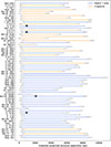 |
Fig. 3. Explored projected physical separation ranges (au) for comoving companions of each target, with objects ordered by increasing right ascension from bottom to top. Objects with two epochs of GTC/EMIR observations are shown in orange, and the rest are plotted in blue. The black stars show the four identified known stellar companions. |
3.3. Frequency of wide stellar companions
Four of our 66 stars have Gaia-confirmed comoving stellar companions, including G 27-8B, which had failed to have deep image in the first epoch. Although Gaia has a good completeness of M7 dwarfs at a distance of 100 pc (Gaia Collaboration 2021), we calculated the Gaia limit for metal-poor subdwarfs. According to the absolute G magnitude of esdMs with a metallicity [Fe/H] < −1.0 dex derived from Table 4 of Zhang et al. (2021), together with the Gaia limit of G = 20.7 mag (Gaia Collaboration 2016), we inferred that Gaia can detect an early-type esdM at a distance of 100–200 pc.
Mid- to late-type esdMs at distances of ∼200 pc, which are below the Gaia detection limit, can be readily detected by Pan-STARRS (Zhang et al. 2013). Nevertheless, none were found during the visual comparison between Pan-STARRS and our first-epoch observations.
If it were complete until late-type esdM companions, the wide stellar companion frequency of the halo stars would be pstar = k/n = 4/66 = 6.1%. Assuming a binomial distribution to calculate the two-sided 90% confidence interval (statistical significance α = 0.1) of pstar, we have
 (1)
(1)
which yields  .
.
3.4. Upper limit of wide ultracool companion frequency
No faint UCD companions were confirmed to be comoving, and we therefore derived an upper limit on the true wide ultracool companion frequency p at a confidence level of 90%, assuming the same binomial distribution as for calculating the stellar companion frequency. Since two targets did not reach a depth for probing the UCDs in the first epoch and seven targets might still harbour faint companions but were not observed in the second epoch, there were n = 66 − 2 − 7 = 57 independent trials. We have
 (2)
(2)
yielding a true frequency with an upper limit of pUCD ≤ 4.0%. This frequency limit only applies to the complete sample with spectral types earlier than esdT0.
4. Discussion
We compared our results with literature samples spanning a range of physical properties in order to explore potential dependences of the wide ultracool companion frequency. A summary of this discussion is provided in Table 1.
Companion frequencies from this work and the literature.
4.1. Metallicity and age dependence
Our pUCD agrees with the 2σ limit frequency of wide (28–1590 au) brown dwarf (BD) companions to young solar-type stars of  (Metchev & Hillenbrand 2009). Similarly, in Upper Scorpius, Chinchilla et al. (2019) found a comparable ∼3% frequency of wide (400–9000 au) companions with candidate spectral types M to L around young stars. Our result is also consistent with the wide (1000–24 000 au) star-UCD candidate binary fraction of 2–4% (dal Ponte et al. 2020).
These consistencies do not reveal the effect of metallicity or age on the formation of binaries that consist of a solar-type star and an ultracool companion. Their pronounced paucity remains universal at different metallicities and ages.
4.2. Dependence on the mass of the primary
Our pUCD agrees with the wide-companion frequency to metal-poor late-M and L subdwarfs reported by González-Payo et al. (2021), who measured a multiplicity rate of  for sdMs and
  for esdMs, and who set an upper limit of 5.3% for usdMs, although over projected separations of ∼1000−140 000 au. Since their sample only included one companion to an esdM (which is an esdL) and no companion to usdMs, the multiplicity rates for esdMs and usdMs effectively represent their ultracool companion frequencies or limits. As a result, there is no evidence that the low ultracool companion frequency in the metal-poor regime is dependent on the primary mass.
Regardless of the metallicity, Winters et al. (2019) revealed that for nearby M dwarfs within 25 pc, the wide BD companion frequency is 1.3 ± 0.3% with a separation between 2 and 300 arcsec, which is equivalent to from a few au to a maximum of 7500 au. The consistency of this value and our result supports the conclusion that there is currently no clear evidence that low metallicity affects the wide ultracool companion frequency, even across different primary stellar types from FGK stars to M dwarfs.
4.3. Dependence on the separation of the primary and secondary
Although no frequency of close ultracool companions to metal-poor stars was reported so far, we can infer it from other studies. Marcy & Butler (2000) and Grether & Lineweaver (2006) found that < 1% of solar-type stars harbour BDs in close orbits; this is the so-called the BD desert. Sahlmann et al. (2011) set the upper limit of the frequency of close (< 10 au) BD companions around solar-metallicity solar-type stars to 0.6%.
According to Moe et al. (2019), the close binary rate of solar-type stars has strong anti-correlation with the metallicity of the primary: it increases from 24 ± 6% at field metallicity to 53 ± 12% at a metallicity of −3 dex by a factor of two. Close companions mostly form via disk fragmentation, and this instability is more likely to occur under conditions of lower metallicity because the infall rates from hotter cores are higher and the temperatures of the optically thick disks are lower. Even with the bold assumption that the close BD companion frequency follows this trend with metallicity, the frequency of close BD companions to metal-poor stars will not exceed a few percent, which still agrees with our result of the wide ultracool frequency.
Giant planets serve as analogues to UCDs, although they may form in a different manner than more massive UCDs near a metal-poor star. Mortier et al. (2012) claimed that giant planets are rare (≤2.36%) around metal-poor stars with a metallicity of [Fe/H] < −0.7 dex, which is comparable to our inferred low frequency for close BD companions to metal-poor stars. However, if the fact that close BD companions appear to be rarer than giant planets (Grether & Lineweaver 2006) still holds for metal-poor stars, we would expect an even lower frequency for the close ultracool companion frequency. These comparisons suggest that separation probably does not strongly affect the ultracool companion frequency around metal-poor stars overall.
4.4. Stellar companion frequency
Although previous studies reported varying results on stellar companion frequencies for metal-poor stars, our pstar is consistent with them within the uncertainties and considering incompleteness effects. Using infrared speckle interferometry on the same sample of Carney et al. (1994), together with that of Norris (1986), Zinnecker et al. (2004) derived a binary frequency of 6−20% for halo stars with metallicities [Fe/H] < −1.6 dex and separations larger than 10 au. The 6% estimate corresponds to a K-band flux-ratio detection threshold of 0.1, while the 20% estimate assumes a threshold of 0.01. To enable a direct comparison with our result, we excluded companions within 300 au of their background-corrected sample at the 0.01 K-band flux ratio threshold, yielding a frequency of ∼9% for binaries wider than 300 au. This is an approximation because triple systems are included. Our result is consistent with this value. Lodieu et al. (2025) reported an upper limit of 3% for stellar companions to mid-F- to early-K primaries with a metallicity of [Fe/H] < −1.5 dex and projected separations between 8 and 10 000 au. Although this value is relatively low and might be strongly affected by incompleteness, the lower bound of our result is consistent with this limit. Hwang et al. (2021) reported a relatively low wide (1000 to 10 000 au) binary fraction for metal-poor FG stars with metallicity ∼ − 1.5 dex of ∼1% using LAMOST data, which is likewise consistent with our findings considering the uncovered gap between 100 to 1000 au. Our result further agrees with the 4.5% frequency reported by Lodieu et al. (2025) after correcting for the primary metallicities, based on the overall wide-binary fraction of 13−15% for stars with metallicities between −3.5 and 0.0 dex and projected separations between 32 and 57 000 au from Zapatero Osorio & Martín (2004). Our result also agrees with the lower bound of the wide (> 100 au) binary frequency of 2.41% for KM red subdwarfs in different metallicity subclasses reported by Zhang et al. (2013). Jao et al. (2009) provided a high multiplicity rate of metal-poor KM-type cool subdwarfs of 26 ± 6% using speckle interferometry. Of the 26%, 12% are binaries at separations smaller than 100 au, and the remaining 14% are wide binaries with separations larger than 100 au. Ziegler et al. (2015) probed wide companions to metal-poor FGKM-type subdwarfs using high-resolution adaptive optics imaging and included previously recorded wide companions. They found a multiplicity rate of 12.5 ± 1.9%, and these systems have projected separations ranging from 105 ± 12 to 79 156 ± 9046 au. At its upper bound, our wide companion frequency is consistent with both studies. Two factors may account for this agreement. First, similar to Zinnecker et al. (2004), these high-resolution studies effectively covered the separation range from 100 to a few hundred au that were not probed by our seeing-limited observations. Second, they targeted lower-mass primaries that were not studied by this work.
Following the review of wide stellar companion frequencies reported in the literature, we only adopted our own measurement pstar for metal-poor halo stars. Based on this reference, the wide ultracool companion frequency pUCD is marginally lower than that of wide stellar companions pstar.
4.5. Primary mass and separation
As discussed above, the primary-secondary separation may have little effect on the ultracool companion frequency for metal-poor FGK stars. In the metal-poor M subdwarf regime, the wide companion frequency of  (González-Payo et al. 2021) is comparable with the frequency of intermediate-separated (a few to some tens of au) companions to M subdwarfs of ∼3% measured by Riaz et al. (2008) and Lodieu et al. (2009) using the Hubble Space Telescope and lucky imaging, respectively.
In addition, although lacking metallicity constraints, but with tighter limits on secondary masses, Gaia Collaboration (2023) proposed ∼0.3% for the frequency of close BDs to M dwarfs with periods shorter than about 1000 days, that is, with semi-major axes shorter than 1 to 2 au. Several studies also agreed in their low frequencies of BD companions to M dwarfs of 2.3% to 2.8% at intermediate separations of a few to some tens of au (Dieterich et al. 2012; Bowler et al. 2015; Susemiehl & Meyer 2022). Taken together, these results suggest that separation might affect the ultracool companion frequency around metal-poor stars little for all spectral types, and for M dwarfs across a range of metallicities.
4.6. Rarity of wide ultracool companions
We found that wide ultracool companions are rare around stars. This rarity appears to be consistent for all primary spectral types, metallicities, and companion separations. The formation of wide ultracool companions might be naturally suppressed in core fragmentation, as the efficiency of fragmentation decreases towards the low-mass end (Chabrier 2003; Bate 2012), and extreme mass-ratio (q < 0.1) systems represent only a small fraction of the outcomes of the formation process (Bate 2012).
In particular, even if metal-poor environment favours the formation of wide ultracool companions, they have gone through a long cooling process of ∼10 Gyr. The degeneracy of BDs and very low-mass stars in the spectral type range of late-M to L naturally breaks: the majority of substellar objects have been cooled to very late spectral types (Zhang et al. 2019a), which are beyond the detection limit of this research, leaving a spectral type gap from early-L to early-T that is barely filled by transitional BDs. These transitional BDs occupy a very narrow mass range and thus account for a small portion of the population (Zhang et al. 2017a, 2018, 2019a).
In addition, halo wide binaries may not be stable enough to survive the interstellar interactions through their lifetime. For binaries with total masses of 1 M⊙ and semi-major axes of 1000 and 10 000 au, the simulation yields probabilities of ∼90% and ∼20% that they survive for 10 Gyr, respectively (Weinberg et al. 1987). Our star-UCD systems might be more easily disrupted at lower total binding energies because of the high-mass ratio at a certain total mass.
5. Conclusion
We did not identify any bona fide ultracool comoving companion to all 57 halo stars. We concluded that the wide ultracool companion frequency pUCD with companion spectral types earlier than esdT0 around halo metal-poor stars within a separation range of typically a few hundred au up to a few thousand au, is lower than 4.0% at a confidence level of 90%.
This frequency is marginally lower than the wide stellar companion frequency around halo metal-poor stars, for which we found  using the total 66 samples. Given the current uncertainties, we found no statistically significant evidence of any dependence of the wide ultracool companion frequency on metallicity, separation, and primary mass. Ultracool companions appear to be rare throughout the physical parameter space we explored.
We speculated that for the halo population, most brown dwarfs might have cooled to very late spectral types and thus fall below our detection limits of ∼esdT0. The resulting low upper limit of pUCD might therefore only reflect the small fraction of transitional brown dwarfs, which occupy a narrow mass range. More generally, ultracool companions might be intrinsically disfavoured in formation, and wide binary systems in the halo might have a reduced survival probability over their long lifetimes.
Although seven of our targets with potential faint companions currently lack a second epoch, the very low upper limit on the frequency of wide ultracool companions to halo stars implies that a survey-driven strategy is more effective than continued deep NIR imaging of individual targets, even with a 10 m class telescope. In this context, the combination of ongoing and forthcoming deep NIR surveys such as Euclid (Zhang et al. 2024a; Žerjal et al. 2025; Mohandasan et al. 2025) and Roman (Holwerda et al. 2023) offers a substantially more efficient approach.
Acknowledgments
We thank our referee, Prof. ZengHua Zhang for providing insightful comments and suggestions to this work. JYZ gratefully acknowledges the valuable comments and suggestions provided by his PhD defense committee – David Aguado, Elena Manjavacas, and Céline Reylé – which helped improve this work developed as part of his doctoral thesis. Funding for this research was provided by the Agencia Estatal de Investigación del Ministerio de Ciencia e Innovación (AEI-MCINN) under grants PID2019-109522GB-C53 and PID2022-137241NB-C41 as well as the European Union (ERC, SUBSTELLAR, project number 101054354). JYZ also thanks the support from the Western Postdoctoral Fellowship provided by Western University. Based on observations made with the Gran Telescopio Canarias (GTC), in the Spanish Observatorio del Roque de los Muchachos of the Instituto de Astrofísica de Canarias, on the island of La Palma, under programmes GTC53-20B, GTC65-21A, and GTC45-24A (PI Lodieu). EMIR has been funded by GRANTECAN S.L. via a procurement contract; by the Spanish funding agency grants AYA2001-1656, AYA2002-10256-E, FIT-020100-2003-587, AYA2003-01186, AYA2006-15698-C02-01, AYA2009-06972, AYA2012-33211, AYA2015-63650-P and AYA2015-70498-C2-1-R; and by the Canarian funding agency grant ACIISI-PI 2008/226. This research has made use of the Spanish Virtual Observatory (https://svo.cab.inta-csic.es) project funded by MCIN/AEI/10.13039/501100011033/ through grant PID2020-112949GB-I00. This research has made use of the Simbad and Vizier databases, operated at the centre de Données Astronomiques de Strasbourg (CDS), and of NASA’s Astrophysics Data System Bibliographic Services (ADS). This work made use of Astropy: a community-developed core Python package and an ecosystem of tools and resources for astronomy (http://www.astropy.org; Astropy Collaboration 2013, 2018, 2022). This research has made use of the Washington Double Star Catalog maintained at the U.S. Naval Observatory.
References
- Aganze, C., Burgasser, A. J., Faherty, J. K., et al. 2016, AJ, 151, 46 [NASA ADS] [CrossRef] [Google Scholar]
- Astropy Collaboration (Robitaille, T. P., et al.) 2013, A&A, 558, A33 [NASA ADS] [CrossRef] [EDP Sciences] [Google Scholar]
- Astropy Collaboration (Price-Whelan, A. M., et al.) 2018, AJ, 156, 123 [Google Scholar]
- Astropy Collaboration (Price-Whelan, A. M., et al.) 2022, ApJ, 935, 167 [NASA ADS] [CrossRef] [Google Scholar]
- Bate, M. R. 2012, MNRAS, 419, 3115 [NASA ADS] [CrossRef] [Google Scholar]
- Bidelman, W. P. 1985, ApJS, 59, 197 [Google Scholar]
- Bowler, B. P., Liu, M. C., & Cushing, M. C. 2009, ApJ, 706, 1114 [NASA ADS] [CrossRef] [Google Scholar]
- Bowler, B. P., Liu, M. C., Shkolnik, E. L., & Tamura, M. 2015, ApJS, 216, 7 [Google Scholar]
- Bradley, L., Sipőcz, B., Robitaille, T., et al. 2024, https://doi.org/10.5281/zenodo.13989456 [Google Scholar]
- Burgasser, A. J., Kirkpatrick, J. D., Burrows, A., et al. 2003, ApJ, 592, 1186 [NASA ADS] [CrossRef] [Google Scholar]
- Burgasser, A. J., Gonzales, E. C., Beiler, S. A., et al. 2025a, Science, 390, 697 [Google Scholar]
- Burgasser, A. J., Schneider, A. C., Meisner, A. M., et al. 2025b, ApJ, 982, 79 [Google Scholar]
- Carney, B. W., Latham, D. W., Laird, J. B., & Aguilar, L. A. 1994, AJ, 107, 2240 [Google Scholar]
- Chabrier, G. 2003, PASP, 115, 763 [Google Scholar]
- Chambers, K. C., Magnier, E. A., Metcalfe, N., et al. 2016, ArXiv e-prints [arXiv:1612.05560] [Google Scholar]
- Chinchilla, P., Béjar, V. J. S., & Lodieu, N. 2019, in Highlights on Spanish Astrophysics X, eds. B. Montesinos, A. Asensio Ramos, F. Buitrago, et al., 283 [Google Scholar]
- dal Ponte, M., Santiago, B., Carnero Rosell, A., et al. 2020, MNRAS, 499, 5302 [CrossRef] [Google Scholar]
- Dieterich, S. B., Henry, T. J., Golimowski, D. A., Krist, J. E., & Tanner, A. M. 2012, AJ, 144, 64 [Google Scholar]
- Faherty, J. K., Burgasser, A. J., Walter, F. M., et al. 2012, ApJ, 752, 56 [Google Scholar]
- Gaia Collaboration 2020, VizieR Online Data Catalog: I/350 [Google Scholar]
- Gaia Collaboration (Prusti, T., et al.) 2016, A&A, 595, A1 [NASA ADS] [CrossRef] [EDP Sciences] [Google Scholar]
- Gaia Collaboration (Smart, R. L., et al.) 2021, A&A, 649, A6 [EDP Sciences] [Google Scholar]
- Gaia Collaboration (Arenou, F., et al.) 2023, A&A, 674, A34 [CrossRef] [EDP Sciences] [Google Scholar]
- Garzón, F., Balcells, M., Gallego, J., et al. 2022, A&A, 667, A107 [CrossRef] [EDP Sciences] [Google Scholar]
- Gizis, J. E., Scholz, R. D., Irwin, M., & Jahreiss, H. 1997, MNRAS, 292, L41 [Google Scholar]
- González-Payo, J., Cortés-Contreras, M., Lodieu, N., et al. 2021, A&A, 650, A190 [NASA ADS] [CrossRef] [EDP Sciences] [Google Scholar]
- Grether, D., & Lineweaver, C. H. 2006, ApJ, 640, 1051 [Google Scholar]
- Holwerda, B., Pirzkal, N., Burgasser, A., & Hsu, C. C. 2023, ArXiv e-prints [arXiv:2306.12363] [Google Scholar]
- Hwang, H.-C., Ting, Y.-S., Schlaufman, K. C., Zakamska, N. L., & Wyse, R. F. G. 2021, MNRAS, 501, 4329 [NASA ADS] [CrossRef] [Google Scholar]
- Jao, W.-C., Mason, B. D., Hartkopf, W. I., Henry, T. J., & Ramos, S. N. 2009, AJ, 137, 3800 [NASA ADS] [CrossRef] [Google Scholar]
- Kirkpatrick, J. D. 2005, ARA&A, 43, 195 [NASA ADS] [CrossRef] [Google Scholar]
- Kirkpatrick, J. D., Henry, T. J., & Irwin, M. J. 1997, AJ, 113, 1421 [NASA ADS] [CrossRef] [Google Scholar]
- Kirkpatrick, J. D., Looper, D. L., Burgasser, A. J., et al. 2010, ApJS, 190, 100 [Google Scholar]
- Lang, D., Hogg, D. W., Mierle, K., Blanton, M., & Roweis, S. 2010, AJ, 139, 1782 [Google Scholar]
- Lépine, S., Rich, R. M., & Shara, M. M. 2003, ApJ, 591, L49 [Google Scholar]
- Lépine, S., Rich, R. M., & Shara, M. M. 2007, ApJ, 669, 1235 [CrossRef] [Google Scholar]
- Lodieu, N., Scholz, R. D., McCaughrean, M. J., et al. 2005, A&A, 440, 1061 [NASA ADS] [CrossRef] [EDP Sciences] [Google Scholar]
- Lodieu, N., Zapatero Osorio, M. R., & Martín, E. L. 2009, A&A, 499, 729 [NASA ADS] [CrossRef] [EDP Sciences] [Google Scholar]
- Lodieu, N., Zapatero Osorio, M. R., Martín, E. L., Rebolo López, R., & Gauza, B. 2022, A&A, 663, A84 [NASA ADS] [CrossRef] [EDP Sciences] [Google Scholar]
- Lodieu, N., Pérez Garrido, A., Zhang, J. Y., et al. 2025, A&A, 694, A129 [NASA ADS] [CrossRef] [EDP Sciences] [Google Scholar]
- Luyten, W. J. 1979, NLTT Catalogue. Volume_I. +90__ to_+30_. Volume._II. +30__ to_0_. (Minneapolis: Univ. Minnesota) [Google Scholar]
- Mace, G. N., Kirkpatrick, J. D., Cushing, M. C., et al. 2013, ApJ, 777, 36 [Google Scholar]
- Mace, G. N., Mann, A. W., Skiff, B. A., et al. 2018, ApJ, 854, 145 [NASA ADS] [CrossRef] [Google Scholar]
- Marcy, G. W., & Butler, R. P. 2000, PASP, 112, 137 [Google Scholar]
- Meisner, A. M., Leggett, S. K., Logsdon, S. E., et al. 2023, AJ, 166, 57 [NASA ADS] [CrossRef] [Google Scholar]
- Metchev, S. A., & Hillenbrand, L. A. 2009, ApJS, 181, 62 [Google Scholar]
- Moe, M., Kratter, K. M., & Badenes, C. 2019, ApJ, 875, 61 [NASA ADS] [CrossRef] [Google Scholar]
- Mohandasan, A., Smart, R. L., Reylé, C., et al. 2025, A&A, accepted, [arXiv:2503.22559] [Google Scholar]
- Montes, D., González-Peinado, R., Tabernero, H. M., et al. 2018, MNRAS, 479, 1332 [Google Scholar]
- Mortier, A., Santos, N. C., Sozzetti, A., et al. 2012, A&A, 543, A45 [NASA ADS] [CrossRef] [EDP Sciences] [Google Scholar]
- Nesterov, V. V., Kuzmin, A. V., Ashimbaeva, N. T., et al. 1995, A&AS, 110, 367 [NASA ADS] [Google Scholar]
- Norris, J. 1986, ApJS, 61, 667 [Google Scholar]
- Riaz, B., Gizis, J. E., & Samaddar, D. 2008, ApJ, 672, 1153 [NASA ADS] [CrossRef] [Google Scholar]
- Sahlmann, J., Ségransan, D., Queloz, D., et al. 2011, A&A, 525, A95 [NASA ADS] [CrossRef] [EDP Sciences] [Google Scholar]
- Schneider, A. C., Burgasser, A. J., Gerasimov, R., et al. 2020, ApJ, 898, 77 [NASA ADS] [CrossRef] [Google Scholar]
- Scholz, R. D., Lodieu, N., & McCaughrean, M. J. 2004, A&A, 428, L25 [NASA ADS] [CrossRef] [EDP Sciences] [Google Scholar]
- Stetson, P. B. 1987, PASP, 99, 191 [Google Scholar]
- Susemiehl, N., & Meyer, M. R. 2022, A&A, 657, A48 [NASA ADS] [CrossRef] [EDP Sciences] [Google Scholar]
- Tody, D. 1986, SPIE Conf. Ser., 627, 733 [Google Scholar]
- Weinberg, M. D., Shapiro, S. L., & Wasserman, I. 1987, ApJ, 312, 367 [NASA ADS] [CrossRef] [Google Scholar]
- Winters, J. G., Henry, T. J., Jao, W.-C., et al. 2019, AJ, 157, 216 [NASA ADS] [CrossRef] [Google Scholar]
- Zapatero Osorio, M. R., & Martín, E. L. 2004, A&A, 419, 167 [NASA ADS] [CrossRef] [EDP Sciences] [Google Scholar]
- Žerjal, M., Dominguez-Tagle, C., Sedighi, N., et al. 2025, A&A, 711, A37 [Google Scholar]
- Zhang, Z. 2019, MNRAS, 489, 1423 [Google Scholar]
- Zhang, Z. H., Pinfield, D. J., Burningham, B., et al. 2013, MNRAS, 434, 1005 [Google Scholar]
- Zhang, Z. H., Homeier, D., Pinfield, D. J., et al. 2017a, MNRAS, 468, 261 [NASA ADS] [CrossRef] [Google Scholar]
- Zhang, Z. H., Pinfield, D. J., Gálvez-Ortiz, M. C., et al. 2017b, MNRAS, 464, 3040 [NASA ADS] [CrossRef] [Google Scholar]
- Zhang, Z. H., Pinfield, D. J., Gálvez-Ortiz, M. C., et al. 2018, MNRAS, 479, 1383 [NASA ADS] [CrossRef] [Google Scholar]
- Zhang, Z. H., Burgasser, A. J., Gálvez-Ortiz, M. C., et al. 2019a, MNRAS, 486, 1260 [Google Scholar]
- Zhang, Z. H., Burgasser, A. J., & Smith, L. C. 2019b, MNRAS, 486, 1840 [Google Scholar]
- Zhang, S., Luo, A. L., Comte, G., et al. 2021, ApJ, 908, 131 [Google Scholar]
- Zhang, J. Y., Lodieu, N., & Martín, E. L. 2024a, A&A, 686, A171 [NASA ADS] [CrossRef] [EDP Sciences] [Google Scholar]
- Zhang, Z. H., Raddi, R., Burgasser, A. J., et al. 2024b, MNRAS, 533, 1654 [Google Scholar]
- Zhang, J. J.-Y., Lodieu, N., & Martín, E. L. 2025a, Res. Notes Am. Astron. Soc., 9, 176 [Google Scholar]
- Zhang, J.-Y., Lodieu, N., Martín, E. L., et al. 2025b, A&A, 698, A141 [NASA ADS] [CrossRef] [EDP Sciences] [Google Scholar]
- Ziegler, C., Law, N. M., Baranec, C., Riddle, R. L., & Fuchs, J. T. 2015, ApJ, 804, 30 [NASA ADS] [CrossRef] [Google Scholar]
- Zinnecker, H., Köhler, R., & Jahreiß, H. 2004, Rev. Mex. Astron. Astrofis. Conf. Ser., 21, 33 [Google Scholar]
Appendix A: Target information
Observed halo metal-poor stars.
Appendix B: Dual epoch images of the 21 targets
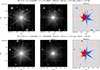 |
Fig. B.1. GTC/EMIR J-band images of the 21 targets in two epochs and the difference (red positive, blue negative). The two-epoch images are normalised and then stretched on a logarithmic scale to better visualise the faint sources around the central star. White arrow in the difference image indicates the proper motion direction of the star. For clarity, the arrow length is three times the motion during the baseline between the two epochs. All images are centred at the star position at the first epoch with an FoV of 1′ × 1′. |
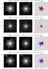 |
Fig. B.1. continued. |
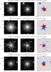 |
Fig. B.1. continued. |
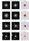 |
Fig. B.1. continued. |
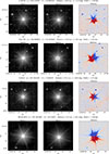 |
Fig. B.1. continued. |
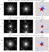 |
Fig. B.1. continued. |
All Tables
All Figures
|
Fig. 1. Top: Two epochs of GTC/EMIR J-band images of BD+02°3375 in logarithm count scale. The positions of the comoving companion candidate are pointed out by red arrows. The motion is not visible in the difference image of Fig. B.1. Bottom: Proper motion diagram of the sources. The proper motion of the primary (red cross) agrees well with Gaia (red star) within the uncertainties. The background sources extracted by daofind and by hand have almost zero proper motion (black dots). The candidate (blue cross) has a significant proper motion compared to the background sources, but is not comoving with the primary. |
| In the text | |
|
Fig. 2. Target distance histogram compared with maximum detectable distances (solid coloured lines) for different spectral types of extreme subdwarfs with low metallicities at the first-epoch GTC/EMIR J-band depth of 22.8 mag. The coloured shades indicate the uncertainty of the maximum detectable distances, which mainly result from the uncertainties of the parallax measurements. |
| In the text | |
|
Fig. 3. Explored projected physical separation ranges (au) for comoving companions of each target, with objects ordered by increasing right ascension from bottom to top. Objects with two epochs of GTC/EMIR observations are shown in orange, and the rest are plotted in blue. The black stars show the four identified known stellar companions. |
| In the text | |
|
Fig. B.1. GTC/EMIR J-band images of the 21 targets in two epochs and the difference (red positive, blue negative). The two-epoch images are normalised and then stretched on a logarithmic scale to better visualise the faint sources around the central star. White arrow in the difference image indicates the proper motion direction of the star. For clarity, the arrow length is three times the motion during the baseline between the two epochs. All images are centred at the star position at the first epoch with an FoV of 1′ × 1′. |
| In the text | |
|
Fig. B.1. continued. |
| In the text | |
|
Fig. B.1. continued. |
| In the text | |
|
Fig. B.1. continued. |
| In the text | |
|
Fig. B.1. continued. |
| In the text | |
|
Fig. B.1. continued. |
| In the text | |
Current usage metrics show cumulative count of Article Views (full-text article views including HTML views, PDF and ePub downloads, according to the available data) and Abstracts Views on Vision4Press platform.
Data correspond to usage on the plateform after 2015. The current usage metrics is available 48-96 hours after online publication and is updated daily on week days.
Initial download of the metrics may take a while.