


| Issue |
A&A
Volume 711, July 2026
|
|
|---|---|---|
| Article Number | A257 | |
| Number of page(s) | 21 | |
| Section | Planets, planetary systems, and small bodies | |
| DOI | https://doi.org/10.1051/0004-6361/202659006 | |
| Published online | 21 July 2026 | |
Next-generation Exo-REM atmospheric models Application to VHS 1256 b to emulate patchy clouds
1
LIRA, Observatoire de Paris, Univ. PSL, CNRS, Sorbonne Univ., Univ. Paris Cité,
5 place Jules Janssen,
92195
Meudon,
France
2
Laboratoire d’astrophysique de Bordeaux, Univ. Bordeaux,
CNRS, B18N, allée Geoffroy Saint-Hilaire,
33615
Pessac,
France
3
NASA-Goddard Space Flight Center,
Greenbelt,
MD
20771,
USA
4
Laboratoire J.-L. Lagrange, Université Côte d’Azur, Observatoire de la Côte d’Azur, CNRS,
06304
Nice,
France
5
IPAG, Université Grenoble-Alpes, CNRS,
38000
Grenoble,
France
6
Max-Planck-Institut für Astronomie,
Königstuhl 17,
69117
Heidelberg,
Germany
7
Fakultät für Physik, Universität Duisburg–Essen,
Lotharstraße 1,
47057
Duisburg,
Germany
8
Abteilung für Weltraumforschung und Planetologie, Physikalisches Institut, Universität Bern,
Sidlerstr. 5,
3012
Bern,
Switzerland
★ Corresponding author: This email address is being protected from spambots. You need JavaScript enabled to view it.
Received:
16
January
2026
Accepted:
21
May
2026
Abstract
Condensate clouds are a defining feature of brown dwarf and exoplanet atmospheres, producing a broad range of colours on the colour–magnitude diagram (CMD) and giving rise to spectral features such as the distinct ∼10 μm spectral imprint, a prominent diagnostic for silicate clouds. Cloud cover is likely to be heterogeneous in many objects, with observed rotational variability providing key evidence of the presence of thick and thin cloud regions rotating in and out of view. Yet current one-dimensional atmosphere models, which often lack a parameter to tune cloud optical thickness, typically fail to reproduce the spectra of highly cloudy substellar objects, especially those with complex cloud structures. Our goal is to address this limitation by upgrading the Exo-REM atmosphere model and by devising a more nuanced approach to better describe heterogeneous cloud cover with pre-computed 1D grids. Here, we present new self-consistent low- (R = 500) and medium-resolution (R = 10 000) Exo-REM grids, hereafter Exo-REM k26, featuring critical updates: (1) the incorporation of a cloud sedimentation parameter, fsed, to govern cloud opacity, thereby enabling even the reddest of objects to be accessed on a CMD and revealing a trend of decreasing fsed along the L–T transition; (2) a substantial update of the molecular opacities and abundances used, including new experimentally validated alkali line lists; and (3) the implementation of strict convergence criteria that entirely avoid unstable model solutions. Correcting an erroneous CH3D abundance leads to marked spectral changes for low-Teff (methane-rich) objects. As a consequence, applying Exo-REM k26 to the cool GJ 504 b results in a revision of its parameters (Teff = 473−12+14 K, log g = 4.0 ± 0.1 dex). For the notoriously variable VHS 1256 b, a two-column Exo-REM k26 framework that emulates cloud heterogeneities achieves a significantly improved global fit over a single 1D model. Here, a ∼ 60–40% split of thick and thin clouds best describes its atmosphere, further confirming the presence of patchy clouds. In particular, this reproduces the strong 10 μm silicate absorption in the MIRI/MRS (JWST) data of VHS 1256 b, where 1D grids had previously failed, due to the formerly unexplored low- fsed regime in the new model. The addition of the fsed dimension as well as the two-column approach for heterogeneous cloud distributions prove vital for accurately characterising cloudy sub-stellar objects.
Key words: techniques: spectroscopic / planets and satellites: atmospheres / planets and satellites: gaseous planets / infrared: planetary systems
© The Authors 2026
 Open Access article, published by EDP Sciences, under the terms of the Creative Commons Attribution License (https://creativecommons.org/licenses/by/4.0), which permits unrestricted use, distribution, and reproduction in any medium, provided the original work is properly cited.
This article is published in open access under the Subscribe to Open model. This email address is being protected from spambots. You need JavaScript enabled to view it. to support open access publication.
1 Introduction
Condensate clouds are key elements in the atmospheres of brown dwarfs (BDs; Kirkpatrick 2005; Marley & Robinson 2015) and exoplanets (Madhusudhan 2019), where they have a major impact on their emitted or transmitted spectra, and they are expected to have a pronounced effect on future reflected light observations with next-generation instruments such as the Extremely Large Telescope (ELT) and the Habitable Worlds Observatory (HWO). Changes in cloud altitude with effective temperature are generally understood to be the main drivers of spectral type and colour evolution in BDs (e.g. Cushing et al. 2008; Saumon & Marley 2008; Charnay et al. 2018): the L–T transition marks a sudden blue shift in colour over a small temperature range of a few hundred kelvin that occurs as the effective temperature decreases when silicate and iron condensate clouds begin to sink lower in the atmosphere, rendering it optically thinner at short wavelengths.
To address the challenge of modelling cloud formation and evolution, various 1D atmosphere models adopt different methodological approaches, varying in their complexity and incorporation of physical processes as well as in the range of parameters they explore. DRIFT-PHOENIX (Helling et al. 2008; Witte et al. 2009, 2011) includes a wide variety of cloud species (Fe, SiO2, TiO2, Al2O3, MgO, MgSiO3, and Mg2SiO4) in its non-equilibrium cloud model, but it does not take coagulation into account. ATMO (Tremblin et al. 2015; Phillips et al. 2020) is a cloudless model that focuses on the CO/CH4 and N2/NH3 non-equilibrium reactions that induce fingering convection, providing an alternative hypothesis for the reddening phenomenon that excludes the presence of condensate clouds. However, this approach is debated in Leconte (2018), and the assumption of cloud-free conditions has now been contradicted by many unambiguous detections of silicate cloud features (Suárez & Metchev 2022; Miles et al. 2023; Hoch et al. 2025; Mollière et al. 2025). BT-Settl (Allard et al. 2012) is a model that estimates the abundance and size distributions of cloud particles for 55 types of solids, with non-equilibrium chemistry included for several species. Lacy & Burrows (2023) incorporated disequilibrium chemistry and water clouds in their self-consistent models of Y-dwarf atmospheres. Finally, the Sonora-Diamondback model (Morley et al. 2024) belongs to the Sonora family, which also includes the Sonora-Bobcat (Marley et al. 2021), Sonora-Cholla (Karalidi et al. 2021), and Sonora Elf-Owl (Mukherjee et al. 2024; Wogan et al. 2025). It is the only Sonora model that includes clouds (following the approach in Ackerman & Marley 2001), parametrizing them by exploring their vertical extent and opacity. The ranges of parameters explored in each model are summarised in Table 1.
Our Exoplanet Radiative-convective Equilibrium Model (Exo-REM) is an atmosphere model that was initially developed to interpret upcoming photometric and spectral measurements from the new generation of instruments such as VLT/SPHERE in order to characterise the atmospheres of young Jupiters (Baudino et al. 2015). Subsequently a more elaborate self-consistent cloud model was developed (Charnay et al. 2018) that accounted for both absorption and scattering of thermal radiation. Exo-REM has since been adapted in Blain et al. (2021) for irradiated planets so as to include transmission spectroscopy. With a simple microphysics cloud model including iron and forsterite condensates, the existing Exo-REM grids manage to follow the general trend of the L–T transition on a CMD; however, the lack of a free parameter for cloud vertical distribution prevents them from reproducing the whole diversity of colours of field BDs and young giant planets (YGPs). Here, we detail the addition of a parameter designed to adjust the cloud vertical extent and opacity, namely, the sedimentation rate (fsed) parameter. This has previously been incorporated when modelling the vertical profiles of BDs and their evolution in CMDs (Ackerman & Marley 2001; Saumon & Marley 2008) but has only recently been added as an additional dimension in one other atmosphere model (Sonora-Diamondback; Morley et al. 2024).
Although the fine-tuning of condensate cloud optical thickness in atmosphere models is essential, it nonetheless assumes uniform cloud coverage over the whole surface of an object and thus does not capture the complexities of objects displaying heterogeneous distributions of clouds. Indeed, time-variations in flux have been widely observed in BDs, such as VHS 1256 b (Zhou et al. 2020) and many others (Artigau et al. 2009; Radigan et al. 2012, 2014; Metchev et al. 2015; Buenzli et al. 2015; Vos et al. 2017; Eriksson et al. 2019; Zhou et al. 2018; Bowler et al. 2020; Vos et al. 2020; Tannock et al. 2021; Vos et al. 2022; Biller et al. 2024; Nasedkin et al. 2025) as well as in planetary mass companions such as 2MASS 1207 b and 2M1207 b (Zhou et al. 2016; Adams et al. 2025), strongly suggesting the existence of large-scale atmospheric heterogeneities, most likely in the form of patchy clouds (Marley et al. 2010; Apai et al. 2013; Morley et al. 2014b). As a patchy object rotates, it would show thicker and thinner cloud zones and rapidly expose different atmospheric depths and temperatures, leading to periodic light curve variations. To corroborate these observations, global climate models (GCMs) have predicted heterogeneous cloud cover as a natural characteristic in BDs, as cloud radiative effects trigger atmospheric convection and give rise to spatial and temporal changes consistent with the variability seen across the L–T transition (Artigau 2018; McCarthy et al. 2025; Teinturier et al. 2026). While a thick zonal cloud band is predicted to populate the equator for Coriolis-dominated fast rotators, longitudinal variations are the culprits for the widely observed time variability. These could come in the shape of zonal waves, storms (Tan et al. 2025), or spots (Zhou et al. 2022) analogous to Jupiter’s Great Red Spot. However, the physical origins of such structures on directly imaged objects that have different dominating processes in their atmosphere dynamics (Tan & Showman 2017), remain elusive.
Fitting observed spectra of complex patchy objects is currently a challenge in atmospheric modelling: while standard 1D atmospheric models, with their assumption of a homogeneous atmosphere, are insufficient, sophisticated three-dimensional GCMs are computationally costly, and as it stands, creating large grids of such models aimed at fitting observations is unrealistic. Intermediate approaches consisting in combining two 1D atmospheric columns differing in cloud properties have been successfully applied in retrieval (e.g. Vos et al. 2023; Zhang et al. 2025, and Mollière et al. 2025) and forward modelling (e.g. Marley et al. 2010 and Morley et al. 2014a,b) frameworks, where in both cases the whole atmosphere was converged to a single thermal profile. Here we propose an approach consisting of combining two 1D Exo-REM k261 atmospheric columns with differing cloud optical thicknesses and thermal profiles in a forward-modelling framework to describe objects with patchy cloud cover without adding parameters to the pre-computed grid.
VHS 1256 b constitutes a prime test case for this method since time-monitoring characterises it as having one of the highest rotationally modulated variabilities of substellar objects to date. From two epochs – a 9 h HST 2018 time series (Bowler et al. 2020) and a 42 h HST 2020 time series (Zhou et al. 2022) – its peak-to-peak amplitude is estimated at 37.6 ± 2.2% at 1.27 µm. Additionally, a 38 h Spitzer/IRAC (Infrared Array Camera) observation measured a variability of 5.76 ± 0.04% at 4.5 µm (Zhou et al. 2020). The presence of thick silicate clouds was confirmed when it was observed by the JWST High Contrast Early-release Science Programme (Hinkley et al. 2022) with a combination of NIRSpec and MIRI (Miles et al. 2023), and it showed a strong characteristic silicate absorption feature in the spectrum at ∼10 µm.
Attempting to converge to a single 1D model is insufficient due to the thick patchy clouds in the atmosphere of VHS 1256 b. Petrus et al. (2024) and Lueber et al. (2024) demonstrated that none of the existing grids of pre-computed 1D models (Sonora, ATMO, Exo-REM, BT-Settl, DRIFT-PHOENIX) were able to produce an adequate fit for the JWST spectrum, most dramatically at the silicate feature. Tan et al. (2025), with their GCM, demonstrated that the complex light curve modulations of VHS 1256 b could be explained by cloud heterogeneities in the shape of a persisting dust storm; however, with their lack of disequilibrium chemistry and refined grid, they were not able to produce a satisfactory fit of the molecular absorptions in the JWST spectrum.
In Sect. 2, we present the most consequential updates to the Exo-REM model, detailing the addition of an fsed parameter, updated line lists and abundances, and the treatment of convergence issues in the code. In Sect. 3, we highlight the most notable changes in the Exo-REM spectra and use them on GJ 504 b to derive more accurate parameter values and on VHS 1256 b to stress-test the added fsed dimension while using a two-column forward-modelling approach for patchiness. In Sect. 4, we discuss the implications of the updates in Exo-REM and the limits to which we may deduce the atmospheric structure of highly cloudy objects. In Sect. 5 we summarise the work and discuss the upcoming upgrade of Exo-REM to high spectral resolution.
Comparison of substellar atmosphere model parameter ranges.
2 Model description
2.1 The radiative-convective equilibrium model: Exo-REM
Exo-REM solves for radiative-convective equilibrium, assuming that the total flux is conserved at each vertical level, the total flux being comprised of radiative and convective flux. For directly imaged objects we neglect the radiation from the exoplanet’s host star. The model is parametrized by the following input parameters: the surface gravity log g of the object (at 1 bar), its effective temperature Teff, metallicity [M/H], and the carbon-to-oxygen ratio C/O. The external structure is simply assumed to abide by the ideal gas equations, linking the pressure, density, and temperature.
An important source of opacity is the collision-induced absorption (κCIA) from H2 molecules (H2–H2) along with that of H2–He and, in some cases (high metallicity and thus H2O abundance), H2O–H2O. We modelled it using data for the three above cases from HITRAN (Karman et al. 2019). We also include Rayleigh scattering κRayleigh, although it is not a major contributor in the wavelength range modelled here (λ > 1 µm). The line absorption, κline, comes from the ro-vibrational bands originating from eleven different molecules, and the presence of resonant lines from Na and K. Finally, the last source of opacity comes from clouds of condensates (κaerosols), so that the total extinction κext can be described as the following sum:
 (1)
(1)
For the relatively cool low-mass objects (200 K < Teff < 2000 K) considered in this model, we include Nspec = 13 species (molecules and atoms) as opacity sources in κline: H2O, CH4, CO, CO2, H2S, HCN, K, Na, NH3, PH3, TiO, VO, and FeH (Table A.1 lists all isotopologues included). Their vertical volume mixing ratio (VMR) profiles are determined by calculating the chemical abundances level by level, starting from the deepest level, and moving upwards to the top of the atmosphere. Examples are shown in Fig. A.1. These profiles have 49 pressure levels with corresponding temperatures, the top of the atmosphere being the level with the lowest pressure value. Other than the Nspec species listed above, the simulated atmosphere contains only He and H2, so that, for each pressure level,  with an He/H (including hydrogen-bearing species) number ratio α = 0.0839, from the solar abundance according to Asplund et al. (2021).
2.2 Line opacities
To incorporate κline from Eq. (1) into the model, we need line opacities for each of the thirteen included species, at a range of temperatures and pressures; these can be calculated from available line lists, as provided by, for example, HiTEMP (Rothman et al. 2010), TheoReTS (Rey et al. 2016) or Exomol (Tennyson et al. 2024). A Voigt profile is assumed for the molecular lineshape up to a certain distance of line centre, beyond which a sub-Lorentzian profile is applied. The treatment of the wings for atomic resonant lines is particularly important, as it can lead to important differences in the final spectrum, as we show in the case of the alkali atoms included in the model. In addition, the isotopologue abundances must be specified in the instances where opacity data is available for several isotopologues, in which case we include them with natural abundances as listed in Asplund et al. (2021). In practice, this is done by a linear combination of the R = 106 cross-section data for each isotopologue of a molecule, weighted by their natural abundances listed in Table A.1 that we computed from Table A.2, combining them into one single cross-section file, as illustrated in Fig. A.2 for methane. This is done using Exo_k2, a python code developed to handle cross-sections and opacities (Leconte 2021).
2.2.1 Updated line lists and isotopologue abundances
Recognising a need to update certain line lists and isotopologue abundances used in Exo-REM – there being advances in their computation as well as the number of isotopologues available – we revisited them by adding all of the isotopologues for which there was available opacity data. Previously in Exo-REM, solely the main isotopologue was included for each molecule, except in the case of CH4, where 12CH4, 13 CH4, and CH3D were included, as well as the case of NH3 where 14NH3 and 15NH3 were included with a 14N/15N ratio of 500 (Blain et al. 2021; Füri & Marty 2015).
Here we have used up-to-date opacities that have been calculated, from many different sources, by Mollière et al. (2019) and can be found in the petitRADTRANS documentation3. All of the details are listed in Table A.1, and below we discuss the most notable changes.
CH4. Exo-REM already included its main isotopologue 12CH4 as well as 13CH4 and 12 CH3 D. Unlike the other two, 12CH3D is asymmetrical and has different vibration modes, with prominent band absorption at 2.7–2.9 µm, 3.2–3.4 µm, 4.25–4.66 µm, 6.5–6.9 µm, and 8.0–9.0 µm (Wilmshurst & Bernstein 1957; Rey et al. 2014). This makes it detectable and separable in spectra, and we realised that Exo-REM, despite citing a D/H ratio of 2 × 10⁻⁵ in Blain et al. (2021), included a remarkable excess of 12CH3D, leading to an over-absorption at CH3D-absorbing wavelengths. This was especially relevant for spectra at the lower range of effective temperatures, where methane is more abundant since it is more stable at low temperatures (Burrows & Sharp 1999), as it is apparent in Fig. A.1. The unweighted methane isotopologue absorption cross-sections, as well as the corrected, properly weighted (according to solar system abundances) isotopologues are shown in Fig. A.2. We therefore included the same isotopologues but with revised abundances compared to the most recent model. Figure 1 shows that this correction led to a weaker absorption in the 12CH3D-absorbing ranges.
Na and K. Since the atmospheres of giant planets and BDs are cool enough to host neutral alkali atoms, their absorption lines play a major role in shaping the observed spectra (Burrows et al. 2001, 2002; Burrows & Volobuyev 2003). The opacity in the visible and near-infrared range up to ∼1.2 μm is dominated by the heavily pressure-broadened wings of these alkali resonance lines, acting as a pseudo-continuum (Allard et al. 2003). For K I, these lines are centred at λ = 0.766 and 0.770 μm (K D2 and D1 respectively), and for Na I they are centred at λ = 0.589 and 0.590 μm (Na D2 and D1 respectively). For most self-luminous gas giants and BDs, their flux peaks close to 1 µm; this emission originates from deep layers of the photosphere, where temperatures reach 1000 K and pressures range between 10 and 100 bar. Thus, the line profile chosen for these alkalis is of utmost importance in this model as, for the Exo-REM range of temperatures for cool BDs and hot giant planet atmospheres, they appreciably dampen the flux at its peak. It has become clear that, with the alkali line wings creating absorption up to 0.4 µm from line centre, the classical adoption of a Lorentzian profile is not appropriate in simulating their absorption in He and H2-dominated atmospheres (see also Allard & Kielkopf 2025).
New ab initio calculations of the theoretical potentials for the interactions of alkali atoms with He and H2 were thus carried out in Allard et al. (2003, 2019), and validated by laboratory measurements. This motivated our decision to incorporate in Exo-REM the Na and K opacities calculated in Allard et al. (2016, 2019) respectively rather than those detailed in Burrows & Volobuyev (2003), as had been done previously. Figure 2 shows the differences in the absorption cross-section between the former and new adopted alkali profiles, with the Allard et al. (2016, 2019) profiles showing substantially more absorption at the wings. As seen in the resulting full simulated spectra in Fig. 1, the difference is non-negligible at 0.6–1.2 µm and results in a lower pseudo-continuum than previously computed for a range of effective temperatures.
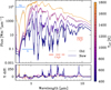 |
Fig. 1 Top panel: comparison of the new Exo-REM k26 cloudless grid (coloured) to the previous grid (in grey; Charnay et al. 2018) for models with log g = 4 dex and solar C/O and [M/H]. The difference between the two models at the same Teff is shaded. The most notable differences are due to changes in the Na and K line profiles and the revised CH3D abundance. Bottom panel : relative residual flux (Fnew − Fold)/Fold × 100. |
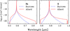 |
Fig. 2 Comparison of alkali absorption cross-sections using line lists of Allard et al. (2019) and Burrows & Volobuyev (2003) for Na (left panel) and Allard et al. (2016) and Burrows & Volobuyev (2003) for K (right panel) at P = 10 bar and T = 899.5 K, which are conditions in the atmosphere probed by the ≈ 1 μm peak flux. |
2.2.2 k-coefficients
The chemical opacities described above are, in practice, represented in Exo-REM in the form of correlated-k distributions for each species. This approach is a way of binning down high resolution cross-sections to evaluate radiative transfer at lower resolutions (Lacis & Oinas 1991). This approximation is more precise than simply binning down cross-sections to lower resolutions, and more computationally efficient than evaluating the radiative transfer, line-by-line, at the native cross-section resolution (R = 106) and subsequently binning down, as demonstrated in Leconte (2021). For the low-resolution grid, the binning down was carried out with the Python library Exo_k, which distributes the cross-section values, for each molecule, into Δν bins of a constant 20 cm−1 width, so that the resolution has a value of R = 500 at 1 μm. In each of these spectral intervals, the high-resolution cross-sections were then sorted into 16 Gauss-Legendre quadrature points, organised in order of strength of absorption, where one radiative transfer calculation is carried out for each (Baudino et al. 2015). Similarly for the medium-resolution grid, the binning down of high-resolution cross-section data was also carried out by Exo_k, but into bins of varying width so as to keep the spectral resolution constant (R = 10 000) throughout the wavelength range. At very high resolutions, the correlated-k distribution approximation is no longer numerically faster than simply computing the radiative transfer at the native resolution: computing radiative transfer at R = 70 000 for example would, with the correlated-k method, require approximately 1 120 000 calculations (70 000 × 16), while simply evaluating line-by-line at R = 106 would require 1 000 000 calculations and be more accurate (Leconte 2021). In anticipation of the subsequent upgrade of Exo-REM k2 6 to high resolutions of R = 200 000 (Radcliffe et al., in prep.), we chose here to start from high resolution crosssections, allowing us to use the same data across grids of different resolutions, so as to render them completely consistent with each other.
2.3 Cloud scheme
Clouds of condensates represent a central source of absorption in Eq. (1) when computing radiative transfer for BDs and planetary-mass companions. Clouds are governed by a balance between the downwards sedimentation of cloud particles due to gravitational settling versus the upwards turbulent mixing of condensate and vapour, as well as the evaporation of cloud particles and condensation back into clouds. We considered that at equilibrium, the upwards mixing of condensates and vapour is balanced by the downwards flow of condensate caused by sedimentation (Ackerman & Marley 2001):
 (2)
(2)
with qc and qv denoting the mass mixing ratios of condensates and vapour respectively, Kzz being the eddy diffusion coefficient and vsed the sedimentation velocity. Meanwhile, vapour condenses into clouds at supersaturation, when its pressure exceeds its saturation vapour pressure, pv > ps. The computation of mass mixing ratio of a condensate at a given level is computed by solving Eq. (2), using a formula for Kzz based on mixing length theory (Ackerman & Marley 2001), and finally the assumption that particles fall at their terminal velocity, all of which is detailed in Charnay et al. (2018). In this model we make the assumption that supersaturation is weak (meaning condensation is efficient), i.e. qv ≈ qs above cloud level, qv and qs denoting the mass mixing ratio of vapour and that at saturation respectively. We included iron (Fe) and forsterite (Mg2SiO4) clouds, using pre-computed tables of optical properties (single scattering albedo, asymmetry factor, and extinction coefficient), assuming spherical particles following a log-normal size distribution with an effective variance of 0.3, for a range of wavelengths and mean particle radii (Morley et al. 2012; Baudino et al. 2015; Blain et al. 2021). As done previously in Charnay et al. (2018), we included different ways of computing the cloud particle radii, either with a fixed sedimentation parameter or with simple microphysics. These different approaches are described in the following sections.
2.3.1 Fixed sedimentation parameter
Ackerman & Marley (2001) suggested that the vertical distribution of cloud particle radii could be simply represented by fixing the sedimentation parameter, which describes the ratio of sedimentation velocity to vertical mixing velocity and is given by
 (3)
(3)
with H being the atmospheric scale height. Fixing this in turn fixes the mean particle radius as vsed ∝ r2. Higher fsed values lead to larger mean cloud particle radii, which sediment faster and render the cloud less optically thick. The fsed value is held constant at each vertical level in the atmosphere, so that the ratio of characteristic upwards mixing timescale τmix to downwards sedimentation timescale τsed is constant. Here, we chose to fix fsed from a value of fsed = 0.5, where the clouds have almost no sedimentation, to fsed = 9, a value at which cloud particles sediment almost instantly (corresponding to an almost completely cloudless case). Large optical depths of the cloud layer significantly reduce the relatively transparent spectral windows, more noticeably in the 1–2 µm range, so that spectra with fsed = 0.5 resemble that of a blackbody, as seen in Fig. 3.
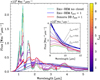 |
Fig. 3 Spectra from the R = 500 Exo-REM k26 fsed grid coming from almost cloudless cases (fsed = 9) to atmospheres with extremely optically thick clouds (fsed = 0.5). The 1–2 μm flux decreases with fsed, with the thickest cloud cover dampening spectral features the most. In red is a Sonora Diamondback model with fsed = 1, the lowest value explored in their grid; the corresponding Exo-REM k26 model is shown in blue. The other parameters are fixed at Teff = 1200 K, log g = 4.5 dex, and solar C/O and [M/H]. The 8–10 μm inset highlights which fsed values exhibit the silicate absorption. |
2.3.2 Simple microphysics: A timescale-based approach
Similar to what was done by Rossow (1978) and Cooper et al. (2003) for Earth, Mars, Venus, and Jupiter, in this approach we compare the timescales of the competing processes controlling cloud microphysics. At a given pressure, the process with the shortest timescale is said to dominate, driving particle size and thus dictating how quickly particles can grow and settle, while the other processes are neglected. The timescales associated with different processes are the following:
- (a)
Vertical mixing (τmix = H2/Kzz): This describes the time it takes for particles to be vertically moved by atmospheric turbulence over a scale height.
- (b)
Sedimentation (τsed = H/vsed): This is the time it takes for particles to fall through the scale height.
- (c)
Condensation growth (τcond): This describes the time required for a particle to grow by accreting surrounding vapor, described by the supersaturation parameter (= (qv – qs)/qs).
- (d)
Coalescence (τcoal): This is the characteristic time for particles to collide and merge during sedimentation, a process that limits the mean radius of particles by quickly removing particles larger than a certain size.
More details on this can be found in Charnay et al. (2018).
2.4 Numerical convergence
In general, to run the Exo-REM model, an initial trial pressure– temperature profile (P–T) describing the thermal structure of the atmosphere must be input, then the algorithm searches for a P–T profile that ensures conservation of flux at each pressure level. The model computes the chemistry iteratively until it converges to a radiative equilibrium solution, or until it has reached the maximum number of iterations. It is therefore necessary to input a P–T profile that is as close to the final profile as possible to minimise the number of iterations and maximise the likelihood of convergence. However, in practice, convergence does not always occur. We outline in Appendix A.3 the three markers for an ‘unconverged’ spectrum, and their treatment, allowing us to impose benchmark convergence criteria, as a fail-safe, to the Exo-REM model. Exo-REM k26 has been completely cleaned of these, leaving gaps where convergence was not achievable.
2.5 Resolution
The Exo-REM k26 low-resolution grids have a spectral resolution of R = 500 at 1 μm. However, the step size is constant in wavenumber, with Δν = 20 cm−1, meaning that the spectral resolution is not constant across wavelengths (since R = λ/Δλ), reaching values of 50 at 10 µm and as low as 2 at 250 µm. Furthermore, the binning step is also 20 cm−1, meaning that there is one point per spectral element and the binning resolution, Rb, is equal to the spectral resolution; a correct binning should be at most 1/2 of the width of the spectral bins to ensure Nyquist sampling. Therefore, the spectral resolution should be downgraded (by convolution) to R = 250 at 1 μm and so on.
Meanwhile, the Exo-REM k26 medium-resolution spectra have a true spectral resolution of 10 000: they were made by recomputing the radiative transfer at a resolution of R = 30 000 from the R = 500 chemical profiles, then subsequently downgrading the resulting spectra to a final, constant spectral resolution of R = 10000, so as to provide a super-Nyquist sampling at Rb = 30 000. This was done using Exo_k (Leconte 2021), and the same R = 106 cross-section files were used as for making the R = 500 k-tables, but this time binned down to R = 30 000 k-tables. The spectra in this medium-resolution grid, when binned down to the same resolution, are virtually identical to the corresponding R = 500 spectra, with differences in flux arising from discrepancies when evaluating radiative transfer at different resolutions.
3 Results and applications
3.1 Exo-REM k26: The new generation of models
To summarise, we therefore produced three low-resolution grids of models: one cloud-free, one with simple microphysics and lastly one with an fsed dimension spanning 0.5 ≤ fsed ≤ 9, the range of which is shown in Fig. 3. We additionally produced one new medium-resolution grid with the extra fsed dimension at a constant resolution of R = 10 000. All of these are publicly available4.
3.2 Reproducing the L–T transition
The J – K (MKO) magnitudes of spectra in the cloudless and simple microphysics grids are shown on a CMD in Fig. 4: as previously, the cloudless models do not follow the L–T transition, but instead keep steadily decreasing in J magnitude and increasing in J – K as temperature increases. Conversely, the simple microphysics models approximately follow the shift to bluer colours around Teff = 1400 K and cooler, as the forsterite and iron clouds appear and then dissipate at lower effective temperatures. While the simple microphysics grid provides a satisfactory cloud description, the grid with the added fsed dimension ensures that each and every object on the CMD is represented, even the reddest ones such as VHS 1256 b. Computing the J – K magnitudes of our model spectra for varying fsed and Teff, and interpolating onto observed L and T dwarf magnitudes (see Fig. A.3) results in a general trend along the L–T transition, whereby fsed values increase (from fsed ∼ 2.7 to ∼3.9), as shown in Fig. 5. This trend was predicted in Saumon & Marley (2008) and has been further substantiated with the X-SHYNE (X-SHooter medium-resolution near-infrared survey for Young, Nearby Exoplanet analogs) survey of 43 spectra of isolated BDs: Petrus et al. (2025) found, with Sonora Diamondback, a clear trend of increasing fsed from L1 to T7 spectral types.
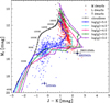 |
Fig. 4 Colour-magnitude diagram with the computed J versus J – K magnitudes for the Exo-REM k26 cloudless log g = 5 (in black) and simple cloud microphysics models (for log g = 3, 3.5, 4, 4.5, and 5 in purple, green, pink, light blue, and blue respectively) at constant solar C/O and [M/H]. The simple microphysics grid was computed with a supersaturation parameter s = 0.1. The M, L, and T dwarfs are plotted in black, red, and blue dots, respectively (Best et al. 2025). Data for GJ 504 b, VHS 1256 b, and HR 2562 b are from Kuzuhara et al. (2013), Gauza et al. (2015), and Konopacky et al. (2016), respectively. |
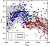 |
Fig. 5 Evolution of fsed for BDs over the L–T transition found by computing the magnitudes of Exo-REM k26 spectra of varying fsed and Teff values at log g = 4.5 and solar C/O and [M/H], then interpolating to find the fsed and Teff at the Best et al. (2025) data points. The median over 20 K Teff ranges is shown in black, and the 1σ region is shaded in grey. |
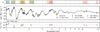 |
Fig. 6 Best fit for GJ 504 b photometry with revised parameters found with Exo-REM k26, posterior distributions of which are provided in Fig. B.4. Plotted in grey are random samples from the family of spectra with a likelihood within 1 σ of the best fit. Top panel: normalised transmission for each filter. Bottom panel: residual flux between the observed and simulated photometry. |
3.3 GJ 504 b: Impact of the CH3D correction
To exemplify the change in results brought about by the methane D/H correction in Exo-REM detailed in Sect. 2.2.1, we chose the case of GJ 504 b, a very cool object that exhibits marked methane absorption (Janson et al. 2013), and has been analysed with the previous Exo-REM grid in Mâlin et al. (2025). This faint companion was detected via direct imaging in 2011, in H-band (∼1.6 µm) Subaru/HiCIAO (the High-Contrast Instrument with Adaptive Optics) observations (Kuzuhara et al. 2013), at a wide orbit with a projected distance of 43.5 au around GJ 504 A. The primary had been observed in the course of the SEEDS (Strategic Explorations of Exoplanets and Disks with Subaru) survey at a distance of 17.56 ± 0.08 pc, and reported to be a Sun-like main sequence star of spectral type G, with a mass of M* = 1.2 M⊙ and rather young age of  Myr based on stellar gyrochronological and chromospheric activities (Kuzuhara et al. 2013). However, this was debated by Fuhrmann & Chini (2015) and D’Orazi et al. (2017), who suggested an older stellar age, ranging from 1.5 to 4 Gyr. They proposed that the high levels of rotation and chromospheric activity, typically indicative of a young stellar age, could result from the recent engulfment of a short-period hot Jupiter, which supported the argument for an older system. Finally, the most recent isochronal studies suggest that the star may either lie above the main sequence on the Hertzsprung–Russell diagram and thus have an age of 4.0 ± 1.8 Gyr or be much younger, with an age of 21 ± 2 Myr (Bonnefoy et al. 2018).
Naturally, this degeneracy in age transfers to its companion GJ 504 b, and gives rise to two distinctly different values for its mass. For the observed flux, it would have to be a relatively young gas giant or a much older BD: using the hot-start model from Baraffe et al. (2002) with an age of  Myr (Kuzuhara et al. 2013) leads to a mass of M =
  MJup, while taking the isochronal ages of 21 ± 2Myr and 4.0 ± 1.8 Gyr from Bonnefoy et al. (2018) would yield mass values of M =
  MJup or M =
  MJup respectively. GJ 504b exhibits notable differences compared to previously observed exoplanets, displaying a bluer colour (J – H = −0.23 mag; Kuzuhara et al. 2013) and being one of the coolest companions ever observed directly, with an effective temperature of ∼500 K (Mâlin et al. 2025). This, along with its discrepancy in age and mass, is a powerful incentive for further investigation of GJ 504 b and how it formed.
We conducted forward modelling with the low-resolution Exo-REM k26 grid using ForMoSA5 (Petrus et al. 2023), a Bayesian forward-modelling tool that uses a nested sampling algorithm for parameter exploration with a given likelihood, as done for example in Petrus et al. (2021, 2023) or Palma-Bifani et al. (2023, 2024). We used 4000 live points and uniform priors spanning the whole parameter space. We included the J2, K2, and CH4L photometry 3σ upper limits of by adding a component to the total χ2 in the likelihood function: considering a non-detection of flux FUL = μnoise + 3σUL with an average, μnoise = 0, and dispersion σUL for each upper limit filter, we used a cumulative distribution function to contribute to the total χ2 when the model flux approaches the upper limit from below, or lies anywhere above, similarly to Sawicki (2012). The total goodness-of-fit is

where Φ(·) denotes the standard normal cumulative distribution function. Figure B.4 shows the resulting posterior distributions. We obtained an effective temperature of Teff = 473−12 K, a surface gravity of log g = 4.0 ± 0.1, a radius of R =  RJup, a metallicity of [M/H] = 0.9 ± 0.1 dex, a carbon to oxygen of C/O =
  , and fsed of
  , as shown in Fig. 6 and summarised in Table 2, corresponding to a χ2red = 1.38. This yielded an inferred luminosity of log L/L⊙ = −6.19 ± 0.02 and mass of M =
  MJup respectively. The mass that we found is in accordance with the age of
  Myr from Kuzuhara et al. (2013). However, there are biases in purely atmospheric forward modelling analyses for mass determination; we have not coupled the model with an interior or thermal evolution model, so we cannot completely exclude the other possible ages (and thus masses).
3.4 VHS 1256 b: A temperamental companion
Displaying strong observational pointers towards thick, patchy silicate cloud cover, the elusive VHS 1256 b presents an excellent case to stress-test the medium-resolution Exo-REM k26 models, with their wide range of fsed values. It was discovered using the VISTA Hemisphere Survey (Gauza et al. 2015) around the M dwarf binary VHS J125601.92–125723.9 at a projected separation of 105 au (Gauza et al. 2015; Rich et al. 2016; Stone et al. 2016).
Originally, the host star was thought to be a single M dwarf (and not yet known to be a binary), and a distance measurement of d = 12.7 ± 1.0 pc was initially determined by Gauza et al. (2015), which suggested a planetary mass of M = 11−20 MJup for the companion. However, once the star was found to be an equal-mass binary, the original distance measurement severely conflicted with the expected luminosities of the host star components, and the spectrophotometric distance of d = 17.2 ± 2.6 pc was found by Stone et al. (2016). This was definitively resolved by high-precision astrometry from Dupuy et al. (2020) with the Canada-France-Hawaii Telescope, which yielded a revised distance measurement of d =  pc. This dramatically increased the expected intrinsic luminosity and thus – through the Saumon & Marley (2008) evolution model – the mass, effective temperature, and surface gravity to M = 19 ± 5 MJup, 1240 ± 50 K, and
  dex, respectively, placing it in the BD mass realm. Recently, Dupuy et al. (2023) derived an age of 140 ± 20 Myr for the system using the Baraffe et al. (2015) evolutionary model; with VHS 1256 b’s observed luminosity, this places it in a region of overlap between deuterium-inert and deuterium-fusing evolutionary model tracks from Saumon & Marley (2008). This thus yields two possible masses of M = 12.0 ± 0.1 Mjup and 16 ± 1 MJup, corresponding to a deuterium-bearing or deuterium-depleted object respectively. The lower-mass scenario would have a corresponding R = 1.3RJup, Teff = 115 3 ± 5, and log g = 4.268 ± 0.006, while the higher-mass scenario would correspond to R = 1.22RJup, Teff = 1194 ± 9, and log g = 4.45 ± 0.03 (Dupuy et al. 2023). Through light curve fitting from 36-h Spitzer/IRAC monitoring, this companion has been attributed a rotational period of P = 22.04 ± 0.05 h (Zhou et al. 2020), the upper limit of BD rotation periods. Poon et al. (2024) found a line-of-sight spin axis inclination of ip = 90 ± 18°, meaning that the viewing geometry is close to edge-on.
VHS 1256 b exhibits clear signs of vigorous atmospheric dynamics. It is the most variable object observed to date, shows a shallow L-band methane absorption indicative of disequilibrium chemistry (Miles et al. 2018), has an extremely red J - Ks colour of 2.47 mag (see our Fig. 4; Gauza et al. 2015), and displays pronounced silicate absorption – together, these features point to intense vertical mixing and an optically thick, patchy photospheric cloud cover (Madhusudhan et al. 2011; Marley et al. 2012). As evidenced by Petrus et al. (2024) and Lueber et al. (2024), the existing 1D pre-computed models have difficulties in recreating the multifaceted structure and dynamics of VHS 1256 b’s atmosphere, and most strikingly do not reproduce the silicate absorption. To show this particular spectral feature, models necessitate optically thick cloud cover, a condition that can be produced by a low fsed regime. This constitutes the motivation for an application of our new models, that do indeed explore these low values, on VHS 1256 b.
Best-fit parameter values for the GJ 504b photometry using the former version of Exo-REM versus using Exo-REM k26.
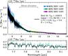 |
Fig. 7 Top panel: one-column best fit in black for only the VHS 1256 b MIRI/MRS data (Gauza et al. 2015) from forward modelling with the medium resolution Exo-REM k26 grid. Observation data are coloured according to MIRI channels. Bottom panel: zoom in on the best fit. The 1σ uncertainty is shown in grey in the top panel, and in the bottom panel, it is shown as grey error bars for one out of four points. |
3.4.1 Classical approach
We performed forward modelling using ForMoSA taking the medium resolution Exo-REM k26 models in tandem with the MIRI/MRS spectrum from Gauza et al. (2015), setting 500 living points with flat priors exploring the entire parameter space. The corresponding best fit and posterior distributions are shown in Fig. 7 and Fig. B.1 respectively; in particular we were able to reproduce the silicate absorption with, as expected, a low fsed value of 0.82, as well as a super-solar metallicity and a Teff of 1038 K, a temperature lower than previous estimates. With  , the overall shape of the pseudo-continuum is a good fit and the absorption features match up, but do not completely reflect the depth that is seen in the observations.
To test a broader range of wavelengths, we ran ForMoSA in the same conditions, but also included the JWST/NIRSpec portion of the spectrum, so that the fitting spanned from 1 to 18 µm. The best-fit model for NIRSpec + MIRI/MRS data is shown in Fig. 8, with posterior distributions in Fig. B.2 corresponding to Teff = 1032 K, a much lower metallicity, and an overall fsed = 1.2. This model does not show a pronounced silicate dip, but does nevertheless fit closer, with  , than any attempted fitting with the previous Exo-REM or current ATMO, BT-Settl, DRIFT-PHOENIX, and SONORA Diamondback model grids, which had
  , 334, 673, 301, and 522, respectively (Petrus et al. 2024). It should be noted that the best-fit model previously obtained for only the MIRI data, shown in grey in Fig. 8, clearly fails to fit the lower wavelengths of the NIRSpec data. We found that the silicate feature could only begin to be accessed with fsed < 1, but that the general disk averaged shape of the VHS 1256 b JWST spectrum resembled one of fsed > 1. This underscores the limitations of 1D models: the variability monitoring of VHS 1256 b strongly indicates heterogeneous cloud cover, which cannot be adequately described by a single 1D spectrum, with its limiting assumption of atmospheric homogeneity.
3.4.2 A two-column approach
To attempt a non-homogeneous description of VHS 1256 b’s atmosphere, we suggested that multiple Exo-REM k26 models of different fsed values would together imitate a patchy cloud cover scenario, in a ‘1D+1D’ manner, similarly to Vos et al. (2023), Zhang et al. (2025), Mollière et al. (2025), Marley et al. (2010), and Morley et al. (2014a,b), the differences being discussed in Sect. 4.4. A two-column approach was proposed for VHS 1256 b in Miles et al. (2023) using PICASSO 3.0 (Mukherjee et al. 2023), precomputing an fsed = 0.6 and fsed = 1.0 model separately, then manually combining them linearly with a 90–10% split, but the authors were not able to produce a satisfactory fit or reproduce the silicate cloud feature. We applied a similar approach but, by contrast, in a forward modelling framework, with pre-computed grids of self-consistent models, where each iteration explores a linear combination of two different models with common Teff, C/O, [M/H], and log g, allowing only fsed to vary between both spectra. An α parameter (0 ≤ α ≤ 1) was added to allow the proportions of each fsed model to vary and thus alter the percentage of thick cloud coverage:
 (4)
(4)
Each of the two columns has its own self-consistent thermal profile at radiative-convective equilibrium. We re-ran ForMoSA in these conditions with the whole JWST spectrum, which took ∼88 h to converge on seven processors. The resulting posterior distributions are shown in Fig. B.3. The condition fsed, 1 < fsed, 2 was imposed to avoid two identical solutions. The resulting best fit ( ) yielded a common Teff = 1153 K, log g = 4.0 dex, [M/H] = 0.08 dex, C/O = 0.60, and R = 1.2 RJup, with an α = 0.62 for fsed, 1 = 0.7 and fsed, 2 = 2.4, and is shown in Figs. 9 and 10. A summary of the retrieved best-fit parameters is shown in Table 3, and a discussion on the misrepresentative nature of the narrow error bars on the posterior distributions found when forward modelling with the VHS 1256 b JWST data can be found in Appendix B.1. Our retrieved Teff and radius are consistent with the values found in Dupuy et al. (2023) for their lower-mass solution (12.0 ± 0.1 MJup). The mass value obtained from our retrieved log g and radius (M = 5.8 MJup) differs from this, but given the uncertainty associated with mass retrieval by both atmospheric models (primarily related to gravity determination; see Petrus et al. 2023) and evolutionary models (arising from assumptions regarding clouds, thermal structure, core composition, and initial conditions), our value remains reasonably in accordance with Dupuy et al. (2023). Together, these mass estimates point towards VHS 1256 b being a planetary-mass object.
The molecular absorptions are well fitted owing to the fsed = 2.4 emission, while the silicate band is also adequately represented owing to the fsed = 0.7 model which produces the necessary condition for silicate absorption at 10 µm. As seen in Fig. 11, the low fsed silicate cloud deck sits at higher altitudes (and therefore the τcloud = 1 level) than the so-called photosphere, while the higher fsed column has a thinner and lower-altitude cloud layer and thus a deeper τcloud = 1 level. Figure 12 shows that, as a result, the overall absorption in the fsed = 0.7 column is dominated by clouds, leading to the outgoing flux emanating mostly from the cloud top at higher altitude, while the thin cloud coverage column radiates flux that is shaped by gas absorption in higher atmospheric layers than its thin cloud deck. The atmosphere in the fsed = 0.7 column has a higher temperature than the former, owing to greenhouse effects, meaning that, although both Teff values are the same, the overall temperature profile for fsed = 0.7 is shifted by ~500 K underneath the cloud deck of that column.
In both Figs. 8 and 9, a small but distinct peak is apparent in the residuals at ∼4.3 µm, corresponding to an over-absorption in the model. This discrepancy is due to an excess of phosphine as a consequence of an incomplete understanding of the phosphorous chemistry (e.g., Leggett et al. 2021).
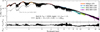 |
Fig. 8 Top panel: same as Fig. 7 but with the MIRI + NIRSpec VHS 1256 b observations (Gauza et al. 2015). The best fit for the MIRI/MRS spectrum only from Fig. 7 is shown in grey, with reduced resolution for visibility. Bottom panel: residual flux divided by the simulated flux. |
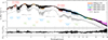 |
Fig. 9 Final best fit for VHS 1256 b. Top panel : same as Fig. 8 but using the two-column approach. Best-fit parameters are Teff = 1153 K, log g = 4.0 dex, [M/H] = 0.08 dex, C/O = 0.60, and R = 1.2 RJup, with an α = 0.62, so a linear combination of fsed = 0.7 (62%), shown with a grey dashed and fsed = 2.4 (38%) a grey solid line. Both grey fsed components have been scaled by their proportion and multiplied by a factor of 0.6 for visibility. The two fsed component spectra are shown with reduced resolution for visibility. Bottom panel: same as Fig. 8. |
Retrieved atmospheric parameters for the JWST VHS 1256 b data.
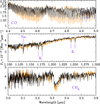 |
Fig. 10 Zoom in on the final two-column best-fit model (black) and observation (orange) of VHS 1256 b showing, from top to bottom, primarily the CO, alkali, and CH4 absorptions. |
4 Discussion
4.1 Implications for GJ 504b and low-temperature objects
The correction of the faulty D/H ratio for methane that had been applied in the previous Exo-REM grid resulted in an appreciable revision of the derived parameters for GJ 504 b. The Mâlin et al. (2025) study, that used the previous Exo-REM grid and the same photometry, reported a higher effective temperature of Teff =  K and a lower surface gravity of log g =
  compared to our revised Teff = 473−12 K and log g = 4.0 ± 0.1 (see Table 2). Critically, our higher surface gravity is more consistent with evolutionary models for its luminosity, resulting in a derived mass of M = 6.0−1′3 MJup and firmly placing GJ 504 b in the younger planetary-mass regime. This finding, with the enriched C/O and [M/H], supports scenarios of planetary formation (e.g. core accretion) for this wide-orbit companion, contrasting with dynamical instability or gravitational fragmentation scenarios often invoked for BDs (Pollack et al. 1996). The magnitude of this parameter change highlights that the previous overabundance of CH3D in Exo-REM biased the retrieved effective temperature and surface gravity for all Teff ≲ 700 K objects, where methane is highly abundant. We strongly recommend that all low-Teff objects previously analysed at methane-absorbing wavelengths using the older Exo-REM grids be re-evaluated.
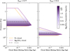 |
Fig. 11 Vertical cloud structure for both fsed columns used to describe the patchy cloud cover of VHS 1256 b. We show the cumulative forsterite (Mg2SiO4) cloud opacity (from the top layer) at λ = 1 μm and the pressure level corresponding to a cloud opacity of τ = 1 (dashed). |
4.2 The critical role of cloud thickness parametrisation
The case of VHS 1256 b brings into sharp perspective the need for a dimension geared at tuning cloud particle radii in substellar atmosphere grids, such as the fsed parameter which was added to Exo-REM. Grids relying on fixed cloud profiles or simple microphysics often fail to follow the overall shape of observed spectra or access spectral features induced by highly optically thick clouds, such as the strong 10-µm silicate absorption observed in VHS 1256 b and many other objects. We have demonstrated here that this feature can be accessed with Exo-REM k26 models with a very low cloud sedimentation parameter fsed < 0.7. A low fsed ensures that the cloud layer remains suspended above the photosphere (τ ≈ 1 surface), allowing the cloud opacity (τcloud) to dominate over the gas opacity and thus giving rise to the necessary condition for silicate absorption. No other models have explored this low- fsed regime yet. While the SONORA-Diamondback model includes fsed parametrization, it does not extend to the extremely low values required to fully fit the silicate absorption in highly cloudy objects such as VHS 1256 b, as evidenced by Fig. 3. Furthermore, the fsed parameter allowed us to cover all objects on the CMD, no matter how red: simple microphysics follows the general trend in the L–T transition, but fails to represent the cloudiest of atmospheres. Our results suggest that fsed could vary on BDs along the L–T transition, with the coolest L-dwarfs having low fsed’s, and warmest T-dwarfs having the higher fsed’s. A large-scale statistical analysis of fsed values of BDs along the L–T transition derived through forward modelling could further confirm, and perhaps explain the mechanisms behind this behaviour.
 |
Fig. 12 Left panel: photospheric pressures, from where most of the thermal emission originates, for both components (atmosphere columns) of the spectrum of VHS 1256 b. The colour indicates the temperature at the respective pressure. Right panel: P–T profile for the fsed = 0.7 (red) and 2.4 (blue) column. |
4.3 Towards the mapping of clouds on VHS 1256 b
Here we have shown that, with grids of pre-computed 1D models, one can nevertheless move towards a more complex description of objects with heterogeneous cloud cover. The relative success of the two-column model for VHS 1256 b further confirms that its atmosphere is better described as two distinct zones of differing cloud opacity, rather than one single homogeneous cloud coverage. Furthermore, with the lower fsed exploration of Exo-REM k26 and forward modelling framework, we managed to reproduce the silicate feature while fitting the overall spectrum and molecular absorptions (Fig. 10).
With the two-column approach we can attempt to constrain thick-thin cloud surface fraction on patchy objects (here, the α parameter), provided that the viewing angle is constrained – an equator-on view is favourable and more representative of the entire object’s surface since variations are largely latitudinal (Teinturier et al. 2026). For VHS 1256 b, the α value we find implies a combination of 62% thick cloud coverage of fsed = 0.7, along with 38% thinner cloud coverage of fsed = 2.4, coherent with the large surface area of observable cloud expected for the equator-on view of this companion: the fraction we find seems qualitatively consistent with the GCM results in Teinturier et al. (2026) for a Teff = 1000 K brown dwarf, that predict a thick cloud belt at the equator. A possible configuration for this result is shown in Fig. 13, with a cloud belt of fsed = 0.7 as well as spots and zonal waves that could cause the elevated rotationally modulated variability observed for VHS 1256 b. However, the α we find, in reality, only represents the proportions of the faces visible throughout the JWST observations. We expect the proportion of thick cloud coverage to change with time, causing the observed variability on VHS 1256 b.
Taking the simplistic solution where the object is strictly populated by the fsed regimes (fsed = 0.7 and 2.4), we can obtain a schematic view of how much the proportions of thick-to-thin cloud cover, α, would need to change from one face of VHS 1256 b to the opposite, one face producing the minimum of the observed light curve and vice-versa (each with an associated αmin and αmax respectively). This gives us an order of magnitude of how much patchy cloud cover has structures that vary longitudinally. To do so, we compute the flux contrast between the two theoretical cloud regimes at the observationally time-resolved wavelengths and compare it to the actual observed amplitude in the light curve over a period of rotation.
For example, at the HST observation wavelength (1.27 µm), the two thick-thin cloud spectra proposed here for VHS 1256 b have a flux of 3.1 × 10⁻¹⁶ and 7.8 × 10⁻¹⁶ W m−2 μm−1 respectively. This would produce a 96% variation from the average disk-integrated flux at 1.27 µm between faces over one rotation, if each hemisphere were completely populated by only thick or thin cloud coverage (so α = 0 then α = 1 half a rotation later; 100% of the surface changing in fsed value). From fitting the 2020 HST light curve though, the object exhibits, over 1 rotation, an actual peak-to-peak amplitude of 24.7% at 1.27 µm (Bowler et al. 2020), which requires that only a subset of the surface varies in fsed value from one face to the other. Using this and the flux contrast between the two cloud components at 1.27 µm, we infer that a change of 25% of the visible surface is sufficient to reproduce the HST observed modulation (so an α change of Δα = 0.25). With the assumption that the α = 0.62 we find in our two-column best fit lies at the average flux of the light curve at this wavelength, this corresponds to a thick cloud coverage changing from αthick = 0.50 at the maximum to αthick = 0.75 at the minimum flux on the HST light curve.
With the same logic applied on the Spitzer observation of 5.76% variation over a period at 4.5µm (Zhou et al. 2020), we deduce a fraction of 6 % longitudinal patchiness, so an alpha varying by Δα = 0.06 between the face producing the maximum and that producing the minimum. The full calculations are detailed in Appendix C). The Δα values found at each wavelength are different, reflecting the overly-simplistic nature of this analysis – while the two fsed regimes we find produce a good fit to the spectrum, they can only go so far when describing the highly complex 3D dynamics of VHS 1256 b (see the discussion in Sect. 4.4). Furthermore, when attempting to constrain the cloud configuration of intensely variable objects, a huge caveat can lie in the nature of the observations themselves: in the test case of VHS 1256 b we have fitted the combined NIRSpec and MIRI spectrum as a single, instantaneous snapshot. However, VHS 1256 b has a rotational period of ∼22 hours, and is dramatically time-variable (the order of magnitude is shown as red error bars on Fig. 9). Given the time elapsed between the NIRSpec and MIRI observations, it completed a significant fraction of its rotation, meaning that the observed surface, and thus the overall cloud fraction, α, likely varied temporarily during the measurement – we fitted a time-averaged spectrum with a single α fraction that would in fact be changing as the planet rotates. This introduces additional sources of uncertainties that are not taken into account in the fit and highlights that our two-column solution, while highly successful spatially, cannot account for the full spatio-temporal dynamics of the atmosphere.
With a simple two-column approach, we derived the rough proportions, thickness, and even variation of cloud coverage with time, but we could not constrain the shape, nature, and exact distribution of the structures on VHS 1256 b. The HST light curve has complex variations, and Zhou et al. (2022), thanks to light curve fitting, show that it is best represented by three sinusoidal components with periods of ∼19, 15, and 10.5 h, suggesting multiple spots and waves modulating the variability, each with much smaller peak-to-peak amplitudes than that found by Bowler et al. (2020). Tan et al. (2025), with their GCM, found that the heterogeneities on VHS 1256 b could come primarily in the form of a complex massive planetary-scale silicate and iron dust storm creating cloud radiative feedback, rotating eastwards in and out of view. However, their lack of disequilibrium chemistry is a limitation, and, with our inclusion of disequillibrium chemistry and finer grid, which is more computationally achievable for 1D models, we obtain a substantially closer fit of the spectral features on the JWST spectrum, in particular for the CO, H2O, and CH4 bands, as Fig. 10 shows.
Multi-wavelength time-resolved monitoring is the most effective pathway to constraining the full 3D heterogeneous structure of sub-stellar objects, and obtaining more for VHS 1256 b will be decisive in corroborating or correcting any of the preliminary theories put forward here regarding its atmospheric configuration. To further constrain the vertical structure of clouds on VHS 1256 b, we necessitate time-resolved monitoring at adjacent wavelengths: since different wavelengths probe distinct atmospheric heights, if the modulation is weaker at the wavelength probing the higher atmosphere compared to the modulation of the latter, this could indicate an intermediate cloud deck between both layers. The modulations can be directly compared if the two wavelengths probed are closeby and thus have almost identical cloud optical properties and Planck functions (Zhou et al. 2020), such as the 1.4 µm continuum region with its adjacent water absorption that probes much higher altitudes. From our analysis, we would expect an anti-correlation between simultaneous observations at 1.27 and 4.5 µm, with the flux being higher in the thinner cloud zone at 1.27 µm and the opposite at 4.5 µm. Simultaneous time-resolved monitoring at these wavelengths will be decisive in further refining our knowledge of VHS 1256 b.
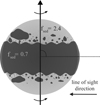 |
Fig. 13 Simplified schematic of a possible cloud configuration of VHS 1256 b at the time the JWST observations were recorded. Here we show a physically plausible configuration of waves and spots that could cause the complex sinusoidal rotationally modulated variations reported in Zhou et al. (2022). The fsed = 0.7 region would emanate flux from higher altitude and give rise to silicate absorption, while the fsed = 2.4 region would emanate from lower regions, shaping predominantly the shorter wavelengths of the spectrum. |
4.4 Advantages and limitations of the two-column approach
The two-column approach allows for a non-homogeneous description of atmospheres in cases where patchy cloud cover is strongly suspected, and where, as a result, a single 1D model does not fit. This constitutes an excellent intermediate approach from GCMs which are time-consuming and, as it stands, cannot be generated for each object or made into large grids geared at closely fitting any observation. However, this approach entails making extreme simplifications.
An assumption made is that the atmosphere is described only by two distinct vertical cloud distributions, with a sharp transition from thicker to thinner cloud zones rather than the predicted (albeit steep) gradient from thinner to thicker cloud cover shown in GCMs (Teinturier et al. 2026). Since our methodology adopts individual thermal profiles for each of the two atmospheric columns, it implicitly assumes no horizontal heat redistribution between them; at the other extreme, other studies (e.g. Marley et al. 2010; Morley et al. 2014b; Mollière et al. 2025) converge to a single thermal profile for the entire atmosphere, thereby implying complete heat redistribution. In reality, an intermediate regime is expected, in which the degree of heat redistribution is governed by the competition between radiative cooling timescales and dynamical transport timescales. In the deep atmosphere, at pressures exceeding ∼106 Pa, the horizontal advective timescale is expected to be shorter than the radiative timescale, resulting in efficient thermal homogenisation and similar temperature structures between cloudy and non-cloudy regions. At lower pressures, however, the radiative timescale decreases rapidly and becomes shorter than horizontal advective timescales, allowing local radiative equilibrium to dominate and thermal contrasts to persist between regions of differing cloud opacity (Seager & Deming 2010). We note that Zhang et al. (2025) explored atmospheric retrievals combining patchy clouds and distinct thermal profiles between the two columns, enforcing convergence of both profiles in the deep atmosphere (>106 Pa) while allowing differences at lower pressures. The atmospheric layers probed by the VHS 1256 b spectrum (∼103−105 Pa) lie firmly within the latter (lower-pressure) regime; using τadv = Rp/v with Rp the planet radius and v the horizontal wind speed (∼ 100m s−1; Teinturier et al. 2026), and τrad = Pcp/4gσT3 with P, T, cp, g and σ the pressure, temperature, specific heat capacity, gravity, and Stefan-Boltzmann constant, we find τrad ~ 3 × 10⁴ s and τadv ~7 × 10⁵ s, so τrad ≪ τadv. Therefore, at these pressures, horizontal heat redistribution is weak and a distinct temperature difference (of ∼300 K) between cloudy and cloud-free zones is predicted by the GCM presented by Teinturier et al. (2026).
However, our thick- and thin-cloud thermal profiles in Fig. 12 exhibit a more pronounced divergence (∼500 K) within the layers probed by the observations. It is improbable that this temperature contrast could physically be maintained between the centres of thick and thin cloud zones at these pressures; this is a major limitation in our method. The vast thermal contrast we find would likely be reduced if the effective temperatures between both zones were also allowed to vary, a physical attribute demonstrated by GCM studies, which showed an expected difference in outgoing longwave radiation between cloudy and non-cloudy zones owing to the reduction of emergent flux from thicker cloud layers. However this entails adding a dimension to the forward modelling analysis that is already time-consuming due to the high-resolution and expanse of the JWST data used here. An addition to our framework whereby temperature contrasts beyond a certain point are forbidden could address the problem of large thermal contrast but would require a physically motivated threshold of temperature difference. Although Teinturier et al. (2026) predicted a value, a discrepancy also arises from the fact that their GCM is computed under different conditions and without the inclusion of iron clouds, which are expected to be present at these temperatures and would enhance the greenhouse effect, increase local radiative timescales, and thus exacerbate temperature contrasts between cloudy and non-cloudy regions. They also adopted log g = 5 dex and a 5 h rotation period. VHS 1256 b, with its slow rotation coupled with unusually high variability, is expected to display substantially different atmospheric dynamics.
The Exo-REM model has the functionality of simulating patchy clouds, similarly to Marley et al. (2010), as a linear combination of a cloudless and cloudy column and evaluating the radiative transfer with one single thermal profile. However, doing so would lead to an additional dimension (cloud fraction) to the computed grid of models, and would require choosing one fsed value for each column, thus oversimplifying the cloudy scheme. Instead, the approach chosen here allows for any combination of fsed instead of assuming completely cloudy and cloudless patches. On the other hand, two-column retrieval frameworks require on-the-fly calculations of both atmospheric chemistry and radiative transfer, enabling a highly flexible, data-driven exploration of cloud properties. Such an approach allows for fine-tuning across a wide range of cloud parameters, including fsed, Kzz, particle size distributions, and cloud mass fractions at the base of the cloud deck. Applying a similar retrieval framework to VHS 1256 b, in which multiple silicate cloud species are explored, could plausibly yield an even closer match to the observed 10 µm feature (Hoch et al. 2025). The forward-modelling approach adopted here, however, relies exclusively on pre-computed grids of atmospheric models and is therefore considerably less computationally demanding; in fact many retrieval analyses, due to their high numeral cost, are constrained to downgrading the observation resolution (e.g. by Zhang et al. 2025), thus losing precious spectral information.
Rather than aiming to recover a fully self-consistent and physically accurate description of the atmosphere, our objective is to demonstrate that combining multiple 1D atmospheric columns with differing cloud properties provides a practical and physically motivated step towards capturing the spectral complexity of patchy atmospheres. This approach enables a more nuanced representation of cloud heterogeneity than a single 1D model, while avoiding the need to run sophisticated GCMs, perform on-the-fly radiative transfer, or introduce additional dimensions into already memory-intensive model grids.
5 Conclusions
We have taken measures towards obtaining a more nuanced and complex description of the atmospheres of substellar objects when using pre-computed 1D models, focusing in particular on the modelling of their cloud coverage. To this end, we did the following:
We generated a new, coherent set of self-consistent Exo-REM atmosphere models (at R = 500 and R = 10 000), titled ExoREM k26, with updated molecular opacities, most notably changing the alkali line profiles for experimentally validated broader line wings. Critically, the implementation of robust numerical convergence criteria ensures the final grids are free from the unphysical, numerically unstable spectra that were plaguing the previous Exo-REM grid (Charnay et al. 2018);
We corrected the CH3D overabundance in the previous grid, which resulted in an appreciable revision of the derived parameters for GJ 504 b and yielded a lower effective temperature (ΔTeff = 39 K; —3σ) of Teff =
 K and a higher surface gravity (Δ log g = 0.55; ~+7σ) of log g = 4.0 ± 0.1 dex than in the previous study using Exo-REM with the same data (Mâlin et al. 2025). This finding places the companion firmly in the young, planetary-mass regime (M =
  MJup). A re-evaluation of all low-temperature objects previously modelled with the older Exo-REM grid is advised;
We included the sedimentation parameter, ranging from 0.5 ≤ fsed ≤ 9, which proved essential for modelling the extreme range of cloud opacities in substellar atmospheres. We demonstrated that low fsed values (< 1) are necessary to access the strong silicate absorption characteristic of highly optically thick clouds, a regime not fully explored by previous models. We confirm that fsed must evolve, increasing across the L–T transition to explain the sinking cloud deck;
We introduced and applied a two-column forward modelling scheme for pre-computed grids of self-consistent 1D models, which emulates cloud patchiness by linearly combining two self-consistent atmosphere columns differing in cloud optical thickness and thermal profiles. This simplistic approach constitutes a vast improvement from using singular 1D models on patchy objects whilst also bypassing the need to add dimensions to pre-computed grids or to run computationally costly retrievals or GCMs;
We have proposed a patchy cloud configuration for VHS 1256 b with the two-column approach that considerably improves the fit of the full JWST spectrum compared to the classical 1D approach. The best-fit model sums a 62% thick cloud component (fsed = 0.7) and a 38% thin cloud component (fsed = 2.4), with the strong silicate absorption being produced by the high altitude and opacity of the low-fsed column. The derived bulk parameters are Teff = 1153 K, log g = 4.0 dex, [M/H] = 0.08 dex, and C/O = 0.60.
This work establishes the next generation of Exo-REM grids as representing a robust and accessible framework for interpreting directly-imaged brown dwarf and giant planet photometry and spectroscopy. A high-resolution Exo-REM k26 grid6 (R = 200 000) spanning 0.9–6.0 µm necessary for detailed chemical and kinematic studies from high-resolution spectrographs (e.g. VLT/CRIRES+, VLT/HiRISE) is already available and will be presented in an upcoming publication (Radcliffe et al., in prep.).
Acknowledgements
This project has received funding from the European Research Council (ERC) under the European Union’s Horizon 2020 research and innovation programme (COBREX; grant agreement No. 885593). This work was granted access to the HPC resources of MesoPSL, financed by the Île-de-France Region and the Equip@Meso project (reference ANR-10-EQPX-29-01) of the Investisse-ments d’Avenir programme supervised by the Agence Nationale pour la Recherche. S.P. was supported by an appointment to the NASA Postdoctoral Program at the NASA-Goddard Space Flight Center, administered by Oak Ridge Associated Universities under contract with NASA. G.-D.M. acknowledges the partial support of the Deutsche Forschungsgemeinschaft (DFG) through grant MA 9185/2-1.
References
- Ackerman, A. S., & Marley, M. S. 2001, ApJ, 556, 872 [Google Scholar]
- Adams, A. D., Zhou, Y., Marleau, G.-D., et al. 2025, AJ, 170, 289 [Google Scholar]
- Allard, N. F., & Kielkopf, J. F. 2025, A&A, 703, A71 [NASA ADS] [CrossRef] [EDP Sciences] [Google Scholar]
- Allard, N. F., Allard, F., Hauschildt, P. H., Kielkopf, J. F., & Machin, L. 2003, A&A, 411, L473 [NASA ADS] [CrossRef] [EDP Sciences] [Google Scholar]
- Allard, F., Homeier, D., & Freytag, B. 2012, Phil. Trans. R. Soc. A, 370, 2765 [CrossRef] [PubMed] [Google Scholar]
- Allard, N. F., Spiegelman, F., & Kielkopf, J. F. 2016, A&A, 589, A21 [NASA ADS] [CrossRef] [EDP Sciences] [Google Scholar]
- Allard, N. F., Spiegelman, F., Leininger, T., & Mollière, P. 2019, A&A, 628, A120 [NASA ADS] [CrossRef] [EDP Sciences] [Google Scholar]
- Apai, D., Radigan, J., Buenzli, E., et al. 2013, ApJ, 768, 121 [NASA ADS] [CrossRef] [Google Scholar]
- Artigau, E. 2018, Handbook of Exoplanets, (Springer International Publishing), 555 [Google Scholar]
- Artigau, E., Bouchard, S., Doyon, R., & Lafrenière, D. 2009, ApJ, 701, 1534 [NASA ADS] [CrossRef] [Google Scholar]
- Asplund, M., Grevesse, N., Sauval, A. J., & Scott, P. 2009, ARA&A, 47, 481 [CrossRef] [Google Scholar]
- Asplund, M., Amarsi, A. M., & Grevesse, N. 2021, A&A, 653, A141 [NASA ADS] [CrossRef] [EDP Sciences] [Google Scholar]
- Baraffe, I., Chabrier, G., Allard, F., & Hauschildt, P. H. 2002, A&A, 382, 563 [CrossRef] [EDP Sciences] [Google Scholar]
- Baraffe, I., Homeier, D., Allard, F., & Chabrier, G. 2015, A&A, 577, A42 [NASA ADS] [CrossRef] [EDP Sciences] [Google Scholar]
- Baudino, J.-L., Bézard, B., Boccaletti, A., et al. 2015, A&A, 582, A83 [NASA ADS] [CrossRef] [EDP Sciences] [Google Scholar]
- Bernath, P. F. 2020, J. Quant. Spectr. Radiat. Trans., 240, 106687 [Google Scholar]
- Best, W. M. J., Dupuy, T. J., Liu, M. C., et al. 2025, https://zenodo.org/records/13993077 [Google Scholar]
- Biller, B. A., Vos, J. M., Zhou, Y., et al. 2024, MNRAS, 532, 2207 [NASA ADS] [CrossRef] [Google Scholar]
- Blain, D., Charnay, B., & Bézard, B. 2021, A&A, 646, A15 [EDP Sciences] [Google Scholar]
- Bonnefoy, M., Perraut, K., Lagrange, A.-M., et al. 2018, A&A, 618, A63 [NASA ADS] [CrossRef] [EDP Sciences] [Google Scholar]
- Bowler, B. P., Zhou, Y., Morley, C. V., et al. 2020, ApJ, 893, L30 [NASA ADS] [CrossRef] [Google Scholar]
- Buenzli, E., Saumon, D., Marley, M. S., et al. 2015, ApJ, 798, 127 [Google Scholar]
- Burrows, A., & Sharp, C. M. 1999, ApJ, 512, 843 [NASA ADS] [CrossRef] [Google Scholar]
- Burrows, A., & Volobuyev, M. 2003, ApJ, 583, 985 [Google Scholar]
- Burrows, A., Hubbard, W. B., Lunine, J. I., & Liebert, J. 2001, RMP, 73, 719 [Google Scholar]
- Burrows, A., Burgasser, A. J., Kirkpatrick, J. D., et al. 2002, ApJ, 573, 394 [NASA ADS] [CrossRef] [Google Scholar]
- Caffau, E., Ludwig, H.-G., Steffen, M., Freytag, B., & Bonifacio, P. 2011, Sol. Phys., 268, 255 [Google Scholar]
- Charnay, B., Bézard, B., Baudino, J.-L., et al. 2018, ApJ, 854, 172 [Google Scholar]
- Coles, P. A., Yurchenko, S. N., & Tennyson, J. 2019, MNRAS, 490, 4638 [CrossRef] [Google Scholar]
- Cooper, C. S., Sudarsky, D., Milsom, J. A., Lunine, J. I., & Burrows, A. 2003, ApJ, 586, 1320 [NASA ADS] [CrossRef] [Google Scholar]
- Cushing, M., Marley, M., Saumon, D., et al. 2008, ApJ, 678, 1372 [NASA ADS] [CrossRef] [Google Scholar]
- Dupuy, T. J., Liu, M. C., Magnier, E. A., et al. 2020, RNAAS, 4, 54 [Google Scholar]
- Dupuy, T. J., Liu, M. C., Evans, E. L., et al. 2023, MNRAS, 519, 1688 [Google Scholar]
- D’Orazi, V., Desidera, S., Gratton, R. G., et al. 2017, A&A, 598, A19 [CrossRef] [EDP Sciences] [Google Scholar]
- Eriksson, S. C., Janson, M., & Calissendorff, P. 2019, A&A, 629, A145 [NASA ADS] [CrossRef] [EDP Sciences] [Google Scholar]
- Fuhrmann, K., & Chini, R. 2015, ApJ, 806, 163 [NASA ADS] [CrossRef] [Google Scholar]
- Füri, E., & Marty, B. 2015, Nat. Geo, 8, 515 [Google Scholar]
- Gauza, B., Béjar, V. J. S., Pérez-Garrido, A., et al. 2015, ApJ, 804, 96 [NASA ADS] [CrossRef] [Google Scholar]
- Gibson, N. P., Merritt, S., Nugroho, S. K., et al. 2020, MNRAS, 493, 2215 [Google Scholar]
- Gordon, I., Rothman, L., Hargreaves, R., et al. 2022, J. Quant. Spectr. Radiat. Trans., 277, 107949 [Google Scholar]
- Hargreaves, R. J., Gordon, I. E., Rey, M., et al. 2020, ApJ, 247, 55 [Google Scholar]
- Harris, G. J., Tennyson, J., Kaminsky, B. M., Pavlenko, Y. V., & Jones, H. R. A. 2006, MNRAS, 367, 400 [Google Scholar]
- Helling, C., Dehn, M., Woitke, P., & Hauschildt, P. H. 2008, ApJ, 675, L105 [NASA ADS] [CrossRef] [Google Scholar]
- Hinkley, S., Carter, A. L., Ray, S., et al. 2022, PASP, 134, 095003 [CrossRef] [Google Scholar]
- Hoch, K. K. W., Rowland, M., Petrus, S., et al. 2025, Nature, 643, 938 [Google Scholar]
- Janson, M., Brandt, T. D., Kuzuhara, M., et al. 2013, ApJ, 778, L4 [Google Scholar]
- Karalidi, T., Marley, M., Fortney, J. J., et al. 2021, ApJ, 923, 269 [NASA ADS] [CrossRef] [Google Scholar]
- Karman, T., Gordon, I. E., van der Avoird, A., et al. 2019, Icarus, 328, 160 [Google Scholar]
- Kirkpatrick, J. D. 2005, ARA&A, 43, 195 [Google Scholar]
- Konopacky, Q. M., Rameau, J., Duchêne, G., et al. 2016, ApJ, 829, L4 [Google Scholar]
- Kuzuhara, M., Tamura, M., Kudo, T., et al. 2013, ApJ, 774, 11 [Google Scholar]
- Lacis, A. A., & Oinas, V. 1991, JGR: Atmos., 96, 9027 [Google Scholar]
- Lacy, B., & Burrows, A. 2023, AJ, 950, 8 [Google Scholar]
- Leconte, J. 2018, ApJ, 853, L30 [Google Scholar]
- Leconte, J. 2021, A&A, 618, A63 [Google Scholar]
- Leggett, S. K., Tremblin, P., Phillips, M. W., et al. 2021, AJ, 918, 11 [Google Scholar]
- Lodders, K. 2010, Solar System Abundances of the Elements, 379 [Google Scholar]
- Lueber, A., Heng, K., Bowler, B. P., et al. 2024, A&A, 690, A357 [NASA ADS] [CrossRef] [EDP Sciences] [Google Scholar]
- Madhusudhan, N. 2019, ARA&A, 57, 617 [Google Scholar]
- Madhusudhan, N., Burrows, A., & Currie, T. 2011, ApJ, 737, 34 [Google Scholar]
- Mâlin, M., Boccaletti, A., Perrot, C., et al. 2025, A&A, 693, 9 [Google Scholar]
- Marley, M., & Robinson, T. 2015, ARA&A, 53, 279 [Google Scholar]
- Marley, M. S., Saumon, D., & Goldblatt, C. 2010, ApJ, 723, L117 [NASA ADS] [CrossRef] [Google Scholar]
- Marley, M. S., Saumon, D., Cushing, M., et al. 2012, ApJ, 754, 135 [Google Scholar]
- Marley, M. S., Saumon, D., Visscher, C., et al. 2021, ApJ, 920, 85 [NASA ADS] [CrossRef] [Google Scholar]
- McCarthy, A. M., Vos, J. M., Muirhead, P. S., et al. 2025, ApJ, 981, L22 [Google Scholar]
- McKemmish, L. K., Yurchenko, S. N., & Tennyson, J. 2016, MNRAS, 463, 771 [NASA ADS] [CrossRef] [Google Scholar]
- McKemmish, L. K., Masseron, T., Hoeijmakers, H. J., et al. 2019, MNRAS, 488, 2836 [Google Scholar]
- Metchev, S. A., Heinze, A., Apai, D., et al. 2015, ApJ, 799, 154 [NASA ADS] [CrossRef] [Google Scholar]
- Miles, B. E., Skemer, A. J., Barman, T. S., Allers, K. N., & Stone, J. M. 2018, ApJ, 869, 18 [Google Scholar]
- Miles, B. E., Biller, B. A., Patapis, P., et al. 2023, ApJ, 946, L6 [NASA ADS] [CrossRef] [Google Scholar]
- Mollière, P., Wardenier, J. P., van Boekel, R., et al. 2019, A&A, 627, A67 [Google Scholar]
- Mollière, P., Kühnle, H., Matthews, E. C., et al. 2025, A&A, 703, A79 [NASA ADS] [CrossRef] [EDP Sciences] [Google Scholar]
- Morley, C. V., Fortney, J. J., Marley, M. S., et al. 2012, ApJ, 756, 172 [NASA ADS] [CrossRef] [Google Scholar]
- Morley, C. V., Marley, M. S., Fortney, J. J., & Lupu, R. 2014a, ApJ, 789, L14 [NASA ADS] [CrossRef] [Google Scholar]
- Morley, C. V., Marley, M. S., Fortney, J. J., et al. 2014b, ApJ, 787, 78 [Google Scholar]
- Morley, C. V., Mukherjee, S., Marley, M. S., et al. 2024, ApJ, 975, 59 [NASA ADS] [CrossRef] [Google Scholar]
- Mukherjee, S., Batalha, N. E., Fortney, J. J., & Marley, M. S. 2023, ApJ, 942, 71 [NASA ADS] [CrossRef] [Google Scholar]
- Mukherjee, S., Fortney, J. J., Morley, C. V., et al. 2024, ApJ, 963, 73 [NASA ADS] [CrossRef] [Google Scholar]
- Nasedkin, E., Schrader, M., Vos, J. M., et al. 2025, A&A, 702, A1 [NASA ADS] [CrossRef] [EDP Sciences] [Google Scholar]
- Palma-Bifani, P., Chauvin, G., Bonnefoy, M., et al. 2023, A&A, 670, A90 [NASA ADS] [CrossRef] [EDP Sciences] [Google Scholar]
- Palma-Bifani, P., Chauvin, G., Borja, D., et al. 2024, A&A, 683, A214 [NASA ADS] [CrossRef] [EDP Sciences] [Google Scholar]
- Petrus, S., Bonnefoy, M., Chauvin, G., et al. 2021, A&A, 648, A59 [EDP Sciences] [Google Scholar]
- Petrus, S., Chauvin, G., Bonnefoy, M., et al. 2023, A&A, 670, L9 [NASA ADS] [CrossRef] [EDP Sciences] [Google Scholar]
- Petrus, S., Whiteford, N., Patapis, P., et al. 2024, ApJ, 966, L11 [NASA ADS] [CrossRef] [Google Scholar]
- Petrus, S., Chauvin, G., Bonnefoy, M., et al. 2025, A&A, 701, A208 [NASA ADS] [CrossRef] [EDP Sciences] [Google Scholar]
- Phillips, M. W., Tremblin, P., Baraffe, I., et al. 2020, A&A, 637, A38 [NASA ADS] [CrossRef] [EDP Sciences] [Google Scholar]
- Pollack, J. B., Hubickyj, O., Bodenheimer, P., et al. 1996, Icarus, 124, 62 [NASA ADS] [CrossRef] [Google Scholar]
- Poon, M., Bryan, M. L., Rein, H., et al. 2024, AJ, 168, 270 [Google Scholar]
- Radigan, J., Jayawardhana, R., Lafrenière, D., et al. 2012, ApJ, 750, 105 [NASA ADS] [CrossRef] [Google Scholar]
- Radigan, J., Lafrenière, D., Jayawardhana, R., & Artigau, E. 2014, ApJ, 793, 75 [NASA ADS] [CrossRef] [Google Scholar]
- Rey, M., Nikitin, A. V., & Tyuterev, V. G. 2014, J. Chem. Phys., 141, 104301 [Google Scholar]
- Rey, M., Nikitin, A. V., Babikov, Y. L., & Tyuterev, V. G. 2016, J. Mol. Spectr., 327, 138 [NASA ADS] [CrossRef] [Google Scholar]
- Rich, E. A., Currie, T., Wisniewski, J. P., et al. 2016, ApJ, 830, 114 [NASA ADS] [Google Scholar]
- Rossow, W. B. 1978, Icarus, 36, 1 [NASA ADS] [CrossRef] [Google Scholar]
- Rothman, L., Gordon, I., Barber, R., et al. 2010, J. Quant. Spectr. Radiat. Trans., 111, 2139 [Google Scholar]
- Rothman, L., Gordon, I., Babikov, Y., et al. 2013, J. Quant. Spectr. Radiat. Trans., 130, 4 [Google Scholar]
- Saumon, D., & Marley, M. S. 2008, ApJ, 689, 1327 [Google Scholar]
- Sawicki, M. 2012, PASP, 124, 1208 [NASA ADS] [CrossRef] [Google Scholar]
- Seager, S., & Deming, D. 2010, ARA&A, 48, 631 [Google Scholar]
- Sousa-Silva, C., Al-Refaie, A. F., Tennyson, J., & Yurchenko, S. N. 2015, MNRAS, 446, 2337 [Google Scholar]
- Stone, J. M., Skemer, A. J., Kratter, K. M., et al. 2016, ApJ, 818, L12 [NASA ADS] [CrossRef] [Google Scholar]
- Suárez, G., & Metchev, S. 2022, MNRAS, 513, 5701 [CrossRef] [Google Scholar]
- Tan, X., & Showman, A. P. 2017, ApJ, 835, 186 [NASA ADS] [CrossRef] [Google Scholar]
- Tan, X., Zhang, X., Marley, M. S., et al. 2025, Sci. Adv., 11, eadv3324 [Google Scholar]
- Tannock, M. E., Metchev, S., Heinze, A., et al. 2021, AJ, 161, 224 [NASA ADS] [CrossRef] [Google Scholar]
- Teinturier, L., Charnay, B., Spiga, A., & Bézard, B. 2026, Nat. Astron., 10, 244 [Google Scholar]
- Tennyson, J., Yurchenko, S. N., Zhang, J., et al. 2024, J. Quant. Spectr. Radiat. Trans., 326, 109083 [Google Scholar]
- Tremblin, P., Amundsen, D. S., Mourier, P., et al. 2015, ApJ, 804, L17 [CrossRef] [Google Scholar]
- Vos, J. M., Allers, K. N., & Biller, B. A. 2017, ApJ, 842, 78 [Google Scholar]
- Vos, J. M., Biller, B. A., Allers, K. N., et al. 2020, ApJ, 160, 38 [Google Scholar]
- Vos, J. M., Faherty, J. K., Gagné, J., et al. 2022, ApJ, 924, 68 [NASA ADS] [CrossRef] [Google Scholar]
- Vos, J. M., Burningham, B., Faherty, J. K., et al. 2023, ApJ, 944, 138 [NASA ADS] [CrossRef] [Google Scholar]
- Wilmshurst, J. K., & Bernstein, H. J. 1957, Can. J. Chem., 35, 226 [Google Scholar]
- Witte, S., Helling, C., & Hauschildt, P. H. 2009, A&A, 506, 1367 [NASA ADS] [CrossRef] [EDP Sciences] [Google Scholar]
- Witte, S., Helling, C., Barman, T., Heidrich, N., & Hauschildt, P. H. 2011, A&A, 529, A44 [NASA ADS] [CrossRef] [EDP Sciences] [Google Scholar]
- Wogan, N. F., Mang, J., Batalha, N. E., et al. 2025, RNAAS, 9, 108 [Google Scholar]
- Zhang, Z., Mollière, P., Fortney, J. J., & Marley, M. S. 2025, AJ, 170, 64 [Google Scholar]
- Zhou, Y., Apai, D., Schneider, G. H., Marley, M. S., & Showman, A. P. 2016, ApJ, 818, 176 [NASA ADS] [Google Scholar]
- Zhou, Y., Apai, D., Metchev, S., et al. 2018, AJ, 155, 132 [NASA ADS] [CrossRef] [Google Scholar]
- Zhou, Y., Bowler, B. P., Morley, C. V., et al. 2020, AJ, 160, 77 [NASA ADS] [CrossRef] [Google Scholar]
- Zhou, Y., Bowler, B. P., Apai, D., et al. 2022, AJ, 164, 239 [NASA ADS] [CrossRef] [Google Scholar]
The name we have chosen for this generation of Exo-REM grids includes a ‘k’ – chosen as a nod to Exo_k – and ‘26’, referring to the year.
Appendix A The Exo-REM k26 model
This section provides additional information on the Exo-REM k26 model.
A.1 Example volume mixing ratio profiles
Fig. A.1 provides VMR profiles (the abundances of each species) at different effective temperatures, for the cloudless model.
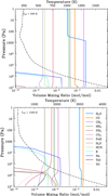 |
Fig. A.1 VMR profiles for all the molecules included in the atmosphere, including non-equilibrium chemistry. These are computed for Teff = 500 K (top panel) and 1500 K (bottom panel), log g = 4 and solar C/O and [M/H] values. H2 and He are not plotted here as they constitute the background and thus the majority of the atmosphere. |
A.2 Line lists and abundances
We provide here the detailed list of abundances and line lists in Table A.1 referred to in Sect. 2.2.1, as well as the element abundances in Table A.2 from Asplund et al. (2021) and an illustration of the error in the previous Exo-REM grid with the proportion of deuterium in the methane isotopologue mixture in Fig. A.2.
Abundances and line lists for selected species.
A.3 Model convergence
Here we present in more detail the process of flagging and eliminating unconverged spectra in the Exo-REM k26 model.
A.3.1 Flags for unconverged grid points
The following are the different types of cases that we considered as unconverged grid points:
Cases which were so unstable that the algorithm crashed, and did not produce an output spectrum or P–T profile. These most likely occur when the input P–T profile is too different from the final solution, and are easily flagged since they manifest simply as a missing grid point.
-
Cases where the output spectrum did not obey the Stefan– Boltzmann law; in a one-dimensional model assuming radiative-convective equilibrium, the net flux F – comprising both radiative and convective components – should be constant across different pressure levels and equal to
 (A.1)
(A.1)We integrated the spectrum over the wavelength range of the model and considered as unconverged those cases for which the total flux deviated by more than 1% from the expected total flux in Eq. A.1.
Finally, some cases may pass criteria 1. and 2. but have an associated P–T profile that contains a large temperature inversion, a drop in temperature with increasing pressure. The thermal structure of a BD and YGP is convective in the deeper layers of its atmosphere, where high electron densities prevent thermal photons from travelling long distances, making convection the primary mode of energy transport (Marley & Robinson 2015). The gradient of a P–T profile in these dense atmosphere zones is taken to follow closely the convective adiabat (Baraffe et al. 2002), and would not contain any temperature inversions. Eventually, as radiation removes more energy from the thinning atmosphere, the temperature gradient with altitude becomes less steep, marking the end of the convective region; here, the thermal profile is governed by radiative equilibrium (Marley & Robinson 2015), tending towards an isotherm at the top layers. There may be small temperature inversions at these layers, but one would not expect to see any dramatic inversions, especially in the deeper, convective layers. Thus, a large temperature inversion beyond the first few layers is a robust marker for an unconverged Exo-REM spectrum, as it is unphysical and only numerically arises from a difficulty for the code to iteratively reach the correct input Teff and total flux. Very high temperatures are required for thermal inversions (> 2500 K), and these occur in the radiative zone (Madhusudhan 2019).
Isotopic abundances (by number) of selected elements. Quantities derived from Asplund et al. (2021).
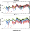 |
Fig. A.2 Methane isotopologue absorption cross-sections at P = 1 bar, T = 500 K, discussed in Sect. 2.2.1. The translucent lines correspond to the R = 106 cross-sections, while the thick and opaque ones are those same cross-sections binned down to R = 500. Top panel: Crosssections for equal abundances of each isotopologue (as was erroneously implemented previously for CH3D in Exo-REM). Bottom panel: Crosssections when weighted according to solar abundances (i.e. D/H ratio of 2 × 10⁻⁵). |
A.3.2 Treatment of unconverged grid points
To minimise the number of missing grid points after a first run of Exo-REM, we have developed a new procedure for the flagged simulations. For those that have crashed (1.), we try again with an adjacent P–T profile which, in practice, is one with the same input parameters and a C/O ratio ± 0.05. We choose to slightly alter this parameter as it is the one that has the least effect on resulting P–T profiles and spectra. Furthermore, we subdivide category 2. into spectra deviating between 1-2% from the total expected flux, and those deviating more than 2%; for the former, we deem that the profiles must not be far from convergence and we rerun Exo-REM with the output P–T profile as a new input, giving it more iterations to converge. For the latter case, we selected, as for category 1., an adjacent P-T profile with C/O ± 0.05 and rerun. Lastly, for category 3. where an inversion is detected in the final T–P profile, we also inject an adjacent P–T profile and start from scratch. In all of these cases, the majority of grid points were able to reach convergence, and those that did not are discarded to avoid biasing the grid with unphysical points. These constituted 0.25% of the cloudless grid, 0.1% of the cloudy microphysics grid and 3.4% of the fsed grid and are listed on the Exo-REM site. The most problematic zones were the high Teff and low fsed values as they were the most unstable.
The most cloudy cases had the largest number of grid points that were not able to converge: this is due to the unstable nature of adding cloud physics to the model. For every iteration of the algorithm, the chemistry is computed with an associated P–T profile; only then are the clouds added, which affects in turn, the thermal structure. However, the chemistry is not recomputed once the clouds are added, and thus if they had a strong impact on the thermal structure, the next iteration will have a drastically different associated profile. As a result, the final spectrum may conserve flux, but it is possible that not each level of the atmosphere is converged, leading to a T–P inversion (category 3.).
A.4 Exo-REM k26 CMD with varying fsed
Fig. A.3 shows the fsed trend along the L–T transition discussed in Sect. 3.2.
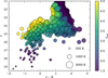 |
Fig. A.3 CMD with the data points sized according to their interpolated Teff, and coloured by their interpolated fsed found by computing the magnitudes of Exo-REM k26 spectra of varying fsed and Teff values at log g = 4.5 and solar C/O and [M/H], then interpolating to find the fsed and Teff at the Best et al. (2025) data points. This highlights the fsed trend discussed in Sect. 3.2 |
Appendix B Posterior distributions
In B.1 we discuss the error bars in the posterior distributions from the forward modelling carried out on VHS 1256 b in Sect. 3.4 and supply all of the posterior distributions for GJ 504 b and VHS 1256 b:
B.1 χ2red and posterior uncertainties in the VHS 1256 b analysis
The Bayesian framework propagates the input data error in the posterior distributions: since the input JWST data for VHS 1256 b has minute error bars (the average across the NIRSpec and MRS data being ~5%), the posteriors are narrow and with a dispersion that does not account for model systematics. The χ2red of the bestfitting models found here, while being considerably smaller than those found in previous studies on the same data, have values much larger than 1, which indicates that errors other than noise dominate the error budget, such as additional flux errors in the JWST data and, more importantly, modelling errors. We carried out an identical run where we multiplied the NIRSpec and MIRI noise error by a factor of 10.6 to bring the value of χ2red for the best-fitting model to 1.0. This is similar to the approach of Gibson et al. (2020), who introduced a β parameter to scale the noise amplitude and modified accordingly the likelihood function, as well as Zhang et al. (2025) who added noise, through an hyperparameter log b, to their NIRSpec data. Our test, as intended, brought the final  to 1 and inflated the ±1σ values of each posterior distribution: each parameter went from an error of ~0.02% to −0.2%, with the exception Teff that increased from −0.06% to −0.9%. Although this had the effect of amplifying the ±1σ values by a factor of −10, these are nonetheless still misrepresentative of the actual error on this analysis that is dominated by model systematics, and we show the original, non-inflated distributions in Figs. 7, 8 and 9. Furthermore, the solutions tend to converge to grid nodes, (e.g. [M/H] = 1.50 dex, and C/O = 0.55 for the MIRI/MRS fit). This is a recurring issue when using precomputed grids, whereby grid points that are synthesised directly by the model will sometimes have appreciably higher likelihoods than the adjacent interpolated spectra.
B.2 Corner plots
In Figs. B.1–B.4, we provide the posterior distributions associated with each forward modelling analysis described in the main text.
Appendix C Longitudinal heterogeneity fraction calculation
In Sect. 4.3 we calculate the fraction of longitudinal heterogeneous cloud cover, using the fluxes from each of the fsed solutions derived in the two-column approach. Here we detail the method. We suppose that, in the two-column framework, the maximum and minimum fluxes produced along a light curve are given by
 (C.1)
(C.1)
 (C.2)
(C.2)
with  .
.
 (C.3)
(C.3)
For the 2018 HST observed amplitude 1.2/4.71.of Aobs = 0.247 =  at 1.27 μm, we have
 (C.4)
(C.4)
The average flux at 1.27 µm is taken to be the two-column best-fit solution that we find in Fig. 9 corresponding to α = 0.62; 〈F〉 = 0.62Fthick + 0.38Fthin = 4.89 × 10⁻¹⁶ Wm−2 μm−1. The fractions of thick cloud coverage producing the minimum and maximum of the HST light curve are
 (C.5)
(C.5)
Similarly, for the Spitzer observed amplitude of Aobs = 0.0576 at 4.5 µm we have
 (C.6)
(C.6)
The average flux is 〈F〉 = 2.00 × 10⁻¹⁶ W m−2 μm−1. Therefore, the fractions of thick cloud coverage producing the minimum and maximum of the Spitzer light curve are
 (C.7)
(C.7)
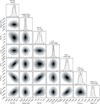 |
Fig. B.1 Posterior distribution from VHS 1256 b forward modelling with ForMoSA using the medium-resolution Exo-REM k26 grid and just MIRI/MRS observations, with only one column (so the classical approach). The 3σ, 2σ, 1.5σ, 1σ, and 0.5σ regions are shown in regions shaded from grey to black (in respective order), and the listed uncertainties correspond to 1σ. The corresponding best fit is shown in Fig. 7. Flat priors are given spanning the whole Exo-REM k26 grid range detailed in Table 1. |
 |
Fig. B.2 Same as Fig. B.1 but using all of the JWST observations. The corresponding best fit is shown in Fig. 8. |
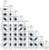 |
Fig. B.3 Same as Fig. B.2 but in a two-column framework as detailed in Sect. 3.4.2. The corresponding best fit is shown in Fig. 9. |
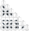 |
Fig. B.4 Posterior distribution from forward modelling with ForMoSA using the GJ 504b photometry with the low-resolution Exo-REM k26 grid. The resulting best-fit model is shown in Fig. 6. |
All Tables
Best-fit parameter values for the GJ 504b photometry using the former version of Exo-REM versus using Exo-REM k26.
Isotopic abundances (by number) of selected elements. Quantities derived from Asplund et al. (2021).
All Figures
|
Fig. 1 Top panel: comparison of the new Exo-REM k26 cloudless grid (coloured) to the previous grid (in grey; Charnay et al. 2018) for models with log g = 4 dex and solar C/O and [M/H]. The difference between the two models at the same Teff is shaded. The most notable differences are due to changes in the Na and K line profiles and the revised CH3D abundance. Bottom panel : relative residual flux (Fnew − Fold)/Fold × 100. |
| In the text | |
|
Fig. 2 Comparison of alkali absorption cross-sections using line lists of Allard et al. (2019) and Burrows & Volobuyev (2003) for Na (left panel) and Allard et al. (2016) and Burrows & Volobuyev (2003) for K (right panel) at P = 10 bar and T = 899.5 K, which are conditions in the atmosphere probed by the ≈ 1 μm peak flux. |
| In the text | |
|
Fig. 3 Spectra from the R = 500 Exo-REM k26 fsed grid coming from almost cloudless cases (fsed = 9) to atmospheres with extremely optically thick clouds (fsed = 0.5). The 1–2 μm flux decreases with fsed, with the thickest cloud cover dampening spectral features the most. In red is a Sonora Diamondback model with fsed = 1, the lowest value explored in their grid; the corresponding Exo-REM k26 model is shown in blue. The other parameters are fixed at Teff = 1200 K, log g = 4.5 dex, and solar C/O and [M/H]. The 8–10 μm inset highlights which fsed values exhibit the silicate absorption. |
| In the text | |
|
Fig. 4 Colour-magnitude diagram with the computed J versus J – K magnitudes for the Exo-REM k26 cloudless log g = 5 (in black) and simple cloud microphysics models (for log g = 3, 3.5, 4, 4.5, and 5 in purple, green, pink, light blue, and blue respectively) at constant solar C/O and [M/H]. The simple microphysics grid was computed with a supersaturation parameter s = 0.1. The M, L, and T dwarfs are plotted in black, red, and blue dots, respectively (Best et al. 2025). Data for GJ 504 b, VHS 1256 b, and HR 2562 b are from Kuzuhara et al. (2013), Gauza et al. (2015), and Konopacky et al. (2016), respectively. |
| In the text | |
|
Fig. 5 Evolution of fsed for BDs over the L–T transition found by computing the magnitudes of Exo-REM k26 spectra of varying fsed and Teff values at log g = 4.5 and solar C/O and [M/H], then interpolating to find the fsed and Teff at the Best et al. (2025) data points. The median over 20 K Teff ranges is shown in black, and the 1σ region is shaded in grey. |
| In the text | |
|
Fig. 6 Best fit for GJ 504 b photometry with revised parameters found with Exo-REM k26, posterior distributions of which are provided in Fig. B.4. Plotted in grey are random samples from the family of spectra with a likelihood within 1 σ of the best fit. Top panel: normalised transmission for each filter. Bottom panel: residual flux between the observed and simulated photometry. |
| In the text | |
|
Fig. 7 Top panel: one-column best fit in black for only the VHS 1256 b MIRI/MRS data (Gauza et al. 2015) from forward modelling with the medium resolution Exo-REM k26 grid. Observation data are coloured according to MIRI channels. Bottom panel: zoom in on the best fit. The 1σ uncertainty is shown in grey in the top panel, and in the bottom panel, it is shown as grey error bars for one out of four points. |
| In the text | |
|
Fig. 8 Top panel: same as Fig. 7 but with the MIRI + NIRSpec VHS 1256 b observations (Gauza et al. 2015). The best fit for the MIRI/MRS spectrum only from Fig. 7 is shown in grey, with reduced resolution for visibility. Bottom panel: residual flux divided by the simulated flux. |
| In the text | |
|
Fig. 9 Final best fit for VHS 1256 b. Top panel : same as Fig. 8 but using the two-column approach. Best-fit parameters are Teff = 1153 K, log g = 4.0 dex, [M/H] = 0.08 dex, C/O = 0.60, and R = 1.2 RJup, with an α = 0.62, so a linear combination of fsed = 0.7 (62%), shown with a grey dashed and fsed = 2.4 (38%) a grey solid line. Both grey fsed components have been scaled by their proportion and multiplied by a factor of 0.6 for visibility. The two fsed component spectra are shown with reduced resolution for visibility. Bottom panel: same as Fig. 8. |
| In the text | |
|
Fig. 10 Zoom in on the final two-column best-fit model (black) and observation (orange) of VHS 1256 b showing, from top to bottom, primarily the CO, alkali, and CH4 absorptions. |
| In the text | |
|
Fig. 11 Vertical cloud structure for both fsed columns used to describe the patchy cloud cover of VHS 1256 b. We show the cumulative forsterite (Mg2SiO4) cloud opacity (from the top layer) at λ = 1 μm and the pressure level corresponding to a cloud opacity of τ = 1 (dashed). |
| In the text | |
|
Fig. 12 Left panel: photospheric pressures, from where most of the thermal emission originates, for both components (atmosphere columns) of the spectrum of VHS 1256 b. The colour indicates the temperature at the respective pressure. Right panel: P–T profile for the fsed = 0.7 (red) and 2.4 (blue) column. |
| In the text | |
|
Fig. 13 Simplified schematic of a possible cloud configuration of VHS 1256 b at the time the JWST observations were recorded. Here we show a physically plausible configuration of waves and spots that could cause the complex sinusoidal rotationally modulated variations reported in Zhou et al. (2022). The fsed = 0.7 region would emanate flux from higher altitude and give rise to silicate absorption, while the fsed = 2.4 region would emanate from lower regions, shaping predominantly the shorter wavelengths of the spectrum. |
| In the text | |
|
Fig. A.1 VMR profiles for all the molecules included in the atmosphere, including non-equilibrium chemistry. These are computed for Teff = 500 K (top panel) and 1500 K (bottom panel), log g = 4 and solar C/O and [M/H] values. H2 and He are not plotted here as they constitute the background and thus the majority of the atmosphere. |
| In the text | |
|
Fig. A.2 Methane isotopologue absorption cross-sections at P = 1 bar, T = 500 K, discussed in Sect. 2.2.1. The translucent lines correspond to the R = 106 cross-sections, while the thick and opaque ones are those same cross-sections binned down to R = 500. Top panel: Crosssections for equal abundances of each isotopologue (as was erroneously implemented previously for CH3D in Exo-REM). Bottom panel: Crosssections when weighted according to solar abundances (i.e. D/H ratio of 2 × 10⁻⁵). |
| In the text | |
|
Fig. A.3 CMD with the data points sized according to their interpolated Teff, and coloured by their interpolated fsed found by computing the magnitudes of Exo-REM k26 spectra of varying fsed and Teff values at log g = 4.5 and solar C/O and [M/H], then interpolating to find the fsed and Teff at the Best et al. (2025) data points. This highlights the fsed trend discussed in Sect. 3.2 |
| In the text | |
|
Fig. B.1 Posterior distribution from VHS 1256 b forward modelling with ForMoSA using the medium-resolution Exo-REM k26 grid and just MIRI/MRS observations, with only one column (so the classical approach). The 3σ, 2σ, 1.5σ, 1σ, and 0.5σ regions are shown in regions shaded from grey to black (in respective order), and the listed uncertainties correspond to 1σ. The corresponding best fit is shown in Fig. 7. Flat priors are given spanning the whole Exo-REM k26 grid range detailed in Table 1. |
| In the text | |
|
Fig. B.2 Same as Fig. B.1 but using all of the JWST observations. The corresponding best fit is shown in Fig. 8. |
| In the text | |
|
Fig. B.3 Same as Fig. B.2 but in a two-column framework as detailed in Sect. 3.4.2. The corresponding best fit is shown in Fig. 9. |
| In the text | |
|
Fig. B.4 Posterior distribution from forward modelling with ForMoSA using the GJ 504b photometry with the low-resolution Exo-REM k26 grid. The resulting best-fit model is shown in Fig. 6. |
| In the text | |
Current usage metrics show cumulative count of Article Views (full-text article views including HTML views, PDF and ePub downloads, according to the available data) and Abstracts Views on Vision4Press platform.
Data correspond to usage on the plateform after 2015. The current usage metrics is available 48-96 hours after online publication and is updated daily on week days.
Initial download of the metrics may take a while.