


| Issue |
A&A
Volume 711, July 2026
|
|
|---|---|---|
| Article Number | A258 | |
| Number of page(s) | 18 | |
| Section | Interstellar and circumstellar matter | |
| DOI | https://doi.org/10.1051/0004-6361/202558772 | |
| Published online | 21 July 2026 | |
JOYS+: A JWST/MIRI survey of the evolution of H2 winds and jets from low-mass protostars
1
Leiden Observatory, Leiden University,
PO Box 9513,
2300 RA
Leiden,
The Netherlands
2
Max-Planck-Institut für Extraterrestrische Physik,
Giessenbach-strasse 1,
85748
Garching,
Germany
3
INAF – Osservatorio Astronomico di Capodimonte,
Salita Moiariello 16,
80131
Napoli,
Italy
4
Institut de Ciències de l’Espai (ICE-CSIC),
Campus UAB, Can Magrans S/N,
08193
Cerdanyola del Vallès,
Catalonia,
Spain
5
Institut d’Estudis Espacials de Catalunya (IEEC),
c/Gran Capita 2–4,
08034
Barcelona,
Catalonia,
Spain
6
Max Planck Institute for Astronomy,
Königstuhl 17,
69117
Heidelberg,
Germany
7
Department of Physics,
PO Box 64,
00014
University of Helsinki,
Finland
8
Jet Propulsion Laboratory, California Institute of Technology,
Pasadena,
CA
91109,
USA
9
European Southern Observatory,
Karl-Schwarzschild-Strasse 2,
85748
Garching bei München,
Germany
10
Université Paris-Saclay, CNRS, Institut d’Astrophysique Spatiale,
91405
Orsay,
France
11
Department of Astronomy, University of Virginia,
Charlottesville,
VA
22903,
USA
12
Virginia Institute of Theoretical Astronomy, University of Virginia,
Charlottesville,
VA
22903,
USA
13
School of Cosmic Physics, Dublin Institute for Advanced Studies,
31 Fitzwilliam Place,
Dublin 2,
Ireland
14
National Radio Astronomy Observatory,
520 Edgemont Rd.,
Charlottesville,
VA
22903,
USA
15
INAF – Osservatorio Astronomico di Roma,
Via di Frascati 33,
00078
Monte Porzio Catone,
Italy
16
Joint ALMA Observatory,
Alonso de Córdova 3107,
Vitacura,
Santiago,
Chile
17
Institut de Ciències de l’Espai (ICE, CSIC),
Can Magrans s/n,
08193
Cerdanyola del Vallès,
Catalonia,
Spain
18
Institut d’Estudis Espacials de de Catalunya (IEEC),
08034
Barcelona,
Catalonia,
Spain
19
Department of Astrophysics, University of Vienna,
Türkenschanzs-trasse 17,
1180
Vienna,
Austria
20
ETH Zürich, Institute for Particle Physics and Astrophysics,
Wolfgang-Pauli-Strasse 27,
8093
Zürich,
Switzerland
21
Department of Astronomy, Oskar Klein Centre, Stockholm University, AlbaNova University Center,
10691
Stockholm,
Sweden
22
UK Astronomy Technology Centre, Royal Observatory Edinburgh,
Blackford Hill,
Edinburgh
EH9 3HJ,
UK
23
School of Cosmic Physics, Dublin Institute for Advanced Studies,
31 Fitzwilliam Place,
Dublin 2,
Ireland
★ Corresponding author: This email address is being protected from spambots. You need JavaScript enabled to view it.
Received:
23
December
2025
Accepted:
13
April
2026
Abstract
Context. The base of protostellar outflows can display both wide-angle, low-velocity winds and high-velocity, collimated jets, the magnetocentrifugal launching of which enables accretion onto the protostar. In outflows from the youngest protostars, the majority of the ejected or entrained mass is likely molecular H2 . How the H2 outflow evolves as the central protostar grows and the envelope dissipates is important for understanding the nature of the launching mechanism and assembly of the nascent protostar.
Aims. Using JWST MIRI/MRS observations with an unprecedented spatial resolution down to 0.3" towards 13 single and 20 multiple Class 0 and I protostars, we aim to investigate the H2 wind and jet morphology, mass outflow rate, velocity and temperature structure, and the evolution of these properties with protostellar class.
Methods. We constructed continuum-subtracted maps of the H2 S(1) and S(7) line flux and velocity towards the outflows in our sample and ALMA sub-millimetre CO maps. Towards the base of each blueshifted outflow lobe (typically within 300 au), we extracted representative spectra and measured the outflow opening angles from the H2 S(1) line emission. A rotation-diagram fitting of the H2 lines was used to determine the column density and temperature, which was combined with measurements of the outflow width and H2 line velocity to measure the mass-loss rates.
Results. Low- J (J ≤ 4) transitions of H2 largely trace extended wide-angle, low-velocity (0-20 km s−1) winds within the contours of the low-velocity (<30 km s−1) sub-millimetre CO emission, while high-J (J > 5) transitions are associated with shocks and knots. In Class 0 sources with a known high-velocity (>30 km s−1) molecular CO or SiO jet, higher H2 velocities are observed along the jet axis. The opening angle of the wind traced by the H2 S(1) line broadens from ∼20° to ∼90° through the Class 0 to the Class I stage. The rotation diagrams in the blueshifted outflow lobes show a clear separation between a warm, ∼600 K and a hot, 1500-3000 K component, with no clear sign of evolution in the excitation temperature. The warm component contains two orders of magnitude more mass than the hot component, and the H2 outflow mass-loss rate declines by two orders of magnitude from the Class 0 to the Class II stage. A correlation with the bolometric luminosity of the driving source is observed. A factor of 10–1000 mismatch between the warm H2 and cold sub-millimetre CO outflow rate and momentum flux is also seen, which is consistent with the presence of cold and likely entrained (<150 K) molecular H2 that cannot be detected with JWST/MIRI.
Conclusions. The declining warm H2 mass-loss rates and increasing opening angles from the Class 0 to I stages – and the absence of H2 jets in the Class I sources – are consistent with the predictions of magnetohydrodynamical (MHD) disc wind models; however, the relatively constant temperatures of the warm and hot components with evolutionary stage may reflect the typical conditions in the outflow shocks rather than temperature stratification of the wind.
Key words: stars: formation / ISM: jets and outflows
© The Authors 2026
 Open Access article, published by EDP Sciences, under the terms of the Creative Commons Attribution License (https://creativecommons.org/licenses/by/4.0), which permits unrestricted use, distribution, and reproduction in any medium, provided the original work is properly cited.
This article is published in open access under the Subscribe to Open model. This email address is being protected from spambots. You need JavaScript enabled to view it. to support open access publication.
1 Introduction
Low-mass young protostars are nearly universally found to be associated with bipolar outflows of gas. These flows have a variety of components that are mainly distinguished by their velocity and degree of collimation angle (Bachiller 1996; Ray et al. 2007; Bally 2016). Towards Class I protostars, collimated and high-velocity (≥30 km s−1) jets are frequently detected in atomic lines, but they also show a molecular component in rovibrational H2 lines (Davis et al. 2001, 2011; Frank et al. 2014). The younger Class 0 protostars additionally show high-velocity jets traced by CO, SiO, and SO millimetre lines (Lee 2020; Podio et al. 2021) and far-infrared (far-IR) H2O lines (Kristensen et al. 2012). In addition to the jet, low-velocity and wide-angle ‘winds’ are frequently observed towards young protostars (Zapata et al. 2015; Bjerkeli et al. 2016; Lee et al. 2018; Tabone et al. 2017; de Valon et al. 2020). On large scales (≥0.1 pc), an entrained and cold ‘outflow’ component traced by low-J CO lines is observed (Frank et al. 2014; Bally 2016). The term outflow is also used in a more general sense to refer to any gas moving away from the protostar, including the winds and jets (see van Dishoeck et al. (2025) for terminology).
The wide-angle winds and collimated jets are both thought to be magnetocentrifugally launched and to mediate accretion by extracting angular momentum from the disc, allowing disc material to move inward towards the protostar. The exact launching mechanism and location for the winds and jets is debated (Pascucci et al. 2023). While both X-winds, which are launched from the interaction point between the stellar magnetosphere and inner disc (e.g. Shu et al. 1994; Shang 2007; Shang et al. 2023), and MHD disc winds, which are launched over an extended region of ∼1-100 au (e.g. Blandford & Payne 1982; Pudritz & Norman 1983; Casse & Keppens 2002; Zanni et al. 2007), are consistent with observations to a varying degree, the detection of rotating molecular winds with footpoints in the outer discs of protostars (e.g. Lee et al. 2018; Tabone et al. 2017; Nazari et al. 2024) provides strong evidence in favour of the disc-wind scenario. Thermal photo-evaporative winds from more evolved Class II discs may play an important role in eventually dispersing the disc, but they are not likely to be effective in the younger Class 0 and I sources (Ercolano & Pascucci 2017).
Regardless of the underlying launching mechanism, observing wind and jet evolution in the earliest stages of star formation is important for understanding the assembly of the protostar and setting of the initial disc conditions for planet formation. A variety of broad trends are known: the mass-loss rate of outflows as traced by sub-millimetre CO (Bontemps et al. 1996; Mottram et al. 2017) or mid-IR and far-IR line–luminosity relations (Watson et al. 2016; Karska et al. 2018) is strongly correlated with the bolometric luminosity of the protostar and anti-correlated with the evolutionary stage. The structure of the outflows evolves as well, as the composition shifts from largely molecular (Class 0 and I protostars) to atomic (Class II discs) (Nisini et al. 2015; Lee 2020), and the sub-millimeter CO component increases in opening angle from the Class 0 to I stage (Dunham et al. 2024).
While winds and jets from evolved Class II sources are readily observable in a wide variety of tracers, in the younger Class 0 and I protostars, much heavier extinction by the nascent envelope makes it difficult to observe the winds and jets at their launching point at wavelengths shorter than the sub-millimetre. With the launch of the James Webb Space Telescope (JWST), it is now possible to probe the winds and jets from young embedded sources at unprecedented sensitivity in a variety of near- and mid-IR lines. Of particular interest are the rotational and rovi-brational lines of H2, which uniquely occur at near- and mid-IR wavelengths and directly probe the dynamics of the dominant molecular component of the outflows. Thermochemical modelling of magnetocentrifugally launched winds suggests that H2 offers an excellent tracer of the bulk mass and momentum-loss rates (Tabone et al. 2020; Rab et al. 2022). The NIRSpec and MIRI/MRS instruments on the JWST provide coverage of the rovibrational and pure rotational lines of H2, respectively. The low-J S(1) to S(8) rotational lines observable with MIRI/MRS are especially useful, as they provide reliable measurements of the H2 column density and ortho-to-para ratio over gas temperatures of ∼100-3000 K (Neufeld et al. 1998; Rosenthal et al. 2000).
Historically, ground-based observations of the H2 v = 1-0 S(1) 2.12 µm line have been used to study Herbig–Haro objects: bright nebular emission from shocks where the outflow interacts with the ambient ISM at distances far from the protostar (Reipurth & Bally 2001). At the outflow launching point, a slow and wide-angle H2 wind component from Class I protostars was first identified through 2.12 µm emission by Davis et al. (2001), and subsequently its extent in spatially observations spectra was shown to be of a few hundred astronomical units (Davis et al. 2011; Garcia Lopez et al. 2013). Infrared Space Observatory (ISO) observations of protostellar outflows first identified emission from low- J rotational H2 lines with temperatures from ∼600-3000 K, sometimes with an ortho-to-para ratio (OPR) < 3 (Neufeld et al. 1998; Nisini et al. 1999; Rosenthal et al. 2000). With the launch of Spitzer, mid-IR observations of the rotational H2 lines subsequently identified warm (300–600 K) and hot (∼1000 K) H2 emission in more outflows (e.g. L1448-mm (Dionatos et al. 2009) and HH 211 Dionatos et al. 2010). Far-IR observations with Herschel of the warm outflowing gas in high-J CO transitions also found a similar distribution of temperature components (Manoj et al. 2013; Karska et al. 2018).
With the increased sensitivity and spatial resolution of the JWST, studies on the H2 wind and jets near their launching region in the disc have begun. NIRSpec observations of outflows from edge-on Class I and II discs have commonly identified collimated high-velocity jets traced in [Fe II] lines surrounded by conical emission traced by the H2 S(9) and v = 1-0 S(1) lines (Delabrosse et al. 2024; Pascucci et al. 2025; Harsono et al. 2023); a similar morphology is found in MIRI/MRS and NIRSpec observations of outflows from younger and more embedded protostars (Narang et al. 2024; Federman et al. 2024; van Dishoeck et al. 2025). Caratti o Garatti et al. (2024) identified a wide-angle wind component in warm H2 from the base of the very young Class 0 protostar HH 211 and found that the majority of the mass loss was carried by the molecular component of the outflow. In some nearby protostars, MIRI/MRS observations of the pure rotational lines have revealed a trend of the opening angle increasing with decreasing excitation energy (e.g. TMC1, Tychoniec et al. 2024, HOPS 315, Vleugels et al. 2025), though this does not appear to be the case in other objects (e.g. Ced110 IRS4, Narang et al. 2025).
In this work, we aim to expand on recent JWST studies of H2 winds and jets by using the substantial JOYS+ sample of Class 0 and I protostars observed with JWST/MIRI (Wright et al. 2023) to measure the H2 mass-loss rates, momentum-flux rates, and morphology across the largest sample to date. More detailed analyses of a few individual JOYS sources with 3 × 3 or larger mosaics are also presented in Caratti o Garatti et al. (2024, HH 211), Tychoniec et al. (2026, BHR71 IRS1), and Navarro et al. (in prep., L1448-mm).
The remainder of this paper is organized as follows. In Section 2, we describe our sample, the JWST data, and accompanying archival ALMA data. In Section 3, we present line flux and velocity maps of our sources in H2 and sub-millimetre CO and describe our analysis of the outflow opening angles, mass-loss rates, and momentum fluxes. We present trends in evolutionary stage and bolometric luminosity and discuss the interpretation of the outflow morphology and evolution in terms of MHD disc winds in Section 4. We provide a summary of our results and conclusions in Section 5.
2 Observations
The data comprising our sample consists of 25 MIRI/MRS observations selected from programmes 1290 (JOYS, van Dishoeck et al. 2025), 1236 (Perseus Binaries, Ressler et al., in prep.), and 1257 (HH 211, Caratti o Garatti et al. 2024), the details of which are summarized in Table 1. All low-mass sources from these programmes are included, with the exceptions of B1-b and B1-bS, which are too heavily extincted for useful measurements of the H2 emission; ASR-106, a Class I binary with faint H2 emission and no clear outflow activity; and SVS 4–5, a background source included in JOYS for studies of ice absorption.
The data for programmes 1236 and 1290 were reduced using the JWST pipeline 1.16.1 (Bushouse et al. 2025) with the CRDS context file jwst_1293.pmap following the procedures described in van Gelder et al. (2024). For data reduction on the 1257 programmes, see (Caratti o Garatti et al. 2024). The reduction followed standard pipeline, including a fringe flat correction for the extended sources (Crouzet et al. 2025), followed by the residual fringe correction step and a dedicated sky background applied at the detector level in the Spec2 step of the pipeline. An additional 1D residual fringe correction (Kavanagh, in prep.) was applied to the extracted spectra described in Section 3.3. The default step of outlier rejection was turned off, and instead a custom-made bad-pixel routine was applied using the VIP package (Christiaens et al. 2023).
The MIRI/MRS integral field unit provides a spectral resolving power of R = ∆λ/λ = 3500-1500, and a spatial resolution from 0.3-1.0″, both decreasing across the wavelength range (Law et al. 2023). For the shortest wavelength H2 lines, this corresponds to spatial scales as small as 41 au for targets in Taurus and up to 125 au for the most distant targets in Serpens, and we were thus able to reach scales comparable to the disc diameter in these cases. The field of view of a single MIRI/MRS pointing increases with wavelength from 3.2 × 3.7″ to 6.6 × 7.7″. The majority of our observations are single pointings of MIRI/MRS, and those from programme 1290 are typically centred on the blueshifted outflow lobe; those from 1236 are centred towards the binary protostar positions. Several observations from programme 1290 are mosaics with two to four pointings: IRAS4B, B1-c, Ser-SMM1, L1448-mm, BHR71-IRS1, BHR71-IRS2 (see Table A.1 of van Dishoeck et al. 2025). The blueshifted lobe of HH 211 is covered by the extensive mosaic described in Caratti o Garatti et al. (2024).
To map the spectrally integrated flux in the H2 lines, we jointly fitted a Gaussian and a linear-continuum model to each spaxel in the MIRI/MRS cubes. This is analogous to a continuum subtracted moment 0 map, but we find this method better recovers emission in regions with both low signal-to-noise (S/N) and low line-to-continuum ratios. Fitting a Gaussian also allows the velocity centroid of the H2 lines to be measured, providing a result similar to that of a moment 1 map. Although spectral lines of H2 are generally unresolved by MIRI/MRS, it is still possible to measure velocity shifts of the H2 lines via centroiding at less than the nominal spectral resolution, with a precision of ∼c/(R √S/N), where c is the speed of light.
To complement the JWST data, we collected archival ALMA observations of the CO 2–1 and 3–2 lines to trace the entrained gas component of the outflow. The programmes used, details of the observations, and the data-reduction reference per source are listed in Table B.1. For each source, we created moment 0 and moment 1 maps of the CO emission integrated from the source velocity to ±2-30 km s−1. The CO emission within 2 km s−1 was excluded as it is contaminated by large-scale emission in the cloud.
We aim to use our observations to examine evolutionary trends across the sample. As proxies for the source evolution, we used the bolometric temperature Tbol and luminosity Lbol (Myers & Ladd 1993), as well as the envelope mass Menv where available. The bolometric temperature increases monotonically with source age, with a boundary defined between the Class 0 and I protostars at 70 K, and between Class I protostars and the Class II protoplanetary discs at 650 K (Chen et al. 1995). We note that the bolometric luminosity is the sum of contributions from the stellar photosphere and reprocessed accretion, and it was previously thought to be dominated by the accretion component for Class 0 protostars. Models of magnetocentrifugally driven outflows predict that wind mass-loss rates should scale with the accretion rate, a trend that is consistent with the observed correlation between protostellar mass-loss rate and bolometric luminosity as a proxy for accretion (Watson et al. 2016). However, a recent attempt to separate the contributions of the stellar photosphere and accretion luminosity in protostars with well-constrained dynamical masses found the bolometric luminosity for most objects was consistent with emission largely from the photosphere (Hartmann et al. 2025).
We caution that Lbol, Tbol, and Menv were determined from lower resolution observations that do not spatially resolve multiple sources. In Table 1 we state whether a source is single or multiple on scales <3″ as determined from interferometric observations. Where needed, we re-scaled the source luminosity using the most up-to-date distances to the cloud or individual sources available.
MIRI/MRS observation sample.
3 Analysis and results
In this section, we present maps of the H2 intensity and velocity and describe our analysis of the H2 rotational lines. We focus on the v = 0-0 pure rotational ΔJ = +2 lines, the S(1) to S(8) of which are typically detected. We first constructed line flux and velocity centroid maps, and also fit the opening angle of the wide-angle H2 emission as traced by the S(1) line. We compare the H2 emission with ALMA maps of the blueshifted and red-shifted CO to examine the outflow morphology evolution. We extracted spectra of the H2 emission in apertures placed in the blueshifted lobe of each source. A rotation diagram analysis was used to determine the H2 column density and excitation temperature in each aperture and to estimate the extinction. Outflow rates are computed by combining measurements of the H2 velocity with the column densities from the rotation diagram and outflow extent.
3.1 H2 line maps
We present line flux maps of the ALMA CO (first row), H2 S(1) (second row), and H2 S(7) (third row) in Figures 1 to 2. The panels are ordered in increasing bolometric temperature as a proxy for the evolutionary stage. The central protostar position(s) traced by the millimetre continuum are marked by a white star. These positions are taken from the literature (Tobin et al. 2016; van’t Hoff et al. 2020; Yang et al. 2020; Gavino et al. 2024; Hull et al. 2017; Lee et al. 2018) or fitted to publicly available ALMA millimetre continuum images (Programme 2017.1.01350.S). The moment 1 map of the ALMA CO and the centroid velocity maps for the same H2 transitions are shown in the same manner in Figures 3 and 4.
Figures 1-4 shows a clear difference in morphology of the H2 S(1) and H2 S(7) lines; the extended S(1) (Eup/k ~ 1000 K) line mostly traces a slow (∼10 km s−1) and wide-angle wind component, while the S(7) (Eup/k ∼ 7200 K) emission is compact and associated with shock knots and/or a collimated jet. However, we note that the S(1) line also becomes brighter towards the shock positions, likely reflecting higher column densities from compression in the shocks and/or higher temperatures. We note that there is typically faint emission from low-J H2 that is not clearly associated with the outflow detected throughout the map, possibly arising from ambient cloud material along the line of sight.
The overall extent of the H2 S(1) emission is quite similar to the lower velocity (0–30 km s−1) CO in the blueshifted lobes, though it is much brighter within the outflow cavity. In contrast to the CO, the H2 emission is typically much fainter or entirely undetected in the redshifted lobe, where the extinction is higher as a result of the outflow cavity inclination and, thus, the higher column density of intervening dense envelope material.
Inspection of the maps reveals clear trends with evolutionary stage as traced by the bolometric temperature. The H2 emission is much fainter towards the more evolved Class I sources, where it is typically brightest at the protostellar position traced by the millimetre continuum. This is in contrast to the Class 0 sources, where there is much greater extinction from the envelope at the outflow base. The majority of the Class 0 sources in our sample are known to have high-velocity molecular jets traced by sub-millimetre CO, SiO, or SO (see Table 1). In all targets with molecular jets, radial-velocity stratification is seen in the S(1) line velocity maps, and there is a collimated jet with projected velocities of ∼25 km s−1 (Figure 3). None of the Class I sources in the sample show evidence of a collimated jet component in the high-J H2 lines; however, atomic jets towards Class I discs are common and have been detected in most sources in our sample (Tychoniec et al. 2024; van Dishoeck et al. 2025, Ressler, in prep.) and in other JWST protostar studies (Pascucci et al. 2025).
Many of our sources are close binaries or multiple systems with a separation of <500 au (e.g. IRAS 2A, TMC1). In most cases, one member of the binary dominates the driving of a wide-angle H2 wind as traced by the H2 S(1) line. This is seen in both the Class 0 stage (e.g. L1448 IRS 2) and Class I stage (e.g. TMC1, Tychoniec et al. 2024). Differences in the outflow properties between binary members could reflect differences in source evolutionary stage, mass, or a quiescent versus active accretion state. However, we caution that in the deeply embedded sources the absence of visible H2 emission can also be caused by differing levels of extinction towards different members of the binary. This seems to be the case for NGC 1333 IRAS 4A, where submillimetre CO outflows are clearly driven by both sources, yet only the blueshifted lobe of the eastern source is clearly detected in H2 . Further discussion of differences between the close binaries in our sample is presented in van Dishoeck et al. (2025) and Ressler (in prep.).
3.2 Outflow opening angles
The opening angles of protostellar outflows traced by submillimetre CO are known to broaden with increasing bolometric temperature in the Class 0 stage, reaching a maximum of ∼90 degrees in Class I sources, which do not show any further evolution (Arce & Sargent 2006; Dunham et al. 2024). This has been interpreted as the carving out of an increasing solid angle of the outflow cavity with time by a wind (Offner et al. 2011). Given the similarity between the H2 S(1) and sub-millimetre CO emission, we aim to quantify if a similar opening angle trend also exists here. For sources with a clear conical outflow morphology, the outflow opening angle can be measured using the extent of the faint emission from the H2 S(1) line in the blueshifted lobe. The redshifted lobe is typically too extincted or not sufficiently covered by the observations for an opening-angle measurement.
To measure the opening angle, we first rotated the line-flux map so the blueshifted lobe points to the bottom of the image, and we re-sampled the image using cubic spline interpolation (upper panel of Figure 5). We then found candidate edge points using a method similar to that of Narang et al. (2024); that is, we calculated a second-order finite difference in horizontal slices averaged over a vertical width of 3 spaxels and identified local maxima in regions with sufficiently high S/N (lower panel of Figure 5). A selection of edge points near the outflow base was made by visual inspection, and the full opening angle was measured between two linear fits to either side of the cavity. We note that the measured opening angles are somewhat affected by inclination (see Dunham et al. 2024); however, we did not apply an inclination correction. We also note that the absolute value of the opening angle measured is dependent on the wind structure. Temperature, density, and chemical stratification in the wind can affect the apparent opening angle traced by emission lines with different excitation energies (e.g. TMC1, Tychoniec et al. 2024). Our opening angle measurement uses the lowest excitation H2 line available, which should come closest to approximating the widest opening angle of the outflow. The opening angles for the entire sample are provided in Table D.1.
We examine the change in opening angle with increasing bolometric temperature in the upper panel of Figure 6. The opening angle clearly broadens from the Class 0 to the Class I stage, though there is a significant degree of scatter (∼60°) between the Class I sources. A quite similar result was previously found for the cold CO component in a survey of Perseus outflows by Dunham et al. (2024). As the extent of the faintest H2 S(1) emission used to measure the opening angle corresponds well with the same emission in the cold CO, this indeed suggests they may be tracing a similar component in the outflow (Figures 1 and 2). The opening angle is also weakly anti-correlated with the envelope mass of the driving source, as shown in the lower panel of Figure 6. This is expected, as the envelope mass should decline with source evolutionary stage. We discuss further in Section 4.3 whether the opening angle evolution reflects dissipation of the envelope via entrainment or evolution of the wind.
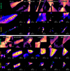 |
Fig. 1 Continuum-subtracted line maps of our sample ordered by bolometric temperature. First and fourth rows: CO 3–2 or 2–1 emission integrated from ±30 km s−1 of the source velocity. Second and fifth rows: integrated H2 S(1) line emission. Third and sixth rows: Integrated H2 S(7) emission. The location of the sub-millimetre peak tracing the protostar driving the outflow is marked by a white star, while the centre of the aperture used for measuring the outflow properties is marked by a red cross. The position of additional apertures used in select sources for comparison of outflow properties with distance are marked by a green plus. The diameter of the apertures is indicated by the scale bar in the lower right. The JWST MIRI/MRS PSF or ALMA beam size is indicated in the lower left. All maps are shown with a logarithmic scaling from three times the RMS noise to the maximum intensity of the map. |
 |
Fig. 3 Continuum-subtracted line centroid and moment 1 maps of our sample ordered by bolometric temperature, annotated as described in Figure 1. First and third rows: moment 1 map of CO 3–2 or 2–1 emission integrated from ±30 km s−1 of the source velocity. Second and fourth rows: velocity centroid of H2 S(1) line from Gaussian fit per pixel. All maps are integrated from −30 to +30 km s−1 . For the ALMA CO maps, the low-velocity cloud at emission at vLSR ± 2 km s−1 is excluded. All maps are masked by using the corresponding moment 0 to apply a black mask with increasing transparency in brighter areas. |
3.3 Outflow spectra extraction
We aim to compare properties of the outflows across both our entire sample and within individual outflows. We therefore extracted at least one spectrum from an aperture in the blueshifted lobe for each source and multiple spectra in apertures following the centre of the outflow axis for a representative subset of four Class 0 (HH 211, L1448-mm, BHR71 IRS1/IRS2) and three Class I sources (TMC1, TMC1A, B1-a). This subset of the observations was selected based on field of view and to sample a range of Class 0 and I sources. For the remaining sources, we extracted a single aperture as close to the protostar position as possible. Near the base of the outflow, the contribution from the wind-angle wind should be greatest, as at positions at greater distances the H2 emission may be dominated by entrained gas. The positions of the extracted apertures used for comparison of the outflows across the sample are shown as red plus symbols in Figures 1-4, while those used for comparison within a single source are shown as green crosses. A 300 au radius aperture with a fix size with wavelength was used for all sources except for TMC1 and TMC1A in Taurus, where their distance of 149 pc allowed a smaller 100 au aperture to be used. The aperture sizes were chosen to adequately sample the MIRI/MRS PSF at the wavelength of the H2 S(1) line.
3.4 H2 line-fitting and rotation diagrams
For each aperture, we extracted line fluxes from the v = 0–0 S(1) to S(8) lines using a fit of a Gaussian and linear baseline in the same manner as the velocity maps (Section 3.1). All eight v = 0– 0 transitions in the MIRI/MRS range were generally detected. We note that the S(0) line of H2 at 28.21883 µm is within the nominal range of MIRI/MRS, but the calibration quality and instrumental sensitivity was generally not sufficient to detect it. In a handful of bright shock positions (e.g. NGC 1333 IRAS 4B), v = 1–1 pure rotational lines were also detected; however, we did not fit them as they provide only slightly more information on the bulk H2 gas properties, though they may be useful for detailed determination of shock properties (Kristensen et al. 2023).
As the critical densities of the v = 0–0 H2 transitions are low enough for LTE to hold even in the low density of a pro-tostellar outflow (Le Bourlot et al. 1999), the temperature and column density of the H2 can be reliably derived through a rotation diagram analysis. For each outflow aperture, we thus fitted a two-temperature component model to the rotation diagram of the pure rotational lines following Francis et al. (2025). This model also simultaneously fits for the extinction and ortho-to-para ratio of the H2. The differential extinction of the S(3) line in the 10 µm silicate feature relative to other nearby H2 lines gave an estimate of the total overall extinction, provided an assumed extinction law was available. We used the KP5 extinction curve of Pontoppidan et al. (2024), which has been shown to provide a reasonable correction for the H2 lines (e.g. Francis et al. 2025). However, we note that the choice of extinction curve remains uncertain, and extinction in the mid-IR likely varies between different clouds and environments (Navarro et al. 2025). We thus report the optical depth of the extinction curve at the S(3) line τS(3) to facilitate comparison with other curves.
An example rotation diagram fit is presented for the Ser-SMM3 outflow in Figure C.1, while the best-fit parameters for all rotation diagram fits are summarized in Table C.1. The H2 emission towards our sources is well described by a warm ∼500–700 and a hot ∼2000–3000 K component, where the warm component’s column density is typically two orders of magnitude higher than that of the hot component. A colder component of H2 could be present, as seen in ISO and Spitzer observations of the S(0) line (e.g. van Dishoeck et al. 1998; Nisini et al. 2010). However, we note our observations are typically sensitive enough to detect H2 in the Class 0 sources at temperatures as low as 120 K. In general, the warm H2 column density and temperature are well constrained, to ∼0.25 dex and ∼85 K, respectively.
 |
Fig. 4 As Figure 3 but for the remainder of our sample. For the Class I sources with a very bright mid-IR continuum (last row), the H2 S(7) velocity centroid is masked out in bright regions close to the protostar where a line centroid cannot be reliably measured. |
 |
Fig. 5 Example of outflow angle measurement from the H2 S(1) line for the case of BHR-71 IRS 2 (see text). |
 |
Fig. 6 Measured opening angle in H2 S(1) emission for our sample versus bolometric temperature (top panel) and envelope mass (bottom panel). Symbols for Class 0 sources are filled diamonds, while Class I sources are shown as open diamonds. |
3.5 H2 mass-loss rates
For each blueshifted outflow lobe, we infer the H2 mass loss rate following the method of Delabrosse et al. (2024) used for the DG Tau B disc wind:
 (1)
(1)
where NH2 is the average H2 column density in an aperture within a given position in the outflow derived from the rotation diagram analysis, Lperp is the transverse width of the H2 emission across the outflow measured from the continuum-subtracted line flux map, and vperp is the velocity of the H2 emission after correcting for inclination.
We calculated the outflow rate for the warm component in all cases and for the hot component where there are sufficient high-J lines detected. We derived the width, Lperp, of the outflow using the S(1) line and assumed the hot component to have the same width as the warm component. We note that the hot component is mostly associated with bright shock knots and appears narrower than the S(1) line in general, so this is formally an upper limit on Lperp. A lower limit can be obtained from constraints on the jet width from resolved atomic lines such as the 5.34 µm line of [Fe II], though we defer this to future papers focusing on the jet (see Caratti o Garatti et al. 2024; Tychoniec et al. 2024). We measured the velocity of each component from the average velocity of the S(1) to S(4) lines for the warm component, and the S(5) to S(8) lines for the hot component. The velocity was corrected for inclination of the outflow, which was estimated from the resolved millimetre disc where available and otherwise estimated visually from the CO cubes following Yıldız et al. (2015). For Per-emb 8 and all Class I sources, the hot H2 velocity is not well determined due to the low S/N or complexity of the emission, and a vperp of 10 km s−1 was instead assumed. Uncertainties on the reported mass-loss rates incorporate the statistical uncertainty on the H2 column density and velocity and the outflow inclination.
As discussed in Section 3.3, a comparison of the H2 emission properties from the rotation diagram fitting and the derived mass-loss rates can be performed both between sources in the sample and within a single outflow. The latter comparison is important for understanding how sensitive the outflow rate measurements are to the location of the extracted spectra. To explore the effect of radial variations, in Figure 7 we show a comparison of the warm H2 properties and the outflow mass-loss rates as a function of distance from the protostar for four Class 0 and three Class I sources. An analogous figure for the hot component is provided in Appendix A. The top panel of Figure 7 compares the total mass in each aperture assuming the H2 emission is optically thin and fills the entire aperture with a constant column density. The H2 mass was scaled to a 100 au radius aperture size to match the smallest apertures chosen for TMC1 and TMC1A. In the inner hundreds of astronomical units up to ∼1000 au, the H2 mass drops by a factor of a few. In HH 211, the H2 mass can only be measured from ∼1500 au when the extinction is sufficiently diminished, and an increase of a factor of a few is seen after this point. The warm H2 excitation temperature (second panel) varies from ∼600–800 K, with higher temperatures in positions extracted from shock knots (see Figures 1-2). For all sources, the outflow widens in a power-law fashion with distance from the protostar (third panel), while the inclination-corrected H2 velocity increases (fourth panel). The combination of the decreasing H2 mass with the increasing outflow width and H2 velocity results in a remarkably constant change in H2 mass-loss rate with distance (bottom panel), which is consistent with conservation of mass within the outflow. The same behaviour is seen for the hot component’s mass-loss rate in Appendix A.
Transverse gradients in velocity and column density may also affect the measured outflow rates. In Section 3.1, we note that the majority of Class 0 sources with known molecular jets have a higher H2 velocity in the outflow centre (by up to a factor of a few) compared with the edges. A similar gradient is typically seen in the H2 column density, and our H2 outflow rate estimates may thus be overestimated by in the younger sources. This will be addressed in more detail in a study of L1448-mm (Navarro et al., in prep.). Overall, we conclude that the choice of aperture position contributes relatively little to the uncertainty in the mass-loss rate (at most a factor of a few), with some bias towards higher estimates in Class 0 sources with strong molecular jets.
 |
Fig. 7 Variation of warm H2 outflow properties with deprojected distance from the protostar. The outflow width (third panel) is determined from the H2 S(1) line map (Figures 1–2). The velocity error bars do not include the systematic error associated with inclination correction. |
 |
Fig. 8 Best-fit excitation temperature of the warm (red circles) and hot (blue triangles) components versus bolometric temperature towards each aperture used for outflow mass-loss measurement in our sample. The shaded regions indicate the average uncertainty on each quantity. The Tbol = 70 K boundary between Class 0 and I sources is indicated by the dashed line, and Class I sources are plotted as open symbols. |
4 Discussion
4.1 Outflow property evolution: H2 temperature, mass, and velocity
To examine trends in the H2 emission properties and outflow rates with the source evolution, we compared a single spectrum in each blueshifted outflow lobe (red plusses in Figures 1–4). We examined trends with both the source evolutionary stage as traced by Tbol and the luminosity Lbol, which traces a combination of the reprocessed stellar and accretion luminosity (see Section 2).
We first show the excitation temperature, mass within each aperture scaled to a 100 au radius, and inclination-corrected velocity for the warm (red circles) and hot (blue triangles) H2 components in Figure 8. Class 0 protostars are shown as filled symbols and Class I protostars as open symbols, and the Tbol = 70 K boundary between the classes is indicated. We additionally included measurements of the H2 excitation temperature for four Class I protostars from Skretas et al. (2025) and from Narang et al. (2024) for a low-luminosity Class 0 protostar. We note that the hot H2 temperature of Narang et al. (2024) may be systematically underestimated as the S(7) and S(8) lines are not included in their rotation diagram fits.
For the H2 excitation temperature (top row of Figure 8), there is curiously little sign of evolution in the H2 temperature between the Class 0 and I stages, nor over ∼2 orders of magnitude in Lbol. Interestingly, a similar trend has been found in high-J CO observations probing gas with a similar temperature range (Manoj et al. 2013; Karska et al. 2018). The warm H2 component stays at a relatively constant temperature of ∼600 K, while the temperature of the hot component varies from 1500–3000 K; however, it is not as well constrained due to the lower S/N of the J = 5– 8 lines. The addition of shorter wavelength JWST/NIRSpec or other NIR data sampling higher J lines of H2 is needed to precisely characterise the hotter component. Similar warm and hot components of the H2 emission were found towards a variety of outflows much further away from the protostar, and they can be well reproduced by C-shock models with a combination of slow (12–24 km s−1) and fast (36–53 km s−1) C shocks (Maret et al. 2009, see also Dionatos et al. 2013). We discuss the relatively constant H2 temperatures further in the following section.
In a similar manner, we compared the total mass of H2 in the warm and hot components (middle row of Figure 8). The warm H2 mass is systematically ∼2 orders of magnitude larger than the hot H2 mass. The mass of H2 in both temperature components decreases by ∼1 order of magnitude between Class 0 and I, though with significant variation between individual outflows. We estimate that a factor of ∼3 of this variation is due to the H2 mass changing between apertures at different positions in the same outflow (see Figures 7 and A.1). Some of this variation seen between sources with similar Tbol is likely also due to the wide range of bolometric luminosity sampled, where a weak correlation with the H2 mass is seen.
With regard to the H2 velocities, the hot H2 component is universally 10–20 km s−1 faster than the warm component (bottom row of Figure 8), while the Class 0 sources show a much larger range of velocities (0–65 km s−1 ) than the Class I sources (0–25 km s−1 ). Many of our Class 0 targets possess high-velocity (>100 km s−1) molecular jets identified from sub-millimetre CO emission (see Table 1). However, we note that the limited resolving power of JWST R = 1500–3500 precludes fine separation of different velocity components in the same aperture. The higher velocities in the Class 0 source apertures may therefore reflect blending of emission from the bright high-velocity jet with a slower and fainter wind component.
4.2 Outflow property evolution: Warm H2 mass- and momentum-loss rates
With the caveats above, the combination of the significantly higher mass but only slightly lower velocities in the comparison of the warm and hot H2 components suggests that the warm component is dynamically much more important in driving the outflow. A comparison of the outflow rates between Figures 7 and A.1 confirms that the warm component outflow rate is ∼1 order of magnitude higher than the hot component, similar to the trend seen for the H2 mass. We therefore explore evolutionary trends only with the mass-loss rate in the warm H2 component in Figure 9. These are provided as a function of Tbol (left panel) and Lbol (right panel). We also converted the bolometric luminosity to an accretion rate following Enoch et al. (2009) using the relation
 (2)
(2)
where M* = 0.5 M⊙ and R* = 5 R⊙ is assumed. The equivalent accretion rate is provided on the upper axis, and the diagonal lines indicate where it falls as a fraction of the warm H2 mass-loss rate. We caution that this relation inherits all of the aforementioned uncertainties in the bolometric luminosity (Section 2), and the stellar mass and radius are assumptions based on the initial mass function and pre-main-sequence stellar models. We additionally included the warm H2 mass-loss rates determined from JWST data of four Class I protostars in Ophiuchus (Skretas et al. 2025) and for the H2 winds in the Class II discs Tau 042021 (Arulanantham et al. 2024) and SY Cha (Schwarz et al. 2025). For the Class II discs, the stellar effective temperature and luminosity were used in place of the bolometric temperature and luminosity, as the spectral energy distribution for evolved sources is dominated by the star. A stellar luminosity estimate is not available for Tau 042021 due to its edge-on geometry.
There is a clear evolution with Tbol as the mass-outflow rate decreases from a median ∼3 × 10⁻⁷ to ∼3 × 10⁻⁸ M⊙ yr−1 between the Class 0 (Tbol < 70 K) and I stages (Figure 9), while within each evolutionary category there is ∼ 1 order of magnitude in variation. The two Class II sources with mass-loss rates determined including the low-J H2 lines uniquely accessible with MIRI/MRS have mass-loss values consistent with the lower end of the distribution for the Class Is in our sample. There is also a correlation between the warm H2 mass-loss rate and bolometric luminosity, similar to what was found in previous works; that is, a strong correlation between the bolometric luminosity and the mass-loss rate estimated from cooling lines in the outflow J-shocks (Watson et al. 2016). A correlation in the H2 mass loss and bolometric luminosity was also found by the Investigating Protostellar Accretion (IPA) programme, which covers protostars with Lbol = 0.2-10 000 (Tyagi et al. 2026). This suggests that the sources with higher accretion rates are ejecting or entraining more H2 in their outflows. When Lbol is converted to an accretion rate, the warm H2 outflow rates are typically found to be between 1 and 100% of this rate for the Class 0s and <10% for the Class Is. The outflow rate in H2 may therefore be a significant fraction of the accretion rate in the Class 0s. This is consistent with the Ṁwind/Ṁacc ∼ 1 found for Class 0 and I protostars with rotating disc winds probed by CO (Pascucci et al. 2023, their Table 2). However, we note several sources of uncertainty in this comparison. First, our estimates of the outflow rate cover only a single lobe for each outflow, so the total mass ejection rate from a given protostar may be systematically underestimated. This underestimation may not simply be a factor of two for a bipolar outflow, however, as asymmetric outflows are predicted by theory (Bai 2017; Tu et al. 2025) and have been observed in outflows of varying evolutionary stage (Class 0: Codella et al. 2014; Podio et al. 2021; Class II: Pascucci et al. 2025; Bajaj et al. 2025). Second, as described in Section 2, the multiplicity of our sources was not taken into account in the Lbol determination, and some assumptions must be made for the stellar parameters to derive Ṁacc. We again note the possibility raised by Hartmann et al. (2025) that Lbol may be dominated by the stellar luminosity for many protostars. This is particularly relevant for the more evolved Class I sources, which may have a larger contribution from the protostar to the overall bolometric luminosity. In this event, the outflow rate may be an even larger fraction of the accretion rate. In either case, the H2 mass-loss rate should be correlated with the underlying mass of the protostar.
How do the dynamical properties of the warm H2 winds in our sample compare with the outflow as traced by sub-millimetre CO. While a detailed derivation of the CO outflow properties from the ALMA data presented here is beyond the scope of this paper, many of the sources in our sample are included in studies using the ground-based, single-dish CO 3–2 and 6–5 line observations of Yıldız et al. (2015) and Mottram et al. (2017). They derived the outflow mass-loss rate and momentum flux of Ṗ = Ṁvperp for each outflow lobe assuming a CO gas temperature of 75 K and a CO/H2 abundance of 1.2 × 10⁻⁴. We collected these quantities for the blueshifted lobe observations of the 3–2 line (except BHR71-IRS1, where only the 6–5 line was measured), and in Figure 10 we show a comparison with the warm H2 massloss rate (left panel) and momentum flux (right panel). The CO studies of Yıldız et al. (2015) and Mottram et al. (2017) assumed an uncertainty of at least a factor of two from the outflow inclination, with additional contribution from the assumed excitation temperature and contamination from low-velocity cloud emission. We find that both the mass-loss rate and momentum flux in the CO are 10–1000 times larger than for the warm H2 component. The range of CO velocities found by Yıldız et al. (2015) and Mottram et al. (2017) is broadly consistent with the warm H2 velocities (Figure 8), though we note that they do not include high-velocity CO bullets in their estimates.
The large difference between warm H2 and cold CO massloss rates and momentum flux could be explained by the presence of an additional cold H2 component of the wind corresponding to the cold CO traced in the sub-millimetre regime. This is motivated by the similarity in morphology of the warm H2 wind and the sub-millimetre CO traced by ALMA (Figures 1–2). A significant amount of mass and momentum flux could be present in such a wind, but it is not detectable. The cold H2 gas would be best probed by the lowest excitation H2 line detectable with MIRI/MRS, the S(1) line, with Eup/k = 1015 K. Below the typical ∼600 K temperature of the warm component, the S(1) line intensity drops nearly exponentially, and it is 2 × 10⁴ times fainter at the outflow temperature of 75 K assumed by Yıldız et al. (2015) and Mottram et al. (2017). At the typical sensitivity of our observations, the mass of H2 at 75 K would need to be ∼100 times larger to be detectable, and even more mass can be hidden if the temperatures are much lower. The existence of yet colder H2 is implied by prior Spitzer observations, which detected the S(0) line in outflows (Maret et al. 2009); in fitting a similar two-component H2 temperature model, Maret et al. (2009) found their warm component to have temperatures as low as 300 K.
 |
Fig. 9 Mass-loss rate in the warm H2 component towards the outflows in our sample versus bolometric temperature and luminosity. The bolometric luminosity was also converted to an estimate of the massaccretion rate (see text), though we note that this may overestimate the accretion rate if the contribution from the stellar photosphere is relatively high (Hartmann et al. 2025). Solid, dashed, and dotted lines show where this accretion rate is equal to 1, 10, and 100 times the H2 massloss rate. |
 |
Fig. 10 Mass-loss rate and force of the warm H2 component versus low-J CO towards the outflows in our sample. |
4.3 Origin of the H2 and outflow launching
We now consider what gas our observations trace in the outflows and what mechanisms are responsible for driving the outflows. The similarity in morphology of the wide-angle H2 wind and the cold CO traced in the sub-millimetre suggests we may be tracing a warmer counterpart to the cold and presumed entrained gas. However, much of the H2 emission comes from inside the outflow cavity (Figures 1–2); thus, there is also the possibility that the warm H2 is launched from the disc. Without the S(0) line, observations of H2 are not particularly sensitive to colder <120 K gas, and as shown in the previous section, a significant amount of mass may therefore be undetectable.
The observed OPR of the H2 offers some hints regarding its origin. The H2 gas in cold molecular clouds is expected to be mostly in para form, and thus the OPR should be low. Conversion of para to ortho H2 through reactions with atomic H is expected to occur in shocks at temperatures of 800–3200 K (Kristensen et al. 2007), driving the ratio to the LTE value of three. The Spitzer observations of Maret et al. (2009) identified an extremely low OPR in their warm H2 component of ∼0.5, and thus interpreted this as evidence that the observed H2 is entrained gas from the molecular cloud. In contrast, the typical OPR of the H2 gas we observed close to the launching point of the outflow is 2–3, which is much closer to the LTE value. Spatial variations in the OPR do occur, such as in the HH 211 outflow, where the terminal bow shock shows an OPR of ∼2; whereas in the inner jet near the protostar, the OPR is ∼3 (Francis et al. 2025), as expected for a wind. Taken together, this suggests that much of
the warm H2 observed near the outflow base is indeed launched rather than entrained envelope material, though we cannot rule out a colder component consisting mostly of entrained material.
Some insight into what mechanism drives the outflow can be gleaned from the outflow morphology, velocity, and temperature structure probed by our H2 observations. To this end, we first review theoretical expectations for the wind and jet structure from different models. In MHD disc wind models, gas is launched over an extended range of disc radii, with increasing velocities along streamlines launched closer to the inner disc (Zanni et al. 2007; Stepanovs & Fendt 2014). Outer streamlines beyond the dust-sublimation radius can carry enough dust to shield molecules from photodissociation by FUV radiation from the accretion shocks onto the protostar, enhancing the survival of molecules in the wind (Panoglou et al. 2012; Yvart et al. 2016). The survival of molecules and conditions of an MHD disc wind are expected to vary radially within such a wind; inner streamlines display a higher temperature, but a larger fraction of molecules are dissociated, while outer streamlines are expected to exhibit lower temperatures and be purely molecular. The wind properties are also expected to vary with source evolution. Shielding by dust should be more effective in the inner streamlines from Class 0 sources, allowing a high-velocity (∼100 km s−1) molecular jet to survive. On the other hand, significant dissociation of molecules is expected on inner streamlines from Class I discs and on the innermost launching regions within the dust-sublimation radius for Class 0 jets, which are both expected to be purely atomic. The presence of >100 km s−1 molecular jets in the Class 0 protostars may be explained by the interaction with the jet mixing in molecular gas from the slower surrounding wind (Raga & Cabrit 1993; Tabone et al. 2018). Such interactions between the jet and surrounding wind are expected to produce internal bow shocks and shells in the wind. We speculate that this may be the case in the shocks seen in BHR 71 IRS1 (see Fig. 1), which is explored further in Tychoniec et al. (2026).
Another frequently discussed mechanism for driving the outflow is an X-wind, launched at small radii near the co-rotation radius of the disc and stellar surface. This should be well within the dust-sublimation radius, and thus the X-wind should be largely dust free. In the absence of dust, molecules were not expected to survive in the X-wind (Glassgold et al. 1991), and reform only slowly via the H− route. Thus, entrainment of the surrounding envelope was thought to be necessary to explain observations of the molecular outflow seen in CO millimetre lines, the efficacy of which is debated (see discussions in Ercolano & Pascucci 2017 and Pascucci et al. 2023).
The morphology of the H2 line flux and velocity centroid maps can also provide clues to its origin. Figures 1 to 4 show a stratification between different components of the outflow; the S(1) line traces a wide-angle and low-velocity component, whereas the S(7) line is largely confined to a collimated jet or shock knot positions. The velocity of the H2 emission in our comparison apertures is systematically higher by ∼10 km s−1 in the hot component than the warm one (right panels, Figure 8). There is also an evolution with protostellar class, as the wide-angle component broadens with age (Figure 6) and high-velocity molecular emission is only detected in the Class 0 targets (upper right panel Figure 8). This general picture qualitatively agrees with the expectations of velocity and temperature stratification in MHD disc winds. Furthermore, two of our Class I targets (TMC1 and B1-a) show a conical morphology in the H2 S(7) line and harbour bright atomic jets traced by [Fe II] (Tychoniec et al. 2024; van Dishoeck et al. 2025). Such a morphology is also observed in rovibrational H2 emission in winds from nearby young Class II discs in Taurus (Pascucci et al. 2025) and is consistent with a nested hollow wind structure where the molecular content is dissociated on the innermost streamlines. More detailed comparisons of the resolved H2 maps with outflow launching models are reserved for future work, the prospects for which we discuss in Section 4.4.
One area where our observations diverge from the models of Panoglou et al. (2012) is in the expected temperatures of the wind; the temperature in streamlines where H2 survives is expected to increase from ∼700 K in the Class 0 stage to 2000– 3000 K in the Class I and II stages. We see no clear evolution of the H2 temperature in either the warm or hot component of the H2, and the warm component appears to have a fairly constant temperature of ∼600 K (Figure 8). However, the models of Panoglou et al. (2012) considered a steady MHD wind and do not include the effects of internal shocks produced by time variability or instabilities. Such modelling is beyond the scope of this paper, but we note that the two-temperature components in H2 at shock positions more distant from the protostar can be well reproduced by slow C-shock models (Maret et al. 2009; Dionatos et al. 2013). The observed temperatures and their constancy with evolutionary category may thus reflect the typical shock conditions in the outflow, rather than the temperature in a steady wind.
4.4 Future prospects with JWST
The significant improvement in sensitivity and spatial resolution with JWST can provide resolved and well-constrained profiles of the H2 column density and temperature across the outflows. In targets with high S/Ns, the H2 velocity can also be constrained to an ∼10 km s−1 precision level even with the moderate R = 1000– 3500 resolving power of MIRI/MRS or NIRSpec. In principle, this opens up the possibility for much more detailed comparisons with theoretical models of outflow launching (e.g. Zanni et al. 2007; Stepanovs & Fendt 2014). In particular, retrieval of the H2 mass and momentum flux both radially and laterally would provide valuable insight into the outflow-launching mechanism. However, such comparisons face several challenges that must be addressed by the theoretical modelling community, which we list below.
As discussed in Section 4.2, the rotational H2 lines accessible with JWST/MIRI are not sensitive to colder gas. Therefore, the total mass-loss rate, while apparently matching the 10−8–10−6 M⊙ yr−1 range predicted by recent magnetothermal models (Rodenkirch et al. 2020; Kadam et al. 2025), is likely be an underestimate. Theoretical models should provide predictions for the mass that is detectable with the JWST.
The projection of the 3D structure of the outflow onto the plane of the sky should also be considered; any observations of optically thin H2 emission will necessarily provide averages of the H2 properties along the line of sight. For example, since lines of sight close to the outflow axis also probe material more distant from the star in 3D, this effect would flatten, and thus bias, the observed temperature gradient. A more quantitative comparison of the 2D maps to radial distributions should include forward modelling.
Potential destruction and reformation of H2 along inner streamlines can also be crucial for determining the H2 emission morphology (e.g. Panoglou et al. 2012; Yvart et al. 2016). The presence of H2 in the disc’s wind is consistent with the expectations of those models, but since H2 exists out of equilibrium, it is not straightforward to simply post-process existing theoretical models for comparison.
Finally, the limited velocity resolution of the JWST should be considered; a high velocity but fainter component of a wind may be overwhelmed by brighter and lower velocity emission when extracting the centroid velocity.
The best practice for comparison with JWST observations would therefore be to post-process global simulations of MHD disc winds that consider on-the-fly thermochemistry with hydrodynamics, such as Wang et al. (2019); Gressel et al. (2020); Hu et al. (2025), to model the excitation and radiative transfer and produce synthetic H2 line maps (and/or derive from them, projected column density and temperature maps) that can be compared with the observations. This has been carried out for photoevapora-tive wind models (Nakatani et al. 2026) appropriate for the later stages of disc evolution, but not yet for models of MHD disc winds applicable to the protostellar stages: we encourage MHD wind simulators to provide these for their simulations.
5 Summary and conclusions
Using JWST MIRI/MRS observations of H2 in outflows towards 13 single and 10 multiple Class 0 and I protostars, we investigated the structure and evolution of the warm molecular winds and jets on scales of a few hundred astronomical units. Our overall picture is as follows:
The low-J H2 lines largely trace a wide-angle and low-velocity wind component of the outflow, which is contained within the contours of the low-velocity, sub-millimetre CO emission. The opening angle of this component broadens from the Class 0 to the Class I stage. In Class 0 sources with a known high-velocity CO, SiO, or CO jet, the v = 0– 0 S(1) line velocity shows radial stratification, with higher velocities towards the central jet location;
The high-J H2 lines are clearly associated with jet knots and shocks in the Class 0 sources. In the Class I sources TMC1 and B1-a, the hot component shows a conical morphology surrounding known atomic jets;
The excitation temperature derived from rotation diagram fits of the low-J warm component is ∼600 K, while for the high-J hot component it is ∼1000–3000 K, with no clear evolution seen between the Class 0 and I sources. The warm component carries ∼2 orders of magnitude more mass than the hot component and dominates the mass loss-rate in H2. The hot component traces gas with systematically higher velocities by ∼10 km s−1 than the warm component, suggesting a velocity and temperature stratification;
Using the outflow width, warm H2 velocity, and warm H2 column density, outflow rates towards each blueshifted lobe were estimated. A decrease in the warm H2 mass-loss rate by two orders of magnitude from the Class 0 to the Class II stage is observed, as is a correlation with the bolometric luminosity;
The mass and momentum flux derived from the warm H2 is 10–1000 times smaller than that from the cold (75 K) CO. The mass needed to match the rates could be hidden in a cold molecular H2 component of the outflow undetectable with JWST/MIRI, possibly corresponding to cold and entrained material from the envelope. However, it is more likely that the bulk of the warm H2 comes from a wind;
The structure and evolution of the outflows is in broad agreement with thermochemical models of MHD disc winds, though the role of X-winds in launching the outflow is not ruled out. The lack of evolution of the H2 temperatures in the wide-angle wind component is inconsistent with MHD wind models, but it may reflect typical C-shock temperatures in the non-steady outflow, as opposed to the thermal wind temperature seen in steady-state wind models.
The JWST has proven itself to be a powerful tool for studying outflows in young protostars, and a variety of opportunities to complement JWST observations of H2 will be possible with future facilities. Ground-based high-resolution infrared observations with ELT/METIS could provide more detailed kinematic information about the H2 velocity stratification and rotation in a wind, while the proposed PRIMA/FIRESS instrument will cover the H2 S(0) line and thus allow measurement of colder H2 than currently possible with MIRI/MRS. The synergy between the JWST and these facilities will allow the dominant molecular H2 component of the young outflows to be explored in even greater detail.
Acknowledgements
We thank the PIs of the many ALMA programmes used in this paper for sharing their reduced ALMA CO data products. This work is based on observations made with the NASA/ESA/CSA James Webb Space Telescope. The data were obtained from the Mikulski Archive for Space Telescopes at the Space Telescope Science Institute, which is operated by the Association of Universities for Research in Astronomy, Inc., under NASA contract NAS 5-03127 for JWST. These observations are associated with programmes #1290 (DOI:10.17909/7eh1-8f25), #1236, and #1257. The following National and International Funding Agencies funded and supported the MIRI development: NASA; ESA; Belgian Science Policy Office (BELSPO); Centre Nationale d’Études Spatiales (CNES); Danish National Space Centre; Deutsches Zentrum fur Luftund Raumfahrt (DLR); Enterprise Ireland; Ministerio De Economiá y Competividad; The Netherlands Research School for Astronomy (NOVA); The Netherlands Organisation for Scientific Research (NWO); Science and Technology Facilities Council; Swiss Space Office; Swedish National Space Agency; and UK Space Agency. This paper makes use of the following ALMA data: ADS/JAO.ALMA#2021.1.00418.S, ADS/JAO.ALMA#2021.1.00418.S, ADS/JAO.ALMA#2021.1.01578.S, ADS/JAO.ALMA#2017.1.00053.S, ADS/JAO.ALMA#2017.1.01350.S, ADS/JAO.ALMA#2013.1.00726.S, ADS/JAO.ALMA#2013.1.00726.S, ADS/JAO.ALMA#2017.1.01078.S, ADS/JAO.ALMA#2017.1.00053.S, ADS/JAO.ALMA#2021.1.01578.S, ADS/JAO.ALMA#2019.1.00261.L, ADS/JAO.ALMA#2021.1.01578.S, ADS/JAO.ALMA#2021.1.00418.S, ADS/JAO.ALMA#2013.1.00726.S, ADS/JAO.ALMA#2019.1.00261.L, ADS/JAO.ALMA#2021.1.01578.S, ADS/JAO.ALMA#2019.1.00261.L, ADS/JAO.ALMA#2019.A.00034.S, ADS/JAO.ALMA#2021.1.00418.S, ADS/JAO.ALMA#2017.1.01350.S, ADS/JAO.ALMA#2021.1.00418.S, ADS/JAO.ALMA#2018.1.00701.S, ADS/JAO.ALMA#2013.1.00031.S, ADS/JAO.ALMA#2017.1.01078.S. ALMA is a partnership of ESO (representing its member states), NSF (USA) and NINS (Japan), together with NRC (Canada), NSTC and ASIAA (Taiwan), and KASI (Republic of Korea), in cooperation with the Republic of Chile. The Joint ALMA Observatory is operated by ESO, AUI/NRAO, and NAOJ. The National Radio Astronomy Observatory is a facility of the National Science Foundation operated under cooperative agreement by Associated Universities, Inc. This research has made use of NASA’s Astrophysics Data System Bibliographic Services. LF, EvD, acknowledge support from ERC Advanced grant 101019751 MOLDISK, TOP-1 grant 614.001.751 from the Dutch Research Council (NWO), The Netherlands Research School for Astronomy (NOVA). H.B. acknowledges support from the Deutsche Forschungsgemeinschaft in the Collaborative Research Center (SFB 881) “The Milky Way System” (subproject B1). A.C.G. acknowledges support from PRIN-MUR 2022 20228JPA3A “The path to star and planet formation in the JWST era (PATH)” funded by NextGeneration EU and by INAF-GoG 2022 “NIR-dark Accretion Outbursts in Massive Young stellar objects (NAOMY)” and Large Gran INAF-2024 “Spectral Key features of Young stellar objects: Wind-Accretion LinKs Explored in the infraRed (SKYWALKER)”. V.J.M.L.G. acknowledges support by the Spanish program Unidad de Excelencia María de Maeztu CEX2020-001058-M, financed by MCIN/AEI/10.13039/501100011033, and by the MaX-CSIC Excellence Award MaX4-SOMMA-ICE. V.J.M.L.G. acknowledges support by the European Research Council (ERC) under the European Union’s Horizon 2020 research and innovation program (grant agreement No. 101098309 – PEBBLES). P.N. acknowledges support from the ESO Fellowship and IAU Gruber Foundation Fellowship programs. JMV acknowledges support from the Academy of Finland grant No 348342. The work of M.E.R. was carried out at the Jet Propulsion Laboratory, California Institute of Technology, under a contract with the National Aeronautics and Space Administration.
References
- Arce, H. G., & Sargent, A. I. 2006, ApJ, 646, 1070 [NASA ADS] [CrossRef] [Google Scholar]
- Arulanantham, N., McClure, M. K., Pontoppidan, K., et al. 2024, ApJ, 965, L13 [NASA ADS] [CrossRef] [Google Scholar]
- Bachiller, R. 1996, ARA&A, 34, 111 [Google Scholar]
- Bai, X.-N. 2017, ApJ, 845, 75 [NASA ADS] [CrossRef] [Google Scholar]
- Bajaj, N. S., Pascucci, I., Beck, T. L., et al. 2025, AJ, 169, 296 [Google Scholar]
- Bally, J. 2016, ARA&A, 54, 491 [Google Scholar]
- Bjerkeli, P., van der Wiel, M. H. D., Harsono, D., Ramsey, J. P., & Jørgensen, J. K. 2016, Nature, 540, 406 [Google Scholar]
- Blandford, R. D., & Payne, D. G. 1982, MNRAS, 199, 883 [CrossRef] [Google Scholar]
- Bontemps, S., Andre, P., Terebey, S., & Cabrit, S. 1996, A&A, 311, 858 [NASA ADS] [Google Scholar]
- Bushouse, H., Eisenhamer, J., Dencheva, N., et al. 2025, https://doi.org/10.5281/zenodo.15178003 [Google Scholar]
- Caratti o Garatti, A., Ray, T. P., Kavanagh, P. J., et al. 2024, A&A, 691, A134 [NASA ADS] [CrossRef] [EDP Sciences] [Google Scholar]
- Casse, F., & Keppens, R. 2002, ApJ, 581, 988 [Google Scholar]
- Chen, H., Myers, P. C., Ladd, E. F., & Wood, D. O. S. 1995, ApJ, 445, 377 [NASA ADS] [CrossRef] [Google Scholar]
- Ching, T.-C., Lai, S.-P., Zhang, Q., et al. 2016, ApJ, 819, 159 [NASA ADS] [CrossRef] [Google Scholar]
- Christiaens, V., Gonzalez, C., Farkas, R., et al. 2023, J. Open Source Softw., 8, 4774 [NASA ADS] [CrossRef] [Google Scholar]
- Codella, C., Maury, A. J., Gueth, F., et al. 2014, A&A, 563, L3 [NASA ADS] [CrossRef] [EDP Sciences] [Google Scholar]
- Connelley, M. S., & Greene, T. P. 2010, AJ, 140, 1214 [Google Scholar]
- Cortés, P. C., Pineda, J. E., Hsieh, T.-H., et al. 2025, ApJ, 992, L31 [Google Scholar]
- Crouzet, N., Mueller, M., Sargent, B., et al. 2025, A&A, 698, A77 [NASA ADS] [CrossRef] [EDP Sciences] [Google Scholar]
- Davis, C. J., Ray, T. P., Desroches, L., & Aspin, C. 2001, MNRAS, 326, 524 [Google Scholar]
- Davis, C. J., Cervantes, B., Nisini, B., et al. 2011, A&A, 528, A3 [NASA ADS] [CrossRef] [EDP Sciences] [Google Scholar]
- de Valon, A., Dougados, C., Cabrit, S., et al. 2020, A&A, 634, L12 [NASA ADS] [CrossRef] [EDP Sciences] [Google Scholar]
- Delabrosse, V., Dougados, C., Cabrit, S., et al. 2024, A&A, 688, A173 [NASA ADS] [CrossRef] [EDP Sciences] [Google Scholar]
- Dionatos, O., Nisini, B., Garcia Lopez, R., et al. 2009, ApJ, 692, 1 [NASA ADS] [CrossRef] [Google Scholar]
- Dionatos, O., Nisini, B., Cabrit, S., Kristensen, L., & Pineau Des Forêts, G. 2010, A&A, 521, A7 [NASA ADS] [CrossRef] [EDP Sciences] [Google Scholar]
- Dionatos, O., Jørgensen, J. K., Green, J. D., et al. 2013, A&A, 558, A88 [NASA ADS] [CrossRef] [EDP Sciences] [Google Scholar]
- Dunham, M. M., Stephens, I. W., Myers, P. C., et al. 2024, MNRAS, 533, 3828 [NASA ADS] [CrossRef] [Google Scholar]
- Enoch, M. L., Evans, II, N. J., Sargent, A. I., & Glenn, J. 2009, ApJ, 692, 973 [Google Scholar]
- Ercolano, B., & Pascucci, I. 2017, Roy. Soc. Open Sci., 4, 170114 [Google Scholar]
- Federman, S. A., Megeath, S. T., Rubinstein, A. E., et al. 2024, ApJ, 966, 41 [CrossRef] [Google Scholar]
- Francis, L., van Dishoeck, E. F., Caratti o Garatti, A., et al. 2025, A&A, 694, A174 [NASA ADS] [CrossRef] [EDP Sciences] [Google Scholar]
- Frank, A., Ray, T. P., Cabrit, S., et al. 2014, in Protostars and Planets VI, eds. H. Beuther, R. S. Klessen, C. P. Dullemond, & T. Henning, 451 [Google Scholar]
- Garcia Lopez, R., Caratti o Garatti, A., Weigelt, G., Nisini, B., & Antoniucci, S. 2013, A&A, 552, L2 [NASA ADS] [CrossRef] [EDP Sciences] [Google Scholar]
- Gavino, S., Jørgensen, J. K., Sharma, R., et al. 2024, ApJ, 974, 21 [NASA ADS] [CrossRef] [Google Scholar]
- Glassgold, A. E., Mamon, G. A., & Huggins, P. J. 1991, ApJ, 373, 254 [NASA ADS] [CrossRef] [Google Scholar]
- Gressel, O., Ramsey, J. P., Brinch, C., et al. 2020, ApJ, 896, 126 [Google Scholar]
- Harsono, D., Bjerkeli, P., Ramsey, J. P., et al. 2023, ApJ, 951, L32 [NASA ADS] [CrossRef] [Google Scholar]
- Hartmann, L., Tobin, J. J., Sheehan, P., Kounkel, M., & Zhao, C. 2025, MNRAS, 541, 4025 [Google Scholar]
- Hirano, N., Ho, P. P. T., Liu, S.-Y., et al. 2010, ApJ, 717, 58 [NASA ADS] [CrossRef] [Google Scholar]
- Hu, X., Bae, J., Zhu, Z., & Wang, L. 2025, ApJ, 986, 161 [Google Scholar]
- Hull, C. L. H., Girart, J. M., Kristensen, L. E., et al. 2016, ApJ, 823, L27 [CrossRef] [Google Scholar]
- Hull, C. L. H., Girart, J. M., Tychoniec, Ł., et al. 2017, ApJ, 847, 92 [NASA ADS] [CrossRef] [Google Scholar]
- Jhan, K.-S., & Lee, C.-F. 2016, ApJ, 816, 32 [NASA ADS] [CrossRef] [Google Scholar]
- Kadam, K., Vorobyov, E., Woitke, P., Basu, S., & van Terwisga, S. 2025, A&A, 695, A167 [NASA ADS] [CrossRef] [EDP Sciences] [Google Scholar]
- Karska, A., Kaufman, M. J., Kristensen, L. E., et al. 2018, ApJS, 235, 30 [NASA ADS] [CrossRef] [Google Scholar]
- Kristensen, L. E., Ravkilde, T. L., Field, D., Lemaire, J. L., & Pineau Des Forêts, G. 2007, A&A, 469, 561 [NASA ADS] [CrossRef] [EDP Sciences] [Google Scholar]
- Kristensen, L. E., van Dishoeck, E. F., Bergin, E. A., et al. 2012, A&A, 542, A8 [NASA ADS] [CrossRef] [EDP Sciences] [Google Scholar]
- Kristensen, L. E., Godard, B., Guillard, P., Gusdorf, A., & Pineau des Forêts, G. 2023, A&A, 675, A86 [NASA ADS] [CrossRef] [EDP Sciences] [Google Scholar]
- Krolikowski, D. M., Kraus, A. L., & Rizzuto, A. C. 2021, AJ, 162, 110 [NASA ADS] [CrossRef] [Google Scholar]
- Law, D. R. E., Morrison, J., Argyriou, I., et al. 2023, AJ, 166, 45 [NASA ADS] [CrossRef] [Google Scholar]
- Le Bourlot, J., Pineau des Forêts, G., & Flower, D. R. 1999, MNRAS, 305, 802 [NASA ADS] [CrossRef] [Google Scholar]
- Le Gouellec, V. J. M., Lew, B. W. P., Greene, T. P., et al. 2025, ApJ, 985, 225 [Google Scholar]
- Lee, C.-F. 2020, A&A Rev., 28, 1 [Google Scholar]
- Lee, K. I., Fernández-López, M., Storm, S., et al. 2014, ApJ, 797, 76 [Google Scholar]
- Lee, C.-F., Li, Z.-Y., Hirano, N., et al. 2018, ApJ, 863, 94 [NASA ADS] [CrossRef] [Google Scholar]
- Lin, S.-J., Yen, H.-W., & Lai, S.-P. 2024, AJ, 168, 107 [Google Scholar]
- Manoj, P., Watson, D. M., Neufeld, D. A., et al. 2013, ApJ, 763, 83 [NASA ADS] [CrossRef] [Google Scholar]
- Maret, S., Bergin, E. A., Neufeld, D. A., et al. 2009, ApJ, 698, 1244 [NASA ADS] [CrossRef] [Google Scholar]
- Maury, A. J., Belloche, A., André, P., et al. 2014, A&A, 563, L2 [NASA ADS] [CrossRef] [EDP Sciences] [Google Scholar]
- Mottram, J. C., van Dishoeck, E. F., Kristensen, L. E., et al. 2017, A&A, 600, A99 [NASA ADS] [CrossRef] [EDP Sciences] [Google Scholar]
- Myers, P. C., & Ladd, E. F. 1993, ApJ, 413, L47 [NASA ADS] [CrossRef] [Google Scholar]
- Nakatani, R., Rosotti, G., Tabone, B., & Sellek, A. 2026, A&A, 706, A295 [NASA ADS] [CrossRef] [EDP Sciences] [Google Scholar]
- Narang, M., Manoj, P., Tyagi, H., et al. 2024, ApJ, 962, L16 [NASA ADS] [CrossRef] [Google Scholar]
- Narang, M., Ohashi, N., Tobin, J. J., et al. 2025, AJ, 169, 192 [Google Scholar]
- Navarro, M. G., Nisini, B., Giannini, T., et al. 2025, ApJ, 995, 199 [Google Scholar]
- Nazari, P., Tabone, B., Ahmadi, A., et al. 2024, A&A, 686, A201 [NASA ADS] [CrossRef] [EDP Sciences] [Google Scholar]
- Neufeld, D. A., Melnick, G. J., & Harwit, M. 1998, ApJ, 506, L75 [NASA ADS] [CrossRef] [Google Scholar]
- Nisini, B., Benedettini, M., Giannini, T., et al. 1999, A&A, 350, 529 [Google Scholar]
- Nisini, B., Giannini, T., Neufeld, D. A., et al. 2010, ApJ, 724, 69 [NASA ADS] [CrossRef] [Google Scholar]
- Nisini, B., Santangelo, G., Giannini, T., et al. 2015, ApJ, 801, 121 [NASA ADS] [CrossRef] [Google Scholar]
- Offner, S. S. R., Lee, E. J., Goodman, A. A., & Arce, H. 2011, ApJ, 743, 91 [CrossRef] [Google Scholar]
- Ohashi, N., Tobin, J. J., Jørgensen, J. K., et al. 2023, ApJ, 951, 8 [NASA ADS] [CrossRef] [Google Scholar]
- Ortiz-León, G. N., Dzib, S. A., Kounkel, M. A., et al. 2017, ApJ, 834, 143 [Google Scholar]
- Ortiz-León, G. N., Loinard, L., Dzib, S. A., et al. 2018, ApJ, 865, 73 [Google Scholar]
- Panoglou, D., Cabrit, S., Pineau Des Forêts, G., et al. 2012, A&A, 538, A2 [CrossRef] [EDP Sciences] [Google Scholar]
- Pascucci, I., Cabrit, S., Edwards, S., et al. 2023, in Astronomical Society of the Pacific Conference Series, 534, Protostars and Planets VII, eds. S. Inutsuka, Y. Aikawa, T. Muto, K. Tomida, & M. Tamura, 567 [Google Scholar]
- Pascucci, I., Beck, T. L., Cabrit, S., et al. 2025, Nat. Astron., 9, 81 [Google Scholar]
- Pech, G., Zapata, L. A., Loinard, L., & Rodríguez, L. F. 2012, ApJ, 751, 78 [Google Scholar]
- Podio, L., Tabone, B., Codella, C., et al. 2021, A&A, 648, A45 [NASA ADS] [CrossRef] [EDP Sciences] [Google Scholar]
- Pontoppidan, K. M., Evans, N., Bergner, J., & Yang, Y.-L. 2024, RNAAS, 8, 68 [NASA ADS] [Google Scholar]
- Pudritz, R. E., & Norman, C. A. 1983, ApJ, 274, 677 [NASA ADS] [CrossRef] [Google Scholar]
- Rab, C., Weber, M., Grassi, T., et al. 2022, A&A, 668, A154 [NASA ADS] [CrossRef] [EDP Sciences] [Google Scholar]
- Raga, A., & Cabrit, S. 1993, A&A, 278, 267 [Google Scholar]
- Ray, T., Dougados, C., Bacciotti, F., Eislöffel, J., & Chrysostomou, A. 2007, in Protostars and Planets V, eds. B. Reipurth, D. Jewitt, & K. Keil, 231 [Google Scholar]
- Reipurth, B., & Bally, J. 2001, ARA&A, 39, 403 [Google Scholar]
- Reynolds, N. K., Tobin, J. J., Sheehan, P. D., et al. 2024, ApJ, 963, 164 [Google Scholar]
- Rodenkirch, P. J., Klahr, H., Fendt, C., & Dullemond, C. P. 2020, A&A, 633, A21 [NASA ADS] [CrossRef] [EDP Sciences] [Google Scholar]
- Rosenthal, D., Bertoldi, F., & Drapatz, S. 2000, A&A, 356, 705 [NASA ADS] [Google Scholar]
- Schwarz, K. R., Samland, M., Olofsson, G., et al. 2025, ApJ, 980, 148 [Google Scholar]
- Shang, H. 2007, Ap&SS, 311, 25 [Google Scholar]
- Shang, H., Liu, C.-F., Krasnopolsky, R., & Wang, L.-Y. 2023, ApJ, 944, 230 [NASA ADS] [CrossRef] [Google Scholar]
- Shu, F., Najita, J., Ostriker, E., et al. 1994, ApJ, 429, 781 [Google Scholar]
- Skretas, I. M., Karska, A., Francis, L., et al. 2025, A&A, 703, A139 [NASA ADS] [CrossRef] [EDP Sciences] [Google Scholar]
- Stepanovs, D., & Fendt, C. 2014, ApJ, 793, 31 [NASA ADS] [CrossRef] [Google Scholar]
- Stephens, I. W., Dunham, M. M., Myers, P. C., et al. 2018, ApJS, 237, 22 [NASA ADS] [CrossRef] [Google Scholar]
- Stephens, I. W., Bourke, T. L., Dunham, M. M., et al. 2019, ApJS, 245, 21 [CrossRef] [Google Scholar]
- Tabone, B., Cabrit, S., Bianchi, E., et al. 2017, A&A, 607, L6 [NASA ADS] [CrossRef] [EDP Sciences] [Google Scholar]
- Tabone, B., Raga, A., Cabrit, S., & Pineau des Forêts, G. 2018, A&A, 614, A119 [CrossRef] [EDP Sciences] [Google Scholar]
- Tabone, B., Godard, B., Pineau des Forêts, G., Cabrit, S., & van Dishoeck, E. F. 2020, A&A, 636, A60 [NASA ADS] [CrossRef] [EDP Sciences] [Google Scholar]
- Tanner, J. D., & Arce, H. G. 2011, ApJ, 726, 40 [NASA ADS] [CrossRef] [Google Scholar]
- Terebey, S., Van Buren, D., Brundage, M., & Hancock, T. 2006, ApJ, 637, 811 [NASA ADS] [CrossRef] [Google Scholar]
- Tobin, J. J., Looney, L. W., Li, Z.-Y., et al. 2016, ApJ, 818, 73 [CrossRef] [Google Scholar]
- Tobin, J. J., Bourke, T. L., Mader, S., et al. 2019, ApJ, 870, 81 [CrossRef] [Google Scholar]
- Tu, Y., Li, Z.-Y., Zhu, Z., Hsu, C.-Y., & Hu, X. 2025, ApJ, 988, 107 [Google Scholar]
- Tyagi, H., Manoj, P., & Narang, M. 2026, A&A, submitted [NASA ADS] [CrossRef] [EDP Sciences] [Google Scholar]
- Tychoniec, Ł., Hull, C. L. H., Kristensen, L. E., et al. 2019, A&A, 632, A101 [NASA ADS] [CrossRef] [EDP Sciences] [Google Scholar]
- Tychoniec, Ł., van Dishoeck, E. F., van’t Hoff, M. L. R., et al. 2021, A&A, 655, A65 [NASA ADS] [CrossRef] [EDP Sciences] [Google Scholar]
- Tychoniec, Ł., van Gelder, M. L., van Dishoeck, E. F., et al. 2024, A&A, 687, A36 [NASA ADS] [CrossRef] [EDP Sciences] [Google Scholar]
- Tychoniec, Ł., Francis, L., Navarro, M. G., et al. 2026, A&A, 710, A370 [NASA ADS] [CrossRef] [EDP Sciences] [Google Scholar]
- van Dishoeck, E. F., Wright, C. M., Cernicharo, J., et al. 1998, ApJ, 502, L173 [NASA ADS] [CrossRef] [Google Scholar]
- van Dishoeck, E. F., Tychoniec, Ł., Rocha, W. R. M., et al. 2025, A&A, 699, A361 [NASA ADS] [CrossRef] [EDP Sciences] [Google Scholar]
- van Gelder, M. L., Francis, L., van Dishoeck, E. F., et al. 2024, A&A, 692, A197 [NASA ADS] [CrossRef] [EDP Sciences] [Google Scholar]
- van’t Hoff, M. L. R., Harsono, D., Tobin, J. J., et al. 2020, ApJ, 901, 166 [Google Scholar]
- Vleugels, C., McClure, M., Sturm, A., & Vlasblom, M. 2025, A&A, 695, A145 [NASA ADS] [CrossRef] [EDP Sciences] [Google Scholar]
- Voirin, J., Manara, C. F., & Prusti, T. 2018, A&A, 610, A64 [NASA ADS] [CrossRef] [EDP Sciences] [Google Scholar]
- Wang, L., Bai, X.-N., & Goodman, J. 2019, ApJ, 874, 90 [Google Scholar]
- Watson, D. M., Calvet, N. P., Fischer, W. J., et al. 2016, ApJ, 828, 52 [NASA ADS] [CrossRef] [Google Scholar]
- Wright, G. S., Rieke, G. H., Glasse, A., et al. 2023, PASP, 135, 048003 [NASA ADS] [CrossRef] [Google Scholar]
- Yang, Y.-L., Evans, II, N. J., Green, J. D., Dunham, M. M., & Jørgensen, J. K. 2017, ApJ, 835, 259 [NASA ADS] [CrossRef] [Google Scholar]
- Yang, Y.-L., Evans, II, N. J., Smith, A., et al. 2020, ApJ, 891, 61 [CrossRef] [Google Scholar]
- Yıldız, U. A., Kristensen, L. E., van Dishoeck, E. F., et al. 2015, A&A, 576, A109 [NASA ADS] [CrossRef] [EDP Sciences] [Google Scholar]
- Yvart, W., Cabrit, S., Pineau des Forêts, G., & Ferreira, J. 2016, A&A, 585, A74 [CrossRef] [EDP Sciences] [Google Scholar]
- Zanni, C., Ferrari, A., Rosner, R., Bodo, G., & Massaglia, S. 2007, A&A, 469, 811 [NASA ADS] [CrossRef] [EDP Sciences] [Google Scholar]
- Zapata, L. A., Lizano, S., Rodríguez, L. F., et al. 2015, ApJ, 798, 131 [NASA ADS] [CrossRef] [Google Scholar]
Appendix A Hot H2 variation within outflow
We show in Figure A.1 a comparison of the hot component of the H2 at different positions within the same outflow, as described in Section 3.5. Similar behaviour is seen for the hot component velocities and H2 masses, though we note that the temperatures are not as well constrained as the warm component in some cases. The adopted outflow width is that of the H2 S(1) line, and thus is formally an upper limit, as a shell-like structure is seen in some cases (e.g. TMC1, see Figure 2 and Tychoniec et al. 2024).
Appendix B ALMA data
The details of the ALMA CO data collected for our sample are given in Table B.1. The reduction for most sources are described in the provided references, with two exceptions. Data from the ALPPS programme (2021.1.00418.S, PI: C. Hull) were reduced following the same procedure as described in (Cortés et al. 2025) for SVS 13A. Data for NGC 1333 IRAS 2A, B1-c, L1448-mm, and IC348-MMS were taken from 2021.1.01578.S (PI: B. Tabone) and reduced following the same procedures as in (Nazari et al. 2024), but using a briggs weighting of 2.0 when cleaning the data to increase the S/N.
 |
Fig. C.1 Example of rotation diagram fitting in the Ser-SMM3 outflow. The aperture shown is marked by a red cross in Figures 1 and 2. The observed data points and the data after correction for extinction and a non-LTE ortho-to-para ratio are indicated by the red and blue points respectively. The best fit to the warm and hot components are show as dotted and dashed lines respectively, while the solid line indicates the best overall fit. |
Appendix C Rotation diagram results
We show in Figure C.1 an example rotation diagram fit for the Ser-SMM3 outflow. The effect of extinction is particularly strong for the S(3) line at Eup/kB ∼ 2500K which lies within the 10 µm silicate feature.
For the remaining rotation diagram fits to the comparison apertures (marked by red crosses in Figures 1-4), we summarize the best-fit parameters in Table C.1. We note for some sources with weak or un-detected high-J H2 lines that the hot component temperature – and to a lesser extent, the column density – are not well constrained.
Appendix D Outflow properties
We provide in Table D.1 a summary of the blue-shifted outflow properties used in the comparisons across our sample (Figures 6, 8, 9, 10, red crosses). Adopted inclinations are collected from the literature with references indicated, or estimated by inspection of the CO data following Yıldız et al. (2015).
ALMA CO Outflow data
Blueshifted outflow lobe H2 properties
Blueshifted Outflow lobe properties
All Tables
All Figures
|
Fig. 1 Continuum-subtracted line maps of our sample ordered by bolometric temperature. First and fourth rows: CO 3–2 or 2–1 emission integrated from ±30 km s−1 of the source velocity. Second and fifth rows: integrated H2 S(1) line emission. Third and sixth rows: Integrated H2 S(7) emission. The location of the sub-millimetre peak tracing the protostar driving the outflow is marked by a white star, while the centre of the aperture used for measuring the outflow properties is marked by a red cross. The position of additional apertures used in select sources for comparison of outflow properties with distance are marked by a green plus. The diameter of the apertures is indicated by the scale bar in the lower right. The JWST MIRI/MRS PSF or ALMA beam size is indicated in the lower left. All maps are shown with a logarithmic scaling from three times the RMS noise to the maximum intensity of the map. |
| In the text | |
 |
Fig. 2 As Figure 1 but for the remainder of our sample. |
| In the text | |
|
Fig. 3 Continuum-subtracted line centroid and moment 1 maps of our sample ordered by bolometric temperature, annotated as described in Figure 1. First and third rows: moment 1 map of CO 3–2 or 2–1 emission integrated from ±30 km s−1 of the source velocity. Second and fourth rows: velocity centroid of H2 S(1) line from Gaussian fit per pixel. All maps are integrated from −30 to +30 km s−1 . For the ALMA CO maps, the low-velocity cloud at emission at vLSR ± 2 km s−1 is excluded. All maps are masked by using the corresponding moment 0 to apply a black mask with increasing transparency in brighter areas. |
| In the text | |
|
Fig. 4 As Figure 3 but for the remainder of our sample. For the Class I sources with a very bright mid-IR continuum (last row), the H2 S(7) velocity centroid is masked out in bright regions close to the protostar where a line centroid cannot be reliably measured. |
| In the text | |
|
Fig. 5 Example of outflow angle measurement from the H2 S(1) line for the case of BHR-71 IRS 2 (see text). |
| In the text | |
|
Fig. 6 Measured opening angle in H2 S(1) emission for our sample versus bolometric temperature (top panel) and envelope mass (bottom panel). Symbols for Class 0 sources are filled diamonds, while Class I sources are shown as open diamonds. |
| In the text | |
|
Fig. 7 Variation of warm H2 outflow properties with deprojected distance from the protostar. The outflow width (third panel) is determined from the H2 S(1) line map (Figures 1–2). The velocity error bars do not include the systematic error associated with inclination correction. |
| In the text | |
|
Fig. 8 Best-fit excitation temperature of the warm (red circles) and hot (blue triangles) components versus bolometric temperature towards each aperture used for outflow mass-loss measurement in our sample. The shaded regions indicate the average uncertainty on each quantity. The Tbol = 70 K boundary between Class 0 and I sources is indicated by the dashed line, and Class I sources are plotted as open symbols. |
| In the text | |
|
Fig. 9 Mass-loss rate in the warm H2 component towards the outflows in our sample versus bolometric temperature and luminosity. The bolometric luminosity was also converted to an estimate of the massaccretion rate (see text), though we note that this may overestimate the accretion rate if the contribution from the stellar photosphere is relatively high (Hartmann et al. 2025). Solid, dashed, and dotted lines show where this accretion rate is equal to 1, 10, and 100 times the H2 massloss rate. |
| In the text | |
|
Fig. 10 Mass-loss rate and force of the warm H2 component versus low-J CO towards the outflows in our sample. |
| In the text | |
 |
Fig. A.1 As Figure 7, but for the hot component of H2. |
| In the text | |
|
Fig. C.1 Example of rotation diagram fitting in the Ser-SMM3 outflow. The aperture shown is marked by a red cross in Figures 1 and 2. The observed data points and the data after correction for extinction and a non-LTE ortho-to-para ratio are indicated by the red and blue points respectively. The best fit to the warm and hot components are show as dotted and dashed lines respectively, while the solid line indicates the best overall fit. |
| In the text | |
Current usage metrics show cumulative count of Article Views (full-text article views including HTML views, PDF and ePub downloads, according to the available data) and Abstracts Views on Vision4Press platform.
Data correspond to usage on the plateform after 2015. The current usage metrics is available 48-96 hours after online publication and is updated daily on week days.
Initial download of the metrics may take a while.