


| Issue |
A&A
Volume 711, July 2026
|
|
|---|---|---|
| Article Number | A290 | |
| Number of page(s) | 23 | |
| Section | Extragalactic astronomy | |
| DOI | https://doi.org/10.1051/0004-6361/202558362 | |
| Published online | 23 July 2026 | |
MICONIC: The multiphase circumnuclear region of Centaurus A as seen with JWST/MIRI MRS observations
I. Spectral inventory and properties of the warm molecular disk
1
Sorbonne Université, CNRS, UMR 7095, Institut d’Astrophysique de Paris, 98bis bd Arago, 75014 Paris, France
2
SRON Netherlands Institute for Space Research, Sorbonnelaan 2, 3584 CA, Utrecht, The Netherlands
3
Leiden Observatory, Leiden University, PO Box 9513, 2300 RA, Leiden, The Netherlands
4
Observatoire de Paris, PSL University, Sorbonne Université, LUX, 75014 Paris, France
5
Centro de Astrobiología (CAB), CSIC-INTA, Camino Bajo del Castillo s/n, E-28692 Villanueva de la Cañada, Madrid, Spain
6
Department of Physics and Astronomy, Universiteit Gent, Proeftuinstraat 86 N3, B-9000 Ghent, Belgium
7
Telespazio UK for the European Space Agency (ESA), ESAC, Camino Bajo del Castillo s/n, 28692 Villanueva de la Cañada, Spain
8
European Space Agency, c/o Space Telescope Science Institute, 3700 San Martin Drive, Baltimore, MD 21218, USA
9
Centro de Astrobiología (CAB), CSIC-INTA, Ctra. de Ajalvir km 4, Torrejón de Ardoz, 28850 Madrid, Spain
10
UK Astronomy Technology Centre, Royal Observatory, Blackford Hill Edinburgh, EH9 3HJ, Scotland, UK
11
Centre for Extragalactic Astronomy, Durham University, South Road, Durham DH1 3LE, UK
12
Observatorio Astronómico Nacional (OAN-IGN)-Observatorio de Madrid, Alfonso XII, 3, 28014 Madrid, Spain
13
Physikalisches Institut der Universität zu Köln, Zülpicher Str. 77, D-50937 Köln, Germany
14
Max-Planck-Institut für Radioastronomie (MPIfR), Auf dem Hügel 69, D-53121 Bonn, Germany
15
Department of Astronomy, Stockholm University, The Oskar Klein Centre, AlbaNova SE-106 91, Stockholm, Sweden
16
LIRA, Observatoire de Paris, Université PSL, Sorbonne Université, Université Paris Cité, CY Cergy Paris Université, CNRS, 92190 Meudon, France
17
Max Planck Institute for Astronomy, Königstuhl 17, 69117 Heidelberg, Germany
18
Departamento de Física, CCNE, Universidade Federal de Santa Maria, Av. Roraima 1000, 97105-900 Santa Maria, RS, Brazil
19
Centro de Astrobiología (CAB), CSIC-INTA, Ctra. de Ajalvir km 4, Torrejón de Ardoz, E-28850 Madrid, Spain
20
Dept. of Astrophysics, University of Vienna, Türkenschanzstr 17, A-1180 Vienna, Austria
21
ETH Zürich, Institute for Particle Physics and Astrophysics, Wolfgang-Pauli-Str. 27, 8093 Zürich, Switzerland
22
ASTRON, Netherlands Institute for Radio Astronomy, Oude Hoogeveensedijk 4, 7991 PD, Dwingeloo, The Netherlands
★ Corresponding author: This email address is being protected from spambots. You need JavaScript enabled to view it.
Received:
2
December
2025
Accepted:
18
May
2026
Abstract
Context. Supermassive black holes power active galactic nuclei (AGNs), injecting energy that may regulate accretion and shapes host galaxies. High-resolution observations of circumnuclear gas and dust are essential to understanding these processes.
Aims. We aim to investigate the morphology, excitation, and kinematics of warm molecular hydrogen (H2) in the inner circumnuclear disk of Centaurus A, the nearest radio galaxy.
Methods. We present JWST/MIRI MRS integral-field spectroscopy of the central 170 × 100 pc2 at 0.3″–0.7″ (5–12 pc) resolution, focusing on pure rotational H2 lines. The spectra exhibit a strong nuclear continuum, and bright H2 lines from S(1) to S(8), including the first S(8) detection in Centaurus A. The lines are optically thin in the nucleus, enabling maps of temperature, column density, and ortho-to-para ratio from spaxel-level excitation diagram fitting.
Results. Warm H2 shows a complex morphology, dominating the central region where CO emission is weak or undetected. Low-excitation H2 lines trace an inhomogeneous ring with a 20-pc radius cavity aligned with the jet’s near side, suggesting that the jet affects the morphology of the molecular disk. Higher excitation lines form a filamentary structure around the AGN. Kinematics are primarily rotational with an S-shaped distortion, indicating noncircular motions or a warped disk. A coherent, low-dispersion (∼70 km s−1) streamer spirals inward. A power-law temperature distribution yields a warm (100–2000 K) H2 mass of (5.6 ± 1.4)×105 M⊙ and a dynamical mass of 5 × 10⁸ M⊙ within 100 pc. Shock excitation is supported by enhanced H2/continuum and H2/PAH ratios, elevated [Ne III]/[Ne II], and sub-equilibrium ortho-to-para ratios (1.6–2.4).
Conclusions. Turbulent dissipation can balance the observed H2 cooling and likely dominates heating beyond 30 pc. In the inner 100 pc of Centaurus A, AGN feeding and feedback are linked: shocks excite H2, regulate the gas temperature, and prevent cooling below 100 K, explaining the weak CO emission and lack of a massive outflow. These shocks may drive angular-momentum loss and help fuel the nucleus.
Key words: galaxies: active / galaxies: evolution / galaxies: ISM / galaxies: individual: Centaurus A / galaxies: jets / galaxies: nuclei
© The Authors 2026
 Open Access article, published by EDP Sciences, under the terms of the Creative Commons Attribution License (https://creativecommons.org/licenses/by/4.0), which permits unrestricted use, distribution, and reproduction in any medium, provided the original work is properly cited.
This article is published in open access under the Subscribe to Open model. This email address is being protected from spambots. You need JavaScript enabled to view it. to support open access publication.
1. Introduction
The feeding and feedback of supermassive black holes (SMBH) represent intricate processes that shape the dynamics and evolution of galaxies. Matter accretes onto the black hole powering an active galactic nucleus (AGN; e.g., Capelo et al. 2023). The released radiative and mechanical energy generates powerful feedback mechanisms such as gas heating and jet-driven winds, which can influence the interstellar medium (ISM) of its host galaxy and ultimately regulate its star formation (see Veilleux et al. 2020, for a review). Even though the fueling mechanisms are not fully understood, merger events and disk instabilities in the spirals and bars are thought to trigger the inflow of matter to the nucleus (e.g. Combes 2001). A corona of hot material forms above the accretion disk and can lead to the inverse-Compton scattering of photons up to X-ray energies (Haardt & Maraschi 1991). The radiation from the accretion disk excites cold atomic material close to the black hole, and this radiates via emission lines. A large fraction of AGN output can be obscured by the ISM (i.e., dust and gas; Lusso et al. 2013) close to the accretion disk, which in turn re-radiates in the infrared (IR). Investigating the accretion and AGN-driven outflow triggering mechanisms requires high spatial and spectral resolution observations close to the jet launching site to enable detailed morpho-kinematical studies of the gas and dust in the circum-nuclear regions.
At a distance of (3.8 ± 0.1) Mpc (Harris et al. 2010), the peculiar elliptical galaxy Centaurus A (NGC 5128, hereafter Cen A) is the nearest radio galaxy, thus offering a unique opportunity to study AGN environments at parsec scales in the IR band. It is a prototype Fanaroff–Riley Class I (low luminosity, Fanaroff & Riley 1974) radio galaxy (Israel 1998), and it is thus an ideal laboratory to understand a major class of active galaxies and associated AGN feedback processes. It hosts a SMBH with a mass of 4.5–5.5 × 10⁷ M⊙ based on molecular hydrogen (H2) and stellar kinematics (Neumayer et al. 2007).
The morphology of Cen A has been thoroughly mapped in existing literature, from kiloparsec to parsec scales. It features powerful jets (PAjet = 51°) with lobes that extend 250 kpc out of the AGN (Israel 1998). The galaxy itself contains an outer star-forming molecular disk of 4 kpc in diameter (Espada et al. 2019) and exhibits a prominent dust lane of 3 kpc in diameter (Quillen et al. 2006). The disk has a nearly edge-on warped geometry (Quillen et al. 1993, 2010). Mid-IR imaging of the dust lane with Spitzer/IRS reveals emission from S(0), S(2), S(3), and S(5) rotational transition lines of H2 (Quillen et al. 2008). Spitzer/IRAC and MIPS reveal a bright central unresolved source as well as a “parallelogram-like” emitting structure across the region covered by the central dust lane (Quillen et al. 2006). This parallelogram structure has also been observed in the mid-IR by ISOCAM and in the submillimeter by SCUBA, and it is understood to be the remnant of a minor merging event (Israel 1998). The center of the galaxy hosts a circumnuclear disk (CND) of molecular gas, mapped for the first time by Espada et al. (2009). It is described by Espada et al. (2017) as an ellipse with major and minor axes of 20″ × 10″ and 360 pc × 180 pc, respectively, and PAmajor = 155° (without accounting for projection effects). The overall morphology of Cen A as described in this paragraph is depicted through different scales in Figure 1.
 |
Fig. 1. Zoomed-in view of the inner region of Centaurus A adapted from Espada et al. (2017). Left: Color composite image of Centaurus A. Credit: ESO/WFI - Optical; MPIfR/ESO/APEX/Weiß et al. (2008) – Submillimeter; NASA/CXC/CfA/Kraft et al. (2003) – X-ray. Center: integrated CO(2-1) emission map from SMA (green) (Espada et al. 2009); dust emission at 8 μm from Spitzer/IRAC (blue) (Quillen et al. 2006); the jet in X-ray from Chandra (red) (Kraft et al. 2003). Right: Integrated CO(3-2) and CO(6-5) maps from ALMA (green and blue, respectively); H2 1–0 S(1) map at 2.122 μm from VLT/SINFONI (red). The red rectangles in the right panel are the mosaic footprints of the four MRS channels. The dashed white ellipses outline the CND as defined by Espada et al. (2017). |
Observations of the ALMA CO(3–2) line in the inner ∼400 pc of the CND (Fig. 1, right panel, green) reveal a clumpy distribution with large cavities, while the CO(6–5) emission (Fig. 1, right panel, blue) is restricted to filaments located north and south of the nucleus (Espada et al. 2017). In the ∼100 pc Innermost region of the CND (ICND) (see Fig. 4), Spitzer/IRS spectroscopy reveals strong H2 rotational line emission, from S(0) to S(7) (Ogle et al. 2010), with an estimated mass of warm (in a temperature range of 100–1000 K) H2 gas of 3.6 × 10⁷ M⊙, in the central 3.7″ × 3.7″. Ogle et al. (2010) classified Cen A as a molecular hydrogen emission galaxy (MOHEG) based on its ratio of Log10(LH2/LPAH7.7μm) = −0.8 ± 0.1 exceeding what is expected from models of UV and X-ray heating of the molecular gas (Guillard et al. 2012b). This indicates that additional excitation processes, such as shocks, are required to account for the elevated LH2/LPAH7.7μm values. However, the limited spectral and spatial resolution of IRS prevented any determination of the spatial distribution and kinematics of the mid-IR pure rotational H2 lines. Moreover, VLT SINFONI observations reveal the presence of a nuclear disk (ND) of hot molecular gas of ∼50 pc in diameter (Fig. 1, right panel, red), as traced by the H2 1–0 S(1) ro-vibrational line emission (Neumayer 2007).
In this work, we used data from the James Webb Space Telescope’s Mid-Infrared instrument (JWST/MIRI) medium resolution spectrograph (MRS, Wells et al. 2015; Argyriou et al. 2023; Wright et al. 2023) of Cen A, which were obtained as part of the MIRI GTO program “Mid-Infrared Characterization of Nearby Iconic galaxy Centers” (MICONIC) of the MIRI European Consortium. This joint MIRI + NIRSpec GTO program is aimed at observing the central region of Cen A to obtain a detailed study of the influence of the SMBH on its environment.
Using JWST/MRS observations of Cen A, we probed the distribution and kinematics of the molecular and ionized gas in the inner ∼100 pc region of the CND, with a resolution between 0.3″ and 0.7″ (5 to 12 pc), depending on the wavelength: 50 times greater sensitivity and seven times higher angular resolution than Spitzer. This work is the first of two focusing on the H2 emission in the CND; here, we focus on presenting the observational results, while paper II will present the modelling of the H2 excitation. Two other companion papers on MRS observations of Cen A present results focused on the ionized gas kinematics (Alonso Herrero et al. 2025) and the properties of the polycyclic aromatic hydrocarbon (PAH) emission (Pantoni et al. 2026). The MICONIC program also includes other targets such as NGC 6240 (Hermosa Muñoz et al. 2025), Mrk 231 (Alonso Herrero et al. 2024), Arp 220 (Buiten et al. 2025), and the region surrounding SgrA★.
The paper is outlined as follows. In Sect. 2 we describe the JWST/MIRI MRS observations as well as our data reduction. In Sect. 3 we present a spectral line inventory, our spectral maps, H2 excitation, and mass estimates. Sect. 4. discusses the H2 excitation (models will be presented in paper II) and the comparison between the H2 and ionized gas qualitatively (the kinematics is further discussed in Alonso Herrero et al. 2025).
2. JWST MIRI MRS observations and data analysis
2.1. Observation strategy and data reduction
This work used data obtained during the JWST Cycle 1 Guaranteed Time Observations (GTO) program, PID 1269, performed on March 19, 2023. The MRS spectra cover a total wavelength range from 4.9 − 27.9 μm, which were separated into four integral field units (IFUs) referred to as channels (hereafter CH1, 2, 3, and 4); each of these were split into three bands (short, medium, and long; hereafter A, B, and C). The channels cover slightly different fields of view (FoV), from 3.6″×7.5″ (CH1) up to 7.7″×12″ (CH4), and have different spatial (from 0.19″to 1″) and spectral (from ∼3700 to ∼1500) resolutions (Labiano et al. 2021). Spatial and spectral samplings for each channel and sub-channel are provided in Appendix A, along with the mean spatial and spectral resolutions (Law et al. 2023; Labiano et al. 2021; Pontoppidan et al. 2024) and the centering and size of the respective FoVs. The P.A. of the FoV is ∼ − 67°. We used a 2 × 1 mosaic of the central region of Cen A. The footprints of the FoV of the MRS channels are shown in Figure 1. We used the four-point extended source dither pattern, which helps to minimize the continuum wiggles due to the undersampling of the point spread function (PSF) (Law et al. 2023). We set ten groups per integration and five integrations per exposure in FASTR1 readout mode, covering the whole MRS spectral range in three exposures (one per MRS band); this gave an on-source integration time of 600 s per MRS band. Using the recommended strategy, we took a free-of-source background observation to the west of the galaxy group with the two-point extended source dither pattern and the same integration time per band.
The data reduction was done with the JWST Science Calibration Pipeline (version 1.15.6, Bushouse 2020), with the context 1293 for the Calibration References Data System following the standard procedures (see, e.g., Labiano et al. 2016; Álvarez Márquez et al. 2023) for detailed examples of MRS data reduction and calibration). All of the individual raw images were first processed for detector-level corrections using the Detector1Pipeline module of the pipeline. Careful examination of the data showed that the stage 1 corrections (Morrison et al. 2023) could be run with default parameters, except the cosmic-ray (CR) flagging jump rejection threshold that we lowered to 3.5σ, and the CR shower flagging that we switched on.
Taking advantage of the off-source background images, we used the image-to-image (2D pixel-by-pixel) background correction in the stage 2 pipeline (Spec2: Argyriou et al. 2023; Gasman et al. 2023; Patapis et al. 2024) and the 2D residual fringe correction (removing fixed-frequency modulations in the spectrum caused by standing waves). To remove hot or warm pixels, we flagged outliers in the background exposures and masked them in both the background and science frames by turning on bad pixel self-calibration in the Spec2 pipeline, which uses all dithered exposures of a given detector to find and flag bad pixels that may have been missed by the bad pixel mask. We set the maximum fraction of pixels to flag to 0.5%. We switched off the sky matching step in the stage 3 of the pipeline, before producing the final fully reconstructed science cubes (Law et al. 2023) as they introduced artifacts in the data1. Since the MRS has a small field of view, its absolute astrometric solution cannot always be tied to an external reference frame using MRS data alone, so we used simultaneous imaging to improve the astrometric solution of the MRS. We re-aligned the MRS astrometry thanks to the simultaneous imaging data registered to the GAIA DR3 catalog, resulting in less than 0.1″ residuals. Finally, the science cubes were rotated to the usual orientation with north up and east to the left, resulting in FoV sizes ranging from 7.5″ × 3.8″ for CH1 to 11.7″ × 7.2″ for CH4.
2.2. Analysis of the spectral cubes
For each of the twelve spectral cubes, we performed individual 1D-spectral extractions over the respective full FoV. We did not perform additional 1D de-fringing because we extracted the nuclear spectrum over an aperture two times larger than the PSF size. Thanks to the improved spectrophotometric calibration (Gasman et al. 2023; Law et al. 2025), the extracted spectra did not require stitching of bands, except for a small scaling factor (0.97) to align subchannels CH1A and CH1B, the latter assumed to be better calibrated than the former due to its higher signal-to-noise ratio (S/N) (see Law et al. 2025). In what follows, we list our workflow for the analysis of the spectral cubes.
Line identification: The emission lines were identified using the line list available on the ISO Spectrometer Data Center website2, correcting for the expected redshift of CenA z = 0.001825 (Salomé et al. 2016).
Preliminary 1D line fit: We fitted the identified lines in the spectra averaged over the full FoV. As a first approximation, each line was fitted with a Gaussian profile to estimate the spectral full width at half maximum (FWHMλ) and locate the center of the line. The spectral extent of the line is identified with a 3σλ criterion around the center of the line, where we define  .
.
Continuum subtracted sub-cubes: To ease the handling of the cubes, we extracted a set of spectral slabs (sub-cubes) around each line. For each sub-cube, we performed a spaxel-by-spaxel linear fit of the continuum along the spectral axis. The spectral range of these sub-cubes is narrow enough to allow a low residual linear fit of the continuum. The fitted continuum was then subtracted. The sub-cubes thus obtained were used to generate moment maps and to calculate line fluxes. In Appendix C, Fig. C.2 shows the line profiles extracted from the sub-cubes. The baseline levels illustrate that the continuum removal is satisfactory.
Continuum maps: We extract a second set of sub-cubes, that are not continuum-subtracted, to generate maps of the continuum. For each sub-cube, we mask the line and average the remaining continuum spaxel-by-spaxel along the spectral axis. To obtain a continuum map (in W m−2 sr−1), we then integrated the mean continuum level over spectral intervals equivalent to the extent of the adjacent line (integration bounds marked in black on Fig. C.2). The continuum maps are used to identify the location of the AGN, via a 2D Gaussian fit of the bright centroid (see Sect. 3.5 and Appendix D Fig. D.1). We hence adopted the measured AGN RA-Dec angular position 13:25:27.63 −43:01:08.30 (J2000).
Masking the central spaxels: The central spaxels present a continuum level up to two orders of magnitude stronger compared to the ICND. In case of high-contrast signals, the nonlinearity, charge migration, and the scattering of photons in the MIRI detectors have two effects on the PSF: a broadening effect (similar to the brighter-fatter effect seen in CCDs) and spectral fringes (Law et al. 2023; Argyriou et al. 2023). The intensity of the fringes reaches the same order of magnitude as the intensity of the lines for the spaxels within 0.23″ (4.24 pc), 0.3″ (5.53 pc), 0.4″ (7.37 pc), and 0.7″ (12.89 pc) of the AGN, respectively for CH1, 2, 3, and 4, which makes line detection difficult in the ND. Since the corrections of these effects are still limited in the current JWST pipeline (Gasman et al. 2025), we conservatively masked those central spaxels where fringes could affect both the line fluxes and kinematics. Outside of this mask, we carefully inspected the baselines and potential velocity shifts in the side lobes. At the wavelengths of the low-J lines, 10, 12, and 17 μm, the PSF broadening effect on the FWHM is small (5%, 3%, and 2%, Gasman et al. 2024), and we see no effect on the moment-one maps. The continuum maps were used to measure the angular size of the central continuum-dominated region. We performed a 2D Gaussian fit of the nuclear bright area and generated a circular mask of radius 3σnuc (where σnuc is the 2D-Gaussian-fitted radial extent of the area). The mask was then applied to the continuum-subtracted sub-cubes to exclude the nuclear fringe-dominated spaxels.
Line detection and spaxel flagging: For each continuum-subtracted spaxel, the continuum standard deviation σSTD defines the noise level, and a line is considered detected if its peak intensity exceeds this noise by a threshold of 3σSTD. Spaxels not meeting these conditions are attributed a NaN value. For the line H2 0–0 S(8), that exhibits a lower S/N, we tested both a 2σSTD and a 1σSTD criterion.
Moment map extraction: Moment-zero maps are constructed by integrating the continuum-subtracted sub-cube over the spectral extent of the line, while velocity and velocity-dispersion maps were obtained from a spaxel-by-spaxel 1D-Gaussian fit to the line profile. Velocity-dispersion maps are corrected for MRS spectral resolution. This is performed via quadratic subtraction of the observed line width σλ with the expected spectral resolution width at the specific wavelength, as characterized by Pontoppidan et al. (2024).
Map convolution and re-projection: In order to generate maps of the H2 physical parameters (e.g., temperature, column density) from the observations, we needed to fit H2 excitation diagrams on a spaxel-by-spaxel basis. This requires maps from different MRS channels to be convolved to the same resolution and projected on a common spatial grid. The convolution is performed with a Gaussian kernel, with FWHM set to match the resolution of the least-resolved line (0.67″ or 12 pc for the H2 0–0 S(1)) and amplitude normalized to preserve flux. For the re-projection, we used Python’s reproject_interp routine to preserve flux and choose the intermediary grid of CH2 with a spaxel size of 0.17″ (or 3 pc).
3. Results
3.1. Centaurus A mid-IR spectral inventory
The spectra extracted from the JWST/MRS data cubes are shown in Figure 2, averaged over two regions of the FoV3: an inner region, located inside a 1.3″-radius (24 pc) from the AGN, covering the ND, and a surrounding region covering the ICND. We chose an extraction aperture radius about two times larger than the PSF at 17 μm. The spectra show a rich collection of emission lines, including both molecular hydrogen and recombination lines. In particular, we identify the suite of pure rotational lines of H2 from S(1) to S(8), the latter being observed for the first time in Cen A. Table 1 details the wavelengths and widths of the H2 purely rotational lines. We also identify emission lines from the ionized gas, such as [S III] at 18.75 μm, [Ne III] at 15.583 μm, [Ne II] at 12.837 μm, and [Ar II] at 6.98 μm. We redirect the reader to Alonso Herrero et al. (2025) for a detailed analysis of the ionized gas. Finally, we observe signatures of PAHs in the ICND. A detailed analysis of the PAH features is performed by Pantoni et al. (2026).
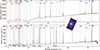 |
Fig. 2. Nuclear (top) and circumnuclear (bottom) averaged spectra obtained from the four channels of MIRI–MRS. The two regions of extraction are delimited by a 1.3″-radius circle (24 pc), as shown on the small inset image (continuum map at 17 μm). This aperture corresponds to 2×FWHM of the PSF at the wavelength of 0–0 S(1) line. The identified emission lines are labeled in different colors. Brackets are omitted from the spectroscopic notation for visual clarity. The H2 rotational lines are labeled in yellow. The main PAH features are indicated with gray vertical bands. Zoomed-in views of the spectra on the different MRS channels are displayed in Appendix C, Figure C.1. |
List of velocity dispersions for every H2 line, obtained via single Gaussian fit.
Line fluxes are listed in Appendix C (Table C.1) for different regions of the FoV. As the lines are spectrally resolved their fluxes were calculated by integrating the continuum-subtracted profiles (shown in Figure C.2 with respective integration boundaries). We applied the aperture correction factors provided by Law et al. (2025) (11–13% for the nucleus and 5% for the larger apertures). For ionized gas lines that have non-single-Gaussian profiles (e.g., asymmetrical or a broad underlying velocity component, such as [NeII] or [ArII]), we find nuclear fluxes 10–15% larger than those computed by single Gaussian fitting (Alonso Herrero et al. 2025), because we are accounting for the underlying broad velocity component.
3.2. Spatial distribution of the molecular gas
The surface-brightness maps of the molecular hydrogen lines 0–0 S(1) and S(5) are presented in Figure 3 (left-side panels), which illustrates the heterogeneous morphology of the gas at different excitation levels4. The maps show diffuse emission, with clumps and filaments spreading over distances on the order of 10 pc, forming a complex disk-like structure. Low excitation H2 is brighter in the ICND, whereas high excitation H2 peaks near the ND.
 |
Fig. 3. Surface-brightness maps (left) and velocity maps (right) of the H2 lines 0–0 S(1) at 17 μm, and S(5) at 6.9 μm, with central spaxels masked due to spectral fringing (see Sect. 2.2). The FWHM of the MRS PSF of the respective channel is shown in the lower right corner. The black contours on the top left map are 8.5 GHz radio VLA contours (0.22, 3.3, and 16 mJy beam−1) from Hardcastle et al. (2003), tracing the jet that aligns with a central cavity seen on the S(1) (note that the VLA beam has a strong north-south elongation). The orange contours on the top left map are 434 μm ALMA CO(6–5) contours (0.01, 0.07, 0.12, 0.18, 0.24, and 0.30 Jy km s−1 beam−1), while those in the bottom left panel are 870 μm ALMA CO(3–2) contours (−0.10, 1.17, 2.45, 3.72, 5.00, and 6.28 Jy km s−1 beam−1) from Espada et al. (2017). CO(6-5) is scarce, and most of CO(3–2) shows large cavities filled by warm H2 emission. The black contours on the bottom left map are JWST IR contours tracing [Ne VI] at 10.51 μm, which features an alignment with the H2 0–0 S(5) hot patches and with the jet. The dashed gray contours on the left maps highlight the two bright hotspots (a) and (b) visible on the S(1) map. The hotspots align with the filaments on the S(5) map and the northern filament visible in CO(3–2) and CO(6–5). The same contours are superimposed in green on the right-hand maps, along with the gray contours tracing the relative surface-brightness maps, and the dashed black line tracing the line of the nodes of the warped-disk model from Neumayer et al. (2007). The contours of the hot S(5) patches aligned with the jet < 20 pc from the AGN are labeled (c) and (d) in the bottom right panel. |
The S(1) map presents two bright hotspots, one north (a) and one south (b) of the AGN. The ND presents a cavity that overlaps the superimposed VLA radio contours of the jet in black (Hardcastle et al. 2003). This alignment suggests that the jet interacts directly with the weakly excited H2.
The S(5) map shows a morphology that is opposite to that of the S(1). The central cavity disappears in favor of two hot patches, (c) and (d), extending for 1″ (18 pc), respectively, north-east and south-west of the AGN (see contour levels in the bottom right panel of Fig. 3). These patches align with the black contours of the [Ne VI] ionized gas line at 10.51 μm, which shows morphological correlation with the jet (Alonso Herrero et al. 2025). The white contours locate the hotspots (a) and (b) of the S(1) map, revealing alignment with the S(5) filaments, especially to the north. The filaments appear to gather into what we define as a spiral streamer (see Sect. 3.3).
Figure 4 provides a schematic of the morphology of the main molecular gas features, consistently with existing literature. The figure also shows the PAH ring studied by Pantoni et al. (2026), which displays the same disky structure of the S(1), with a distinct PAH-deficient area overlapping the (a) hotspot.
 |
Fig. 4. Sub-kiloparsec scale schematic of the center of the Cen A. The straight dotted line represents the direction of the jet. The red semitransparent annulus represents the molecular CND. The black ellipse represents the nuclear ring of CO described by Espada et al. (2017). The brown bars north and south of the AGN represent the filaments of CO(6-5). The blue shape traces the contours of the low dispersion spiral of warm H2 filaments (see Fig. 3 and Fig. 6). The green ellipses represent the S(1) hot spots (a) and (b) (see Fig. 3, upper left). The purple ellipses represent the S(5) hot patches (c) and (d) (see Fig. 3, bottom left). The pink inner empty ring in the center represents the ND of hot gas analyzed by Neumayer et al. (2007). For reference, the dashed-dotted rectangle represents the FoV of CH3. The ICND is the region of the CND covered by our FoV (including H2). The yellow semitransparent annulus represents the PAH ring analyzed by Pantoni et al. (2026). |
The orange contours from ALMA trace the lines of CO(6-5) at 434 μm, on the S(1) panel, and CO(3-2) at 870 μm, on the S(5) panel. The contours show the relative scarcity of cold gas in the FoV, with CO(3-2) presenting large cavities filled by H2. Another possible interpretation of the CO cavities may be flux loss due to low spatial frequency filtering in the SMA and ALMA interferometers.
The CO(6-5) contours show two filaments, respectively north and south of the AGN that intersect the H2 filaments at the location of the hotspots (a) and (b). These bright intersection points have already been presented by Espada et al. (2017), the authors of which describe their emission as shock-driven. CO(6-5) also presents a clump to the east (RA ∼ 3″ from the AGN) that overlaps a faint cavity in H2.
Figure 5 plots the surface-brightness radial profiles of the H2 lines showing the radial gradient of the excitation. H2 emission peaks in the outer regions of the map for S(1) and S(2), halfway through for S(3) and S(4), and near the center for all the other lines from S(5) to S(8).
 |
Fig. 5. Radial profile of mean surface brightness as a function of the projected distance from the AGN. The brightness was averaged within concentric elliptical annuli of ellipticity 0.5 and PA = 155° (following the geometry of the CND). The thickness at the major axis is 0.25″ (4.6 pc) for each annulus. The S(1) and S(2) lines grow brighter farther from the AGN, while lines from the S(5) to S(8) peak near the AGN and grow fainter farther out. |
The masked spaxels at the center of the maps conceal the innermost part of the region analyzed by Neumayer et al. (2007) where SINFONI observations of the H2 1–0 S(1) line at 2.122 μm reveal emissions of hot molecular gas within 3″ (54 pc) of the AGN. Most of the warm H2 in the ICND is hence at the interface between the hot molecular gas of the ND and the cold CO of the CND. This result, along with the radial gradient in the peaking excitation for H2, is consistent with the gradient in the CO(6-5)-to-CO(3-2) flux-density ratio reported by Espada et al. (2017).
3.3. Molecular gas kinematics
The velocity maps for the H2 0–0 S(1) and S(5) lines5 are presented in Figure 3 (right panels). They reveal a global rotation pattern around an axis at PArot ∼ 50°, which is similar to PAjet measured by Neumayer et al. (2007). The line-of-sight velocities range from [ − 180, +110] km s−1 for the S(1)6 to [ − 120, +120] km s−1 for the S(5). For the ionized gas lines such as [Ne II] at 12.837 μm, [Ar II] at 7 μm, and [Fe II] at 5.3 μm, Alonso Herrero et al. (2025) found significant velocity dispersions up to 3 times stronger than H2. Table 1 provides the velocity dispersions for the H2 lines, obtained via a single Gaussian fit, in the full FoV and in the different subregions. The velocity dispersion is corrected for MRS spectral resolution.
We observed noncircular motion components, most notably a characteristic S-shaped distortion, visible in white (close to the systemic velocity) in all H2 velocity maps, already noted by Alonso Herrero et al. (2025). The overlaid contours in Figure 3 trace the level lines from the brightness maps in gray, the (a) and (b) hotspots in green, and the line of the nodes of the warped-disk model from Neumayer et al. (2007) in black. If the hotspots are the result of higher column-density regions due to projection effects on a warped-disk model, we would expect them to align with the line of the nodes. The (a) hotspot from the S(1) map aligns with the redshifted segment of the S-shaped distortion and follows the line of the nodes; however, the (b) hotspot does not show the same alignment. Alonso Herrero et al. (2025) compared the observed velocity field with a 3DBAROLO warped-disk model (Di Teodoro & Fraternali 2015) and found residuals between −40 and 40 km s−1, proving that the warp alone is insufficient to explain the distortion in the velocity field. Therefore, noncircular components must also be present as already concluded by these authors.
Figure 6 shows the velocity-dispersion map of the H2 0–0 S(5) line, which presents a low-velocity-dispersion (FWHM ∼ 70–90 km s−1) spiral structure (20 pc wide) that encompasses the H2 filaments (Fig. 3, left). This coherent low-dispersion structure and the homogeneous surface brightness and H2 excitation (see Sect. 3.4) are features commonly observed in systems where a bulk inflow has been identified (Müller Sánchez et al. 2009; Domínguez-Fernández et al. 2020; Tanaka et al. 2026). For these reasons, we refer to this structure as a spiral streamer.
 |
Fig. 6. Velocity dispersion map of H2 0–0 S(5) line. The green contours trace the (a) and (b) hotspots identified in the S(1) map. The white contours represent the surface brightness of the line, with the (c) and (d) hot patches labeled. The black line indicates the line of the nodes of the warped-disk model from Neumayer et al. (2007). The low-dispersion (70–90 km s−1) spiral streamer overlays the S(5) filaments (white contours) and is consistent with a coherent bulk gas flow. The red ellipses trace the regions where 1D-Gaussian fits of the S(1) and the S(5) reveal residuals > 3σSTD (see Fig. 7). |
Although the rotational H2 line profiles averaged over the entire FoV are well reproduced by single Gaussian components, we note that, locally, the H2 lines exhibit slight asymmetries, particularly in the central regions. Figure 7 presents the spatially averaged line profiles of the 0–0 S(1) and 0–0 S(5) transitions extracted over the full FoV and over two elliptical regions located north and south of the AGN, along the line of nodes of the warped disk (regions highlighted in red in Fig. 6) near the basis of the S-shaped distortion. The profiles show residuals from the single Gaussian fits exceeding the ∼3σSTD level, with deviations centered around −100 and +100 km s−1. This pattern may trace enhanced velocity dispersion resulting from the adiabatic compression of infalling gas onto the central regions of the CND (Vollmer & Davies 2013). Alternatively, it could reflect the presence of a radially outflowing component (Alonso Herrero et al. 2025), possibly arising from inhomogeneous emission within an expanding shell or bubble, where projection effects lead to asymmetric contributions from the approaching and receding sides. Both types of velocity structures are commonly seen in numerical simulations of CNDs (Guo et al. 2024) and in jet-driven outflows (e.g., Mukherjee et al. 2018; Mukherjee 2025) (see discussion in Sect. 4.5).
 |
Fig. 7. H2 0–0 S(1) and S(5) line profiles averaged over the FoV of CH1 (left) and the two elliptical regions located at the base of the S-shaped distortion, as indicated in red in Fig. 6 north (center) and south (right) of the AGN. Uncertainties are highlighted over the plots. The residuals shown beneath each profile trace the deviations from 1D-Gaussian fits with respect to a 3σSTD criterion (horizontal dotted line). Clear deviations are noticeable for both lines at ±100 km s−1, except for the S(5) on the FoV of CH1, where deviations are within the limits. |
3.4. Excitation of the molecular gas
We present our observational results on H2 excitation, comparing different regions, and on a spaxel-by-spaxel basis. The detailed physical modelling of the H2 excitation will be treated in the companion paper II.
3.4.1. Excitation diagrams
We constructed H2 excitation diagrams from the line intensities averaged over three regions (see Table C.1): the FoV of CH1, the ND, and the ICND. We assume that the ND emission is contained in a circle with a 2×FWHM radius. The excitation diagrams, which are shown in Figure 8, display the logarithm of the upper level column densities divided by their statistical weights (degeneracy), log Nu/gu, as a function of the energy of the upper level of the transition in kelvin, Eu/kB. The diagrams show a typical curvature, which is indicative of a distribution of gas temperatures.
 |
Fig. 8. Excitation diagrams for H2 extracted from the averaged cubes, over the full FoV of CH1 (blue), inside (green), and outside (red) a circle of radius 2×FWHM centered around the AGN. The triangles represent the column densities corrected for the OPR. The dashed lines represent the two-temperature linear fits. The S(3) column density is corrected for extinction in the ND via the method presented by Reefe et al. (2025) (see Appendix F). The uncorrected S(3) column density is indicated by the green cross. The deviation of the S(7) from the fit in the ND is due to the difficult de-blending with the [MgVII] line at 5.51 μm. The results of the fits are listed in Table 2. |
We find that the diagrams in the three different regions can be fitted by a simple two-temperature model, and we used the PDRTPY routine to derive temperatures, column densities, and H2 ortho-to-para ratios (Pound & Wolfire 2022). At molecular cloud densities, typically nH = 103 cm−3, the first levels (Ju = 1 − 5) of H2 are thermalized, so they can be used to estimate the total column density, NH2(lin), and the warm gas temperature component, which we find to be within a range of ∼250 − 420 K. The higher levels, Ju > 5, corresponding here to transitions from 0–0 S(4) to S(8), are non-thermalized, and we find excitation temperatures ranging from ∼900 − 1400 K. The routine also corrects column densities of the odd J transitions by fitting the H2 ortho-to-para ratio (OPR). The column density of the Ju = 3 level (corresponding to the S(1) line) over the full FoV is (2.7 − 7.6)×1019 cm−2, so it is well below the critical column density (3.2 × 1025 cm−2 for Ju = 3). The H2 lines are thus optically thin in the ICND.
Estimating the optical depth of the ICND is difficult because the strong mid-IR continuum of the unresolved nucleus outshines part of the ICND, and the 9.7 μm silicate absorption feature is faint. In fitting the Spitzer/IRS spectrum with the PAHFIT tool (Smith & Draine 2012), which assumes a mixing of the dust and the emitting gas, Ogle et al. (2010) estimated an optical depth of 0.5 to 0.8 in the 5–30 μm range, except in the silicate absorption band, near the S(3) line, where it reaches a high value of 2.2. This is an upper limit for the ICND because, as shown in Fig. 2, the silicate absorption feature is located in the ND, and is much less prominent outside. We hence estimated the extinction of the S(3) line in the ND from the S(4)/S(3) line ratios following Reefe et al. (2025), which we explain in Appendix F. We find an optical depth of τ9.7μm = 0.9, which is in agreement with the estimates based on the modeling of the dust continuum (Alexander et al. 1999; Karovska et al. 2003). The S(3) line in the nuclear excitation diagram in Figure 8 (green) is corrected accordingly.
The results of the fits are listed in Table 2, along with the H2 and total gas masses integrated over the respective FoVs for the different regions. These results show heterogeneous excitation among the different observation regions, with excitation temperatures peaking in the ND at ∼420 K for the thermalized levels and almost 1400 K for the higher levels. The OPR is estimated to be around two in the ICND and around three in the ND.
Physical parameters fitted from the excitation diagrams.
The fit yields a total column density for H2 at 300 K around 8.2 × 1020 cm−2 which drops in the ND by a factor of four. This is consistent with the central cavity observed in the S(1) map, since this line traces most of the warm molecular mass.
3.4.2. Spatial variations of H2 temperature and ortho-to-para ratios
We present the warm and hot excitation temperature maps (in K), as well as the OPR map, which were generated using the PDRTPY routine (Pound & Wolfire 2022) on the convolved and reprojected maps, as shown in Figure 9. The two upper panels display the excitation temperature maps. The hot regime map (right) reveals a hot central region surrounding the AGN with excitation temperatures peaking at 1400 K and decreasing outward into the ICND. This morphology identifies the ND where the excitation of H2 is likely driven by UV/X-ray radiation from the AGN (Borkar et al. 2021; Vollmer et al. 2022), with most of the emission arising from higher rotational lines, 0–0 S(4) to S(8) and ro-vibrational line emission (Neumayer et al. 2007). In contrast, the warm regime map (left) shows a colder nuclear cavity, with temperatures in the ICND up to 300 K. The warm map also reveals a warmer region on the eastern (left) side of the disk, with temperatures up to ∼50 K higher than the western side. This region overlaps with the area identified by Alonso Herrero et al. (2025) as showing enhanced [Ne III]/[Ne II] ratios and by Hermosa Muñoz et al. (2025) as exhibiting correlated mid-IR spectral properties, all pointing to distinct physical processes operating there.
 |
Fig. 9. Maps of physical parameters constructed with the PDRTPY routine (Pound & Wolfire 2022) via spaxel-by-spaxel two-linear-component fit of the excitation diagrams: Twarm map of the warm temperature fit component (upper right); Thot map of the hot temperature fit component (upper left); H2 ortho-to-para ratio (OPR) map (bottom left); surface-mass map (bottom right). The maps were convolved to the resolution of the H2 0–0 S(1) map and reprojected to the spaxel grid of CH2. The FoV is limited to the spaxel coverage of the smallest map. The H2 0–0 S(6) and S(8) maps were excluded due to the high number of flagged spaxels. |
The OPR map (bottom left) exhibits pronounced spatial variations across the FoV, with values ranging from 1.6 to 2.4 and never reaching the LTE value of three. The OPR attains its highest values, exceeding 2.2, in the eastern and north-eastern regions, coinciding with the warmer area identified in the temperature map (top left). This side of the map corresponds to the portion of the disk where the jet is oriented toward the observer. In contrast, the ratio decreases below 1.9 in two distinct regions located north and south of the AGN. Notably, the northern low-OPR region overlaps with the (a) hotspot (see Fig. 3).
3.5. Continuum emission and H2-to-continuum ratio
Table 3 provides the luminosity ratio between the mid-IR H2 lines and the monochromatic continuum at 24 μm, to allow a comparison with previous studies (Ogle et al. 2010; Guillard et al. 2012b; Vivian et al. 2022). We computed the continuum luminosity, L24μm, as the specific intensity of the cube at 24 μm; this was integrated over the entire FoV and multiplied by the frequency c/24 μm, where c is the speed of light. The ratio LH2/L24μm presents a difference of almost two orders of magnitude between the ICND and the ND, where the continuum is stronger (see Table 3).
Luminosity ratios between the sum of the mid-IR H2 lines (S(1) to S(8)) and the monochromatic continuum at 24 μm, 17 μm, the PAH7.7μm feature, and the X-ray luminosity (2–10 keV).
Figure 10 presents the spaxel-by-spaxel LS(1)/L17μm luminosity ratio between the H2 0–0 S(1) line and the adjacent monochromatic continuum at 17 μm. We find that this ratio has a strong dependence with the projected distance from the AGN in the innermost part of the CND (< 1.8″ or 30 pc) and then is constant with radius. The radial variation of the LS(1)/L17μm ratio is primarily governed by the continuum intensity, as the S(1) surface brightness varies by less than a factor of two over this distance range. UV PDR models predict a maximum value for the H2-to-PAH7.7μm luminosity ratio of 0.04 (including X-ray pumping) (Guillard et al. 2012b). Given the ratio, LPAH7.7μm/L17μm = 0.1, between the PAH17μm and the continuum at 17 μm averaged over the ICND, we rescaled the PDR limit to 4 × 10⁻³. The total H2-to-17 μm continuum ratio exceeds this limit for all spaxels > 1.3″ (or 24 pc); therefore, we ruled out UV+X-ray heating as the dominant excitation mechanism of the H2 emission in the ICND (see discussion in Sects. 4.1 and 4.2).
 |
Fig. 10. Spaxel-by-spaxel plot of the ratio between the H2 0–0 S(1) luminosity and the monochromatic continuum luminosity νLν at 17 μm (with Lν spectral luminosity). The ratio increases with the projected distance from the AGN up to 30 pc, pointing at a stronger non-radiative excitation of H2 in the outer parts of the ICND. The horizontal dashed line indicates the UV PDR limit from Guillard et al. (2012b) rescaled using the LPAH7.7μm/L17μm ratio of the PAH7.7μm and the continuum at 17 μm (averaged over the ICND). |
We also provide continuum maps in Appendix D (Figure D.1). Table B.1 indicates the spatial FWHM of the centroid of the continuum emission estimated via a 2D-Gaussian fit of the maps. The measured widths are compatible with the expected MRS spatial resolution (Law et al. 2023), suggesting that the emitting source is unresolved.
3.6. Molecular mass gas and dynamical mass
We present our estimate of the total H2 mass. The bottom right panel of Figure 9 shows the surface-density map, in M⊙ pc−2, generated using the PDRTPY routine (Pound & Wolfire 2022). Since the column density is dominated by the lowest energy levels, the map closely resembles the morphology of the 0-0 S(1) line, with hotspots (a) and (b) clearly visible, and bearing, respectively, 30% and 20% of the whole mass, while the eastern region shows a column density almost one order of magnitude lower than that of the hotspots. From this map, we integrated a total molecular hydrogen mass of MH2(map) = 8.1 × 10⁴ M⊙ over a FoV of 19.8 arcsec2. This result is consistent with the mass MH2(lin) = 1.4 × 10⁵ M⊙ obtained from the linear fit of the excitation diagrams reported in Table 2 for the FoV of CH1, once we account for the fact that the FoV of the surface density map is 40% smaller due to flagged spaxels. A comparison with the cold mass gas estimate from Espada et al. (2017) is provided in Section 4.4.
Since the S(0) line is outside the MRS spectral coverage, the mass estimate from the two-linear-component fit of the excitation diagram is limited to the ∼300 K warm gas. We used the H2Powerlaw7 tool from Togi & Smith (2016) to perform a power-law fit of the excitation diagrams to extrapolate the mass of H2 to lower temperatures. The power-law fits are presented in Appendix E, Figure E.1. These fits estimate the mass MH2(pow) for H2 to the lower fitting temperatures, Tlow, of 110 K in the nucleus and 60 K in the ICND. Since H2 does not radiate in IR at 60 K, we increased the lower limit of the fit, Tlow, to 100 K, and hence find a mass MH2(100K) about five times lower than MH2(pow) in the ICND. These results are listed in Table 2.
Figure 11 shows the position–velocity (PV) diagram extracted along the line of the nodes defined by the warped-disk model from Neumayer et al. (2007). We followed the line of the nodes to ideally maximize the projected line-of-sight bulk velocity component. The wavelength solution calibration of Argyriou et al. (2023) through the MRS wavelength range was used to compute the uncertainties on velocities. Due to masking of the central spaxels in our maps, we were unable to trace the gas dynamics within the black hole’s sphere of influence, which is marked by the vertical blue lines at 0.8″ (15 pc) from the center (Neumayer et al. 2007).
 |
Fig. 11. PV diagrams of H2 gas extracted from the rotational line velocity maps. The path chosen follows the line of the nodes of the warped-disk model from Neumayer et al. (2007) to maximize the projected velocity component. The small quadrant shows the S(1) velocity map with the path of extraction for reference. Every point in the diagram is averaged on a square of nine spaxels (120 pc2) following the black line. A typical 1σ error bar of 30 km s−1 is given on the right. The dashed blue lines represent the expected radius of influence of the SMBH given the mass estimated by Neumayer et al. (2007). |
Assuming a Newtonian approximation, the dynamical mass enclosed within a sphere of radius r is given by
![Mathematical equation: $$ \begin{aligned} M_\mathrm{dyn} = \frac{r}{G} \left[\frac{V}{ \cos (i)}\right]^2\ ,\end{aligned} $$](/articles/aa/full_html/2026/07/aa58362-25/aa58362-25-eq4.gif) (1)
(1)
where G is the gravitational constant, V is the projected line-of-sight velocity, and i is the inclination angle. We adopted a radius of r ∼ 4″ and estimated V as the average S(1) velocity in the radial interval between 3.5″ and 4.5″. Position angle values were taken from Neumayer et al. (2007) and span around a median of PAnodes ∼ 155°. This yields a dynamical mass of (5 ± 0.4)×108 M⊙. Such estimate encompasses the contributions from H2, stellar mass, and the central SMBH.
4. Discussion
4.1. High H2-to-dust IR emission ratio: Possible evidence for shock excitation
We discuss here how the results that we present can be interpreted as indicators of different sources of excitation. Ogle et al. (2007, 2010) defined an empirical threshold of LH2/L24μm = 0.02 between H2 line emission and continuum at 24 μm to classify galaxies that present significant non-radiative heating of the gas (so-called MOHEGs). The results presented in Section 3.5 show that this limit is exceeded in all regions studied in this work except the nuclear region. Ogle et al. (2010) revisited this criterion, as it does not account for the variation in AGN contribution to the continuum emission, and the authors proposed the ratio LH2/LPAH7.7μm as a much better tracer of the relative contribution of mechanical heating with respect to radiative heating. Table 3 presents the ratios computed from the PAH7.7μm flux provided by Pantoni et al. (2026) using PAHDecomp (Donnan et al. 2023, 2024). The ratio is above the limit of 0.04 expected from PDR models (Guillard et al. 2012b) in all regions. Although the PAH feature in the ND does not emerge clearly from the continuum, we estimate a LH2/LPAH7.7μm ratio in the ICND that is four times higher compared to the ND. This is consistent with Israel et al. (2017), which found shock-excited gas at < 1000 K from the 1–0 S(J) line ratios observed by Herschel. Such ratios strongly suggest that collisional excitation from shocks in the ICND provides a major source of molecular hydrogen excitation.
Espada et al. (2017) supported the same conclusion for CO, indicating the non-axisymmetric morpho-kinematics and the resulting torque exerted on the gas as possible causes of loss of angular momentum. The same argument can be extended to the non-axisymmetric, H2 morpho-kinematical features, reinforcing the importance of shocks in energy and angular-momentum dissipation for the molecular gas.
Strong H2-to-PAH ratios have been observed in 3C 293 by Riffel et al. (2025) and in IC5063 by Dasyra et al. (2024) and will be discussed for other radio-loud AGNs by Riffel et al, in prep, particularly in regions where the velocity dispersion is high (up to ∼500 km s−1).
4.2. H2 emission from dissipation of turbulent mechanical energy
We first examine the role of turbulent heating in maintaining the observed H2 emission. Following Guillard et al. (2012a), the turbulent heating rate required us to maintain the H2 luminosity, which can be estimated from the energy dissipation rate and is expressed as the luminosity-to-mass ratio LH2/MH2, where MH2 is the mass of H2 at 300 K. If the emission is entirely powered by turbulent dissipation, the following relation holds:
 (2)
(2)
where the left-hand side of the equation is the turbulent heating rate (Mac Low 1999), σT the turbulent velocity dispersion, and l the characteristic size of the region over which the dispersion is measured.
Ogle et al. (2010) reported dissipation rates between 1 and 33 L⊙/M⊙ for their sample of MOHEGs. Over the CH1 FoV, we derived, for Centaurus A, a dissipation rate of LH2/MH2(lin) = 4.43 L⊙/M⊙; therefore, within the MOHEG range. Adopting lFoV = 4.5″, corresponding to the width of the FoV in CH1, we inferred a turbulent velocity dispersion (FWHM) of 270 km s−1 required to sustain the observed H2 emission. This is 40% higher than the observed mean velocity dispersion (see Table 1). However, at the scale of the FoV, the complex gas kinematics and disk geometry make it difficult to quantitatively isolate the turbulence from the rotational and radial bulk flow components in the velocity-dispersion field.
Locally, at the PSF scale lPSF, we can identify regions where the rotational component is small, especially close to the minor kinematic axis along the H2 filaments. Here the turbulent motions dominate the velocity field. Assuming lPSF = 0.3″ (6 pc), corresponding to the PSF size in CH1, we computed the turbulent heating rate for velocity dispersions between 70 and 90 km s−1, as observed along the coherent spiral streamer in the S(5) dispersion map (Fig. 6). This yields turbulent heating rates of 1.7 and 2.6 L⊙/M⊙, respectively. Over the same lPSF = 0.3″ aperture along the spiral streamer, we measured a luminosity-to-mass ratio of  . At the 10 pc scale, the dissipation rate thus matches the estimated turbulent heating rate, suggesting that the dissipation of mechanical turbulent energy significantly contributes to the excitation of the molecular gas. This is in agreement with theoretical models and observations of the CND in the galactic center of NGC 1068 (Vollmer et al. 2022).
4.3. X-ray heating and CR heating of the H2 gas
We discuss the impact of X-ray photons from the AGN corona and of CR on H2 excitation. Using X-ray-dominated-region (XDR) models (Maloney et al. 1996), Ogle et al. (2010) estimated a maximum H2-to-X-ray luminosity ratio of LH2/LX(2 − 10 keV) ≲ 0.01 in X-ray-dominated environments. This value assumes that all the X-ray flux is absorbed by the XDR and that the fraction of the absorbed X-ray flux that goes into gas heating by photoelectrons is high (40%), but it could be a factor of two lower. The Chandra X-ray luminosity of the central, unresolved, point-source is LX(2 − 10 keV) = 5.01 × 1041 erg s−1 (Ogle et al. 2010). Given Chandra’s PSF profile (Kraft et al. 2002), less than 30% of LX(2 − 10 keV) can come from the ICND (within 1.3″ or 24 pc of the AGN). This yields a LH2/LX(2 − 10 keV) ratio of 0.001 (lower limit) in the ND and 0.013 (upper limit) in the ICND. The former ratio is below the upper threshold of the XDR models, while the latter exceeds it, which suggests that radiative heating dominates in the ND, while additional heating mechanisms are required in the ICND; this is consistent with the results shown in Figure 10. A detailed modeling of the contribution of XDRs to the H2 line emission is out of the scope of this paper.
For CR heating of the H2 gas, we can estimate the ionization rate ζ required to sustain the H2 line emission. Assuming an ionization energy of 4 eV per ionized molecule (MEUDON code, Le Petit et al. 2006), given the mass of an H2 molecule, mH2, and based on the luminosity-mass ratio, we find ζ = mH2 (LH2/MH2(lin)) / 4eV ∼ 4.5 × 10⁻¹² s−1. This result is five orders of magnitude higher than the typical ionization rate in the Milky Way (Shaw et al. 2006), one order of magnitude above the average found by Ogle et al. (2010) for MOHEGs, and more than two orders of magnitude above the ionization rate observed in the central molecular zone of the Galactic center (Ravikularaman et al. 2025). CR heating is thus unlikely to be the main powering source of the H2 line emission over the scale of Cen A’s ICND.
4.4. Comparison of total molecular gas mass with Spitzer and ALMA
We compared our gas-mass estimates with those from previous studies. Using Spitzer observations integrated within a 13.7 arcsec2 FoV, Ogle et al. (2010) derived a total H2 column density of 5 × 1021 cm−2 by fitting the excitation diagram with three temperature components based on transitions from S(0) to S(7). Their result, rescaled to the MIRI FoV (CH1), assuming a homogeneous distribution, yields a total mass of 1.1 × 10⁶ M⊙ for the ∼150 K component in the excitation diagram, which is consistent with our estimate of Mgas(100K) ∼ 0.8 × 10⁶ M⊙. From CO observations, Espada et al. (2017) reported a total gas mass of 9 × 10⁷ M⊙ over a much larger FoV of 144 arcsec2. We extracted the flux of the C0(3-2) line, integrating over their ALMA map, which is restricted to the region covered by the MIRI FoV (CH1). Using the same conversion factor of 0.1 they use between the CO(1-0) and the CO(3-2) lines and a factor XCO = 4 × 1020 cm−2 K km s−1 (for the nuclear region of Cen A Israel et al. 2014; Miura et al. 2021), we find a total gas mass of 1.7×10⁶ M⊙. This result is about two times larger compared to our Mgas(100K) estimate. This discrepancy may be due to an overestimated XCO factor or the fact that ALMA observations probe gas that is colder than 100 K, which we do not detect with MRS.
4.5. Comparison between H2 and the ionized gas
Several results highlight morphological and kinematical differences between H2 and the ionized gas. The ionized line emissions peak in a cone-like structure aligned with the jet (Alonso Herrero et al. 2025), whereas H2 emission is more diffuse across the ICND. As shown in Figure 3 (bottom left panel), we find similar contrasts between the [Ne VI] and H2 morphologies; the [Ne VI] emission is concentrated around the AGN and extended along the jet axis, with no trace of the low-dispersion filamentary structures observed in H2. The elongated morphology of the [O IV] and [Ne V] lines perpendicularly to the ICND and indicative of an outflow was also noted by Quillen et al. (2008), from Spitzer/IRS observations.
The morpho-kinematics of H2 present similarities with the CO filaments forming the CND in Cen A (analyzed by Espada et al. 2017), and at larger kiloparsec scales with filaments of inflowing CO in NGC 1275 (Salomé et al. 2011; Lim et al. 2008). These filamentary structures are morphologically consistent with simulations of magnetized accreting molecular gas (M87★, Guo et al. 2024), which also predict secondary magnetically driven polar outflows of molecular gas, although these are less significant. The H2 low dispersion spiral structure and the radial excitation gradient (see Fig. 6 and D.2) point to a similar scenario.
The morpho-kinematics of the ionized gas are analyzed in detail in the companion paper Alonso Herrero et al. (2025) and point to an outflow in the form of an expanding bubble driven by the jet, similar to those seen in AGN jet simulations (Mukherjee 2025). Although a molecular outflow is detected at larger scales (> 15″ or 280 pc from the nucleus Israel et al. 2017), we only detect slight deviations in the wings of the H2 lines in the inner disk (see Sect. 3.3 and Fig. 7). This pattern may trace enhanced velocity dispersion resulting from the adiabatic compression of infalling gas onto the central regions of the CND (Vollmer & Davies 2013). Alternatively, it could reflect the presence of a radially outflowing component (Alonso Herrero et al. 2025), possibly arising from inhomogeneous emission within an expanding shell or bubble, where projection effects lead to asymmetric contributions from the approaching and receding sides.
Both types of velocity structure are commonly seen in numerical simulations of CNDs (Guo et al. 2024) and in jet-driven outflows (e.g., Mukherjee et al. 2018; Mukherjee 2025). However, without a more detailed modeling of the velocity fields and line profiles, it is not possible at this stage to distinguish between inflows and outflows in the H2 kinematics.
Overall, H2 lines exhibit velocity dispersions about one order of magnitude lower compared to the ionized gas. The Gaussian-fit sigma maps from Alonso Herrero et al. (2025) reveal that the velocity dispersion for the ionized gas is maximal in the ND, within ∼1.5″ of the AGN, and decreases along the jet. This net different behavior between the two phases has already been reported for other sources (i.e., NGC 1275, Riffel et al. 2020) and is thought to be caused by different gas density and dynamical coupling to the jet (Morganti et al. 2015; Mukherjee et al. 2016; Speranza et al. 2022).
5. Conclusions
We obtained parsec-scale resolution mid-IR spectral maps of the 100–200 pc innermost region of Cen A with the JWST/MRS, covering the 5–28 μm wavelength range. This work, along with two companion papers on Cen A (Alonso Herrero et al. 2025; Pantoni et al. 2026) are part of the MIRI GTO program MICONIC. We focused here on spatially resolved morpho-kinematics and excitation of the H2 rotational line emission. Our main results are the following:
-
The H2 surface brightness maps show an inhomogeneous morphology with filaments of molecular gas peaking in the ICND at lower excitation and near the AGN at stronger excitation; lower levels also reveal a central cavity (40 pc in diameter).
-
Velocity maps show global rotation plus a warped-disk geometry and noncircular motions. The filaments display lower dispersion, which is consistent with a coherent inflow toward the AGN, while residuals from Gaussian fits suggest a possible outflow at the base (see Alonso Herrero et al. 2025). The molecular gas exhibits different morpho-kinematics from the ionized component, which peaks near the AGN and along the jet, showing higher dispersion and outflow signatures.
-
Excitation diagrams indicate that the average temperatures of the bulk of the H2 are ∼2 times higher in the nucleus (416±12) K than in the ICND (286 ± 7) K. The physical parameter maps show temperatures up to 340 K on the eastern ICND side, where the jet is pointed toward us. The filaments contain most of the molecular mass and show the lowest ortho-to-para ratio (∼1.8).
-
The mass of the molecular gas obtained via a fitting of the excitation diagram at 100 K is (9.6 ± 4)×105 M⊙ in the inner disk, while the dynamical mass is (5 ± 0.4)×108 M⊙ within 4″ (74 pc) of the AGN.
-
The LH2/L17μm ratio increases by two orders of magnitude from the ND to the ICND and exceeds the threshold of photoionization processes at 1.3″ (30 pc) from the AGN, indicating collisional excitation in the ICND. The H2/PAH7.7μm luminosity ratio exceeds the PDR model threshold for significant non-radiative excitation in all regions.
-
The S(5) velocity dispersion at the PSF scale (6 pc) yields heating rates consistent with the dissipation rate LH2/MH2 = 2.7 L⊙/M⊙ measured along the coherent spiral streamer, supporting that dissipation of mechanical energy contributes to the excitation of H2.
-
The ratio LH2/LX(2 − 10 keV) exceeds by a factor 4 the upper limit predicted by XDR models, again supporting the importance of shocks in heating the H2 gas.
The last three points in particular are further evidence of the importance of shocks in heating H2 and in causing loss of angular momentum in the CND, as already suggested in existing literature (Espada et al. 2017; Ogle et al. 2010). A forthcoming analysis presented in paper II will combine radiative and mechanical excitation models–based on the methodology presented in Villa-Vélez et al. (2024)–to quantify, on a spaxel-by-spaxel basis, the relative contributions of shocks, UV, and X-ray pumping to H2 excitation, disentangling the gas energy budget of the ICND.
Acknowledgments
This work is based, in part, on observations made with the NASA/ESA/CSA James Webb Space Telescope. PG acknowledges the Sorbonne University (FSI), the Centre National d’Etudes Spatiales (CNES), the ‘Programme National de Cosmologie and Galaxies’ (PNCG) and the ‘Physique Chimie du Milieu Interstellaire’ (PCMI) programs of CNRS/INSU, with INC/INP co-funded by CEA and CNES, for there financial supports. AAH and LHM acknowledge support from grant PID2021-124665NB-I00 funded by MCIN/AEI/10.13039/501100011033 and by ERDF A way of making Europe. LP and MB acknowledge funding from the Belgian Science Policy Office (BELSPO) through the PRODEX project “JWST/MIRI Science exploitation” (C4000142239). RAR acknowledges the support from the Conselho Nacional de Desenvolvimento Científico e Tecnológico (CNPq; Projects 303450/2022-3, and 403398/2023-1), the Coordenação de Aperfeiçoamento de Pessoal de Nível Superior (CAPES; Project 88887.894973/2023-00), and Fundação de Amparo à Pesquisa do Estado do Rio Grande do Sul (FAPERGS; Project 25/2551-0002765-9)
References
- Alexander, D. M., Efstathiou, A., Hough, J. H., et al. 1999, MNRAS, 310, 78 [Google Scholar]
- Alonso Herrero, A., Hermosa Muñoz, L., Labiano, A., et al. 2024, A&A, 690, A95 [NASA ADS] [CrossRef] [EDP Sciences] [Google Scholar]
- Alonso Herrero, A., Hermosa Muñoz, L., Labiano, A., et al. 2025, A&A, 699, A334 [NASA ADS] [CrossRef] [EDP Sciences] [Google Scholar]
- Álvarez Márquez, J., Labiano, A., Guillard, P., et al. 2023, A&A, 672, A108 [NASA ADS] [CrossRef] [EDP Sciences] [Google Scholar]
- Argyriou, I., Glasse, A., Law, D. R., et al. 2023, A&A, 675, A111 [NASA ADS] [CrossRef] [EDP Sciences] [Google Scholar]
- Argyriou, I., Lage, C., Rieke, G. H., et al. 2023, A&A, 680, A96 [NASA ADS] [CrossRef] [EDP Sciences] [Google Scholar]
- Borkar, A., Adhikari, T. P., Różańska, A., et al. 2021, MNRAS, 500, 3536 [Google Scholar]
- Buiten, V. A., van der Werf, P. P., Viti, S., et al. 2025, A&A, 699, A312 [Google Scholar]
- Bushouse, H. 2020, in Astronomical Data Analysis Software and Systems XXIX, eds. R. Pizzo, E. R. Deul, J. D. Mol, J. de Plaa, & H. Verkouter, ASP Conf. Ser., 527, 583 [NASA ADS] [Google Scholar]
- Capelo, P. R., Feruglio, C., Hickox, R. C., & Tombesi, F. 2023, Handbook of X-ray and Gamma-ray Astrophysics (Springer Living Reference Work), 126 [Google Scholar]
- Combes, F. 2001, in Advanced Lectures on the Starburst-AGN, eds. I. Aretxaga, D. Kunth, & R. Mújica, 223 [Google Scholar]
- Dasyra, K. M., Paraschos, G. F., Combes, F., et al. 2024, ApJ, 977, 156 [Google Scholar]
- Di Teodoro, E. M., & Fraternali, F. 2015, MNRAS, 451, 3021 [Google Scholar]
- Domínguez-Fernández, A. J., Alonso-Herrero, A., García-Burillo, S., et al. 2020, A&A, 643, A127 [NASA ADS] [CrossRef] [EDP Sciences] [Google Scholar]
- Donnan, F. R., García-Bernete, I., Rigopoulou, D., et al. 2023, MNRAS, 519, 3691 [CrossRef] [Google Scholar]
- Donnan, F. R., García-Bernete, I., Rigopoulou, D., et al. 2024, MNRAS, 529, 1386 [NASA ADS] [CrossRef] [Google Scholar]
- Espada, D., Matsushita, S., Peck, A., et al. 2009, ApJ, 695, 116 [Google Scholar]
- Espada, D., Matsushita, S., Miura, R. E., et al. 2017, ApJ, 843, 136 [NASA ADS] [CrossRef] [Google Scholar]
- Espada, D., Verley, S., Miura, R. E., et al. 2019, ApJ, 887, 88 [Google Scholar]
- Fanaroff, B. L., & Riley, J. M. 1974, MNRAS, 167, 31P [Google Scholar]
- Gasman, D., Argyriou, I., Sloan, G. C., et al. 2023, A&A, 673, A102 [NASA ADS] [CrossRef] [EDP Sciences] [Google Scholar]
- Gasman, D., Argyriou, I., Morrison, J. E., et al. 2024, A&A, 688, A226 [NASA ADS] [CrossRef] [EDP Sciences] [Google Scholar]
- Gasman, D., Argyriou, I., Law, D. R., et al. 2025, A&A, 697, A58 [NASA ADS] [CrossRef] [EDP Sciences] [Google Scholar]
- Guillard, P., Boulanger, F., Pineau des Forêts, G., et al. 2012a, ApJ, 749, 158 [NASA ADS] [CrossRef] [Google Scholar]
- Guillard, P., Ogle, P. M., Emonts, B. H. C., et al. 2012b, ApJ, 747, 95 [NASA ADS] [CrossRef] [Google Scholar]
- Guo, M., Stone, J. M., Quataert, E., & Kim, C.-G. 2024, ApJ, 973, 141 [Google Scholar]
- Haardt, F., & Maraschi, L. 1991, ApJ, 380, L51 [Google Scholar]
- Hardcastle, M. J., Worrall, D. M., Kraft, R. P., et al. 2003, ApJ, 593, 169 [NASA ADS] [CrossRef] [Google Scholar]
- Harris, G. L. H., Rejkuba, M., & Harris, W. E. 2010, PASA, 27, 457 [NASA ADS] [CrossRef] [Google Scholar]
- Hermosa Muñoz, L., Alonso-Herrero, A., Labiano, A., et al. 2025, A&A, 693, A321 [NASA ADS] [CrossRef] [EDP Sciences] [Google Scholar]
- Israel, F. P. 1998, A&A Rev., 8, 237 [Google Scholar]
- Israel, F. P., Güsten, R., Meijerink, R., et al. 2014, A&A, 562, A96 [NASA ADS] [CrossRef] [EDP Sciences] [Google Scholar]
- Israel, F. P., Güsten, R., Meijerink, R., Requena-Torres, M. A., & Stutzki, J. 2017, A&A, 599, A53 [NASA ADS] [CrossRef] [EDP Sciences] [Google Scholar]
- Karovska, M., Marengo, M., Elvis, M., et al. 2003, ApJ, 598, L91 [Google Scholar]
- Kraft, R. P., Forman, W. R., Jones, C., et al. 2002, ApJ, 569, 54 [Google Scholar]
- Kraft, R. P., Hardcastle, M. J., Forman, W. R., et al. 2003, New Astron. Rev., 47, 625 [Google Scholar]
- Labiano, A., Azzollini, R., Bailey, J., et al. 2016, in Observatory Operations: Strategies, Processes, and Systems VI, eds. A. B. Peck, R. L. Seaman, & C. R. Benn, SPIE Conf. Ser., 9910, 99102W [Google Scholar]
- Labiano, A., Argyriou, I., Álvarez Márquez, J., et al. 2021, A&A, 656, A57 [NASA ADS] [CrossRef] [EDP Sciences] [Google Scholar]
- Law, D. R., Morrison, J. E., Argyriou, I., et al. 2023, AJ, 166, 45 [NASA ADS] [CrossRef] [Google Scholar]
- Law, D. R., Argyriou, I., Gordon, K. D., et al. 2025, AJ, 169, 67 [Google Scholar]
- Le Petit, F., Nehmé, C., Le Bourlot, J., & Roueff, E. 2006, ApJS, 164, 506 [NASA ADS] [CrossRef] [Google Scholar]
- Lim, J., Ao, Y., & Dinh-V-Trung, 2008, ApJ, 672, 252 [NASA ADS] [CrossRef] [Google Scholar]
- Lusso, E., Hennawi, J. F., Comastri, A., et al. 2013, ApJ, 777, 86 [Google Scholar]
- Mac Low, M.-M. 1999, ApJ, 524, 169 [Google Scholar]
- Maloney, P. R., Hollenbach, D. J., & Tielens, A. G. G. M. 1996, ApJ, 466, 561 [Google Scholar]
- Miura, R. E., Espada, D., Hirota, A., et al. 2021, MNRAS, 504, 6198 [NASA ADS] [CrossRef] [Google Scholar]
- Morganti, R., Oosterloo, T., Oonk, J. B. R., Frieswijk, W., & Tadhunter, C. 2015, A&A, 580, A1 [NASA ADS] [CrossRef] [EDP Sciences] [Google Scholar]
- Morrison, J. E., Dicken, D., Argyriou, I., et al. 2023, PASP, 135, 075004 [NASA ADS] [CrossRef] [Google Scholar]
- Mukherjee, D. 2025, Galaxies, 13, 102 [Google Scholar]
- Mukherjee, D., Bicknell, G. V., Sutherland, R., & Wagner, A. 2016, MNRAS, 461, 967 [NASA ADS] [CrossRef] [Google Scholar]
- Mukherjee, D., Bicknell, G. V., Wagner, A. Y., Sutherland, R. S., & Silk, J. 2018, MNRAS, 479, 5544 [NASA ADS] [CrossRef] [Google Scholar]
- Müller Sánchez, F., Davies, R. I., Genzel, R., et al. 2009, ApJ, 691, 749 [Google Scholar]
- Neumayer, N. 2007, Ph.D. Thesis, Max Planck Institute [Google Scholar]
- Neumayer, N., Cappellari, M., Reunanen, J., et al. 2007, ApJ, 671, 1329 [NASA ADS] [CrossRef] [Google Scholar]
- Ogle, P. M., Antonucci, R., Appleton, P. N., et al. 2007, in AAS Meeting Abstracts, 211, 97.21 [Google Scholar]
- Ogle, P., Boulanger, F., Guillard, P., et al. 2010, ApJ, 724, 1193 [NASA ADS] [CrossRef] [Google Scholar]
- Pantoni, L., Baes, M., Decin, L., et al. 2026, A&A, 709, A237 [NASA ADS] [CrossRef] [EDP Sciences] [Google Scholar]
- Patapis, P., Argyriou, I., Law, D. R., et al. 2024, A&A, 682, A53 [NASA ADS] [CrossRef] [EDP Sciences] [Google Scholar]
- Pontoppidan, K. M., Salyk, C., Banzatti, A., et al. 2024, ApJ, 963, 158 [NASA ADS] [CrossRef] [Google Scholar]
- Pound, M. W., & Wolfire, M. G. 2022, AJ, 165, 25 [Google Scholar]
- Quillen, A. C., Graham, J. R., & Frogel, J. A. 1993, ApJ, 412, 550 [NASA ADS] [CrossRef] [Google Scholar]
- Quillen, A. C., Brookes, M. H., Keene, J., et al. 2006, ApJ, 645, 1092 [Google Scholar]
- Quillen, A. C., Bland-Hawthorn, J., Green, J. D., et al. 2008, MNRAS, 384, 1469 [NASA ADS] [CrossRef] [Google Scholar]
- Quillen, A. C., Neumayer, N., Oosterloo, T., & Espada, D. 2010, PASA, 27, 396 [Google Scholar]
- Ravikularaman, S., Recchia, S., Phan, V. H. M., & Gabici, S. 2025, A&A, 694, A114 [NASA ADS] [CrossRef] [EDP Sciences] [Google Scholar]
- Reefe, M., McDonald, M., Chatzikos, M., et al. 2025, ApJ, 989, 156 [Google Scholar]
- Riffel, R. A., Storchi-Bergmann, T., Zakamska, N. L., & Riffel, R. 2020, MNRAS, 496, 4857 [NASA ADS] [CrossRef] [Google Scholar]
- Riffel, R. A., Souza-Oliveira, G. L., Costa-Souza, J. H., et al. 2025, ApJ, 982, 69 [Google Scholar]
- Salomé, P., Combes, F., Revaz, Y., et al. 2011, A&A, 531, A85 [NASA ADS] [CrossRef] [EDP Sciences] [Google Scholar]
- Salomé, Q., Salomé, P., Combes, F., Hamer, S., & Heywood, I. 2016, A&A, 586, A45 [NASA ADS] [CrossRef] [EDP Sciences] [Google Scholar]
- Shaw, G., Ferland, G. J., Srianand, R., & Abel, N. P. 2006, ApJ, 639, 941 [Google Scholar]
- Smith, J. D., & Draine, B. 2012, Astrophysics Source Code Library [record ascl:1210.009] [Google Scholar]
- Speranza, G., Ramos Almeida, C., Acosta-Pulido, J. A., et al. 2022, A&A, 665, A55 [NASA ADS] [CrossRef] [EDP Sciences] [Google Scholar]
- Tanaka, K., Nagai, M., & Kamegai, K. 2026, ApJ, 999, 185 [Google Scholar]
- Togi, A., & Smith, J. D. T. 2016, ApJ, 830, 18 [NASA ADS] [CrossRef] [Google Scholar]
- Veilleux, S., Maiolino, R., Bolatto, A. D., & Aalto, S. 2020, A&A Rev., 28, 2 [NASA ADS] [CrossRef] [Google Scholar]
- Villa-Vélez, J. A., Godard, B., Guillard, P., & Pineau des Forêts, G. 2024, A&A, 688, A96 [NASA ADS] [CrossRef] [EDP Sciences] [Google Scholar]
- Vivian, U., Lai, T., Bianchin, M., et al. 2022, ApJ, 940, L5 [NASA ADS] [CrossRef] [Google Scholar]
- Vollmer, B., & Davies, R. I. 2013, A&A, 556, A31 [NASA ADS] [CrossRef] [EDP Sciences] [Google Scholar]
- Vollmer, B., Davies, R. I., Gratier, P., et al. 2022, A&A, 665, A102 [NASA ADS] [CrossRef] [EDP Sciences] [Google Scholar]
- Weiß, A., Kovács, A., Güsten, R., et al. 2008, A&A, 490, 77 [NASA ADS] [CrossRef] [EDP Sciences] [Google Scholar]
- Wells, M., Pel, J.-W., Glasse, A., et al. 2015, PASP, 127, 646 [NASA ADS] [CrossRef] [Google Scholar]
- Wright, G. S., Rieke, G. H., Glasse, A., et al. 2023, PASP, 135, 048003 [NASA ADS] [CrossRef] [Google Scholar]
This is acceptable given the strong brightness of the target over the whole FoV.
The skewness in the S(1) velocity field is localized to a narrow, blueshifted region in the southeastern corner of the map, at the limit of the FoV.
Appendix A: MRS spatial and spectral resolutions
We summarize here the technical specifications for each MRS channel and sub-channel. Table A.2 details the FoV opening and centering, as well as the spatial and spectral resolutions and samplings. To estimate the spatial resolution as the FWHM of the PSF at the observation wavelength, we use the PSF characterization equation provided by Law et al. (2023):
![Mathematical equation: $$ \begin{aligned} \mathrm{FWHM} _{\mathrm{PSF} }\left[ \mathrm{arcsec} \right]=0.033^{\prime \prime } \times \lambda \left[\mu \mathrm{m} \right]\,+0.106^{\prime \prime } \end{aligned} $$](/articles/aa/full_html/2026/07/aa58362-25/aa58362-25-eq7.gif) (A.1)
(A.1)
To estimate the spectral resolution power at different wavelengths we use the characterization equation provided by Pontoppidan et al. (2024):
![Mathematical equation: $$ \begin{aligned} R(\lambda ) = \frac{\lambda }{\Delta \lambda } = K_1 \ + \ K_2\ \times \ \lambda [\mu m ] \end{aligned} $$](/articles/aa/full_html/2026/07/aa58362-25/aa58362-25-eq8.gif) (A.2)
(A.2)
where the factors K1 and K2 depend on the channels and the sub-channels and are reported in Table A.1.
Coefficients for Eq. A.2 for the resolution power, by channel and sub-channel.
MRS technical specs.
Appendix B: Continuum measurements
We present in Table B.1 the results of the 2D-Gaussian fit of the centroid of the continuum emission (see Sect. 3.5), along with photometric measurements of the continuum, over each channel’s FoV and in the ND.
Results of the 2D-gaussian fit of the continuum maps and measurements of the continuum fluxes close to the H2 lines.
Appendix C: Spectral extractions and line fluxes
We present in Figure C.1 the ND and the ICND spectra of Cen A from the four MRS channels. Extractions are performed respectively inside and outside a 1.3"-radius (24 pc) circle centered on the AGN. This aperture corresponds to 2×FWHM of the PSF at 17 μm. The extraction regions are displayed in Figure 2. In Figure C.2 we present the line profiles extracted by averaging over the full FoV of the continuum subtracted sub-cubes. The black vertical lines mark the integration boundaries set to calculate the line fluxes listed in Table C.1 (see Sect. 3.1).
 |
Fig. C.1. Spectrum of the inner region of Centaurus A. Zooms on the different MRS channels comparing the ND with the ICND, respectively inside and outside a 1.3"-radius circle (24 pc), as shown on the small inset image (continuum map at 17 μm) of Fig 2. This aperture corresponds to 2×FWHM of the PSF at the 0–0 S(1) line. |
 |
Fig. C.2. Continuum-subtracted line profiles averaged over the respective channel’s full FoV. The black vertical bars represent the flux integration boundaries for each line. The [SIII], [NeIII], [NeII], [ArII], [ArIII], [NeVI], [MgV] are assumed to have Lorentzian profiles, and hence are wider compared to the other lines. Notice that [ClII], [NaIII], and [NiII] present a strongly noisy continuum, which renders the fit of the profile challenging. |
Line fluxes extracted over different areas.
Appendix D: Continuum and spectral maps
We present here all the generated maps for H2 and for the continuum. Figure D.1 shows the maps of the continuum near each of the H2 lines. Figures D.2, D.3, and D.4 show all the H2 maps respectively of moment-0, 1, and 2. Details are provided in the main text. For the H2 0–0 S(8), we only show the moment maps generated with the 1σSTD spaxel flagging criterion since this method recovers spaxels in the ICND that reveal morphological correlations with the other maps.
 |
Fig. D.1. Continuum maps extracted around the H2 rotational lines (with the line masked). The red-star symbol marks the position of the central AGN: in RA-Dec 13:25:27.63 -43:01:08.30 (J2000). |
 |
Fig. D.2. H2 rotational line surface brightness maps in [W m−2 sr−1] for all transitions from 0–0 S(1) to S(8). Central spaxels are masked. Spaxels with undetected lines are replaced with background noise level. The figures reveal how the brighter spots spiral towards the AGN along the H2 filaments (white contours in Fig 6), as excitation becomes stronger. |
 |
Fig. D.3. Velocity maps in [km s−1]. Central spaxels and no-line-detection spaxels are masked. The maps show clear signs of global rotation, along with an evident S-shaped distortion due to the warped-disk geometry of the CND plus non-circular motion. |
 |
Fig. D.4. Velocity dispersion maps in [km s−1]. Central spaxels and no-line-detection spaxels are masked. |
Appendix E: Power-law fits of the excitation diagrams
We present here the power-law fits of the excitation diagrams performed using the H2powerlaw tool by Togi & Smith (2016), over the FoV of CH1, the ND, and the ICND. The tool fits the H2 lines assuming a continuous temperature distribution following the relation:
 (E.1)
(E.1)
where dN is the column density between T and T + dT, n is the power-law index, and m is a constant. Integrating E.1 between two temperature bounds Tlow and Tupp, and assuming that T is equal to the rotational temperature, m is found to be:
 (E.2)
(E.2)
where Ntot is the total H2 column density in the FoV. Above 1000 K, Togi & Smith (2016) indicate that Tupp has a negligible impact on the mass estimate and it is hence fixed by default at 2000 K. The parameters Tlow and n are adjusted to fit the column densities from the excitation diagram, allowing to calculate Ntot and thus, given the mass of one H2 molecule mH2, the FoV surface angle Ω, and the distance from the source d, the total H2 mass is Mtot = mH2NtotΩd2.
Figure E.1 shows the results of the power-law fits on our H2 excitation diagrams, over the full FoV, the ND, and the ICND.
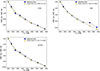 |
Fig. E.1. Power-law fit of the excitation diagrams, performed using the H2Powerlaw tool from Togi & Smith (2016) on the fluxes extracted from the averaged cubes, over the full FoV of CH1, inside (ND), and outside (ICND) a circle centered around the AGN of radius 2×FWHM. The legends report the results of the fit: n is the slope of the power-law, while Tl is the lower temperature limit of the fit Tlow. The S(3) line in the ND is corrected for extinction via the method presented by Reefe et al. (2025) (see App. F). The deviation of the S(7) from the fit in the ND is due to the difficult de-blending of the [MgVII] line at 5.51 μm. |
Appendix F: Absorption in the silicate band
Ogle et al. (2010) use a continuum fit to estimate absorption and find a non-negligible 0.4 relative extinction in the silicate band, near the H2 0–0 S(3) line at 9.68 μm. We present here the method we used to estimate the optical depth τ9.7μm, based on Reefe et al. (2025).
We mask the S(3) line in the excitation diagrams and perform a power-law fit (see App. E) to infer the intrinsic S(3) emission from the other lines. Flux ratios between the i-th and the j-th lines are expected to follow the relation:
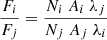 (F.1)
(F.1)
were Fi, Ni, Ai, and λi are respectively the flux, the column density, the Einstein coefficient, and the wavelenght of the i-th line. The next H2 line adjacent S(3) is S(4) which is out of the silicate band. We hence compare the intrinsic flux ratio [FS(4)/FS(3)]intrinsic inferred from the fit of the excitation diagram, with the observed ratio [FS(4)/FS(3)]observed. The optical depth at 9.68 μm is therefore estimated as:
![Mathematical equation: $$ \begin{aligned} \tau _{9.7\mu \mathrm m} = \mathrm{ln} \left(\frac{[F_\mathrm{S(4)} /F_\mathrm{S(3)} ]_\mathrm{observed} }{[F_\mathrm{S(4)} /F_\mathrm{S(3)} ]_\mathrm{intrinsic} }\right) \end{aligned} $$](/articles/aa/full_html/2026/07/aa58362-25/aa58362-25-eq12.gif) (F.2)
(F.2)
We use this result to correct the S(3) line flux in our nuclear excitation diagram.
All Tables
List of velocity dispersions for every H2 line, obtained via single Gaussian fit.
Luminosity ratios between the sum of the mid-IR H2 lines (S(1) to S(8)) and the monochromatic continuum at 24 μm, 17 μm, the PAH7.7μm feature, and the X-ray luminosity (2–10 keV).
Coefficients for Eq. A.2 for the resolution power, by channel and sub-channel.
Results of the 2D-gaussian fit of the continuum maps and measurements of the continuum fluxes close to the H2 lines.
All Figures
|
Fig. 1. Zoomed-in view of the inner region of Centaurus A adapted from Espada et al. (2017). Left: Color composite image of Centaurus A. Credit: ESO/WFI - Optical; MPIfR/ESO/APEX/Weiß et al. (2008) – Submillimeter; NASA/CXC/CfA/Kraft et al. (2003) – X-ray. Center: integrated CO(2-1) emission map from SMA (green) (Espada et al. 2009); dust emission at 8 μm from Spitzer/IRAC (blue) (Quillen et al. 2006); the jet in X-ray from Chandra (red) (Kraft et al. 2003). Right: Integrated CO(3-2) and CO(6-5) maps from ALMA (green and blue, respectively); H2 1–0 S(1) map at 2.122 μm from VLT/SINFONI (red). The red rectangles in the right panel are the mosaic footprints of the four MRS channels. The dashed white ellipses outline the CND as defined by Espada et al. (2017). |
| In the text | |
|
Fig. 2. Nuclear (top) and circumnuclear (bottom) averaged spectra obtained from the four channels of MIRI–MRS. The two regions of extraction are delimited by a 1.3″-radius circle (24 pc), as shown on the small inset image (continuum map at 17 μm). This aperture corresponds to 2×FWHM of the PSF at the wavelength of 0–0 S(1) line. The identified emission lines are labeled in different colors. Brackets are omitted from the spectroscopic notation for visual clarity. The H2 rotational lines are labeled in yellow. The main PAH features are indicated with gray vertical bands. Zoomed-in views of the spectra on the different MRS channels are displayed in Appendix C, Figure C.1. |
| In the text | |
|
Fig. 3. Surface-brightness maps (left) and velocity maps (right) of the H2 lines 0–0 S(1) at 17 μm, and S(5) at 6.9 μm, with central spaxels masked due to spectral fringing (see Sect. 2.2). The FWHM of the MRS PSF of the respective channel is shown in the lower right corner. The black contours on the top left map are 8.5 GHz radio VLA contours (0.22, 3.3, and 16 mJy beam−1) from Hardcastle et al. (2003), tracing the jet that aligns with a central cavity seen on the S(1) (note that the VLA beam has a strong north-south elongation). The orange contours on the top left map are 434 μm ALMA CO(6–5) contours (0.01, 0.07, 0.12, 0.18, 0.24, and 0.30 Jy km s−1 beam−1), while those in the bottom left panel are 870 μm ALMA CO(3–2) contours (−0.10, 1.17, 2.45, 3.72, 5.00, and 6.28 Jy km s−1 beam−1) from Espada et al. (2017). CO(6-5) is scarce, and most of CO(3–2) shows large cavities filled by warm H2 emission. The black contours on the bottom left map are JWST IR contours tracing [Ne VI] at 10.51 μm, which features an alignment with the H2 0–0 S(5) hot patches and with the jet. The dashed gray contours on the left maps highlight the two bright hotspots (a) and (b) visible on the S(1) map. The hotspots align with the filaments on the S(5) map and the northern filament visible in CO(3–2) and CO(6–5). The same contours are superimposed in green on the right-hand maps, along with the gray contours tracing the relative surface-brightness maps, and the dashed black line tracing the line of the nodes of the warped-disk model from Neumayer et al. (2007). The contours of the hot S(5) patches aligned with the jet < 20 pc from the AGN are labeled (c) and (d) in the bottom right panel. |
| In the text | |
|
Fig. 4. Sub-kiloparsec scale schematic of the center of the Cen A. The straight dotted line represents the direction of the jet. The red semitransparent annulus represents the molecular CND. The black ellipse represents the nuclear ring of CO described by Espada et al. (2017). The brown bars north and south of the AGN represent the filaments of CO(6-5). The blue shape traces the contours of the low dispersion spiral of warm H2 filaments (see Fig. 3 and Fig. 6). The green ellipses represent the S(1) hot spots (a) and (b) (see Fig. 3, upper left). The purple ellipses represent the S(5) hot patches (c) and (d) (see Fig. 3, bottom left). The pink inner empty ring in the center represents the ND of hot gas analyzed by Neumayer et al. (2007). For reference, the dashed-dotted rectangle represents the FoV of CH3. The ICND is the region of the CND covered by our FoV (including H2). The yellow semitransparent annulus represents the PAH ring analyzed by Pantoni et al. (2026). |
| In the text | |
|
Fig. 5. Radial profile of mean surface brightness as a function of the projected distance from the AGN. The brightness was averaged within concentric elliptical annuli of ellipticity 0.5 and PA = 155° (following the geometry of the CND). The thickness at the major axis is 0.25″ (4.6 pc) for each annulus. The S(1) and S(2) lines grow brighter farther from the AGN, while lines from the S(5) to S(8) peak near the AGN and grow fainter farther out. |
| In the text | |
|
Fig. 6. Velocity dispersion map of H2 0–0 S(5) line. The green contours trace the (a) and (b) hotspots identified in the S(1) map. The white contours represent the surface brightness of the line, with the (c) and (d) hot patches labeled. The black line indicates the line of the nodes of the warped-disk model from Neumayer et al. (2007). The low-dispersion (70–90 km s−1) spiral streamer overlays the S(5) filaments (white contours) and is consistent with a coherent bulk gas flow. The red ellipses trace the regions where 1D-Gaussian fits of the S(1) and the S(5) reveal residuals > 3σSTD (see Fig. 7). |
| In the text | |
|
Fig. 7. H2 0–0 S(1) and S(5) line profiles averaged over the FoV of CH1 (left) and the two elliptical regions located at the base of the S-shaped distortion, as indicated in red in Fig. 6 north (center) and south (right) of the AGN. Uncertainties are highlighted over the plots. The residuals shown beneath each profile trace the deviations from 1D-Gaussian fits with respect to a 3σSTD criterion (horizontal dotted line). Clear deviations are noticeable for both lines at ±100 km s−1, except for the S(5) on the FoV of CH1, where deviations are within the limits. |
| In the text | |
|
Fig. 8. Excitation diagrams for H2 extracted from the averaged cubes, over the full FoV of CH1 (blue), inside (green), and outside (red) a circle of radius 2×FWHM centered around the AGN. The triangles represent the column densities corrected for the OPR. The dashed lines represent the two-temperature linear fits. The S(3) column density is corrected for extinction in the ND via the method presented by Reefe et al. (2025) (see Appendix F). The uncorrected S(3) column density is indicated by the green cross. The deviation of the S(7) from the fit in the ND is due to the difficult de-blending with the [MgVII] line at 5.51 μm. The results of the fits are listed in Table 2. |
| In the text | |
|
Fig. 9. Maps of physical parameters constructed with the PDRTPY routine (Pound & Wolfire 2022) via spaxel-by-spaxel two-linear-component fit of the excitation diagrams: Twarm map of the warm temperature fit component (upper right); Thot map of the hot temperature fit component (upper left); H2 ortho-to-para ratio (OPR) map (bottom left); surface-mass map (bottom right). The maps were convolved to the resolution of the H2 0–0 S(1) map and reprojected to the spaxel grid of CH2. The FoV is limited to the spaxel coverage of the smallest map. The H2 0–0 S(6) and S(8) maps were excluded due to the high number of flagged spaxels. |
| In the text | |
|
Fig. 10. Spaxel-by-spaxel plot of the ratio between the H2 0–0 S(1) luminosity and the monochromatic continuum luminosity νLν at 17 μm (with Lν spectral luminosity). The ratio increases with the projected distance from the AGN up to 30 pc, pointing at a stronger non-radiative excitation of H2 in the outer parts of the ICND. The horizontal dashed line indicates the UV PDR limit from Guillard et al. (2012b) rescaled using the LPAH7.7μm/L17μm ratio of the PAH7.7μm and the continuum at 17 μm (averaged over the ICND). |
| In the text | |
|
Fig. 11. PV diagrams of H2 gas extracted from the rotational line velocity maps. The path chosen follows the line of the nodes of the warped-disk model from Neumayer et al. (2007) to maximize the projected velocity component. The small quadrant shows the S(1) velocity map with the path of extraction for reference. Every point in the diagram is averaged on a square of nine spaxels (120 pc2) following the black line. A typical 1σ error bar of 30 km s−1 is given on the right. The dashed blue lines represent the expected radius of influence of the SMBH given the mass estimated by Neumayer et al. (2007). |
| In the text | |
|
Fig. C.1. Spectrum of the inner region of Centaurus A. Zooms on the different MRS channels comparing the ND with the ICND, respectively inside and outside a 1.3"-radius circle (24 pc), as shown on the small inset image (continuum map at 17 μm) of Fig 2. This aperture corresponds to 2×FWHM of the PSF at the 0–0 S(1) line. |
| In the text | |
|
Fig. C.2. Continuum-subtracted line profiles averaged over the respective channel’s full FoV. The black vertical bars represent the flux integration boundaries for each line. The [SIII], [NeIII], [NeII], [ArII], [ArIII], [NeVI], [MgV] are assumed to have Lorentzian profiles, and hence are wider compared to the other lines. Notice that [ClII], [NaIII], and [NiII] present a strongly noisy continuum, which renders the fit of the profile challenging. |
| In the text | |
|
Fig. D.1. Continuum maps extracted around the H2 rotational lines (with the line masked). The red-star symbol marks the position of the central AGN: in RA-Dec 13:25:27.63 -43:01:08.30 (J2000). |
| In the text | |
|
Fig. D.2. H2 rotational line surface brightness maps in [W m−2 sr−1] for all transitions from 0–0 S(1) to S(8). Central spaxels are masked. Spaxels with undetected lines are replaced with background noise level. The figures reveal how the brighter spots spiral towards the AGN along the H2 filaments (white contours in Fig 6), as excitation becomes stronger. |
| In the text | |
|
Fig. D.3. Velocity maps in [km s−1]. Central spaxels and no-line-detection spaxels are masked. The maps show clear signs of global rotation, along with an evident S-shaped distortion due to the warped-disk geometry of the CND plus non-circular motion. |
| In the text | |
|
Fig. D.4. Velocity dispersion maps in [km s−1]. Central spaxels and no-line-detection spaxels are masked. |
| In the text | |
|
Fig. E.1. Power-law fit of the excitation diagrams, performed using the H2Powerlaw tool from Togi & Smith (2016) on the fluxes extracted from the averaged cubes, over the full FoV of CH1, inside (ND), and outside (ICND) a circle centered around the AGN of radius 2×FWHM. The legends report the results of the fit: n is the slope of the power-law, while Tl is the lower temperature limit of the fit Tlow. The S(3) line in the ND is corrected for extinction via the method presented by Reefe et al. (2025) (see App. F). The deviation of the S(7) from the fit in the ND is due to the difficult de-blending of the [MgVII] line at 5.51 μm. |
| In the text | |
Current usage metrics show cumulative count of Article Views (full-text article views including HTML views, PDF and ePub downloads, according to the available data) and Abstracts Views on Vision4Press platform.
Data correspond to usage on the plateform after 2015. The current usage metrics is available 48-96 hours after online publication and is updated daily on week days.
Initial download of the metrics may take a while.