


| Issue |
A&A
Volume 711, July 2026
|
|
|---|---|---|
| Article Number | A156 | |
| Number of page(s) | 20 | |
| Section | Cosmology (including clusters of galaxies) | |
| DOI | https://doi.org/10.1051/0004-6361/202557590 | |
| Published online | 13 July 2026 | |
Euclid Quick Data Release (Q1)
XXXVII. Searching for giant gravitational arcs in galaxy clusters with mask region-based convolutional neural networks
1
Dipartimento di Fisica e Scienze della Terra, Università degli Studi di Ferrara, Via Giuseppe Saragat 1, 44122 Ferrara, Italy
2
INAF-Osservatorio di Astrofisica e Scienza dello Spazio di Bologna, Via Piero Gobetti 93/3, 40129 Bologna, Italy
3
INAF-Osservatorio Astronomico di Capodimonte, Via Moiariello 16, 80131 Napoli, Italy
4
Dipartimento di Fisica “Aldo Pontremoli”, Università degli Studi di Milano, Via Celoria 16, 20133 Milano, Italy
5
INFN-Sezione di Bologna, Viale Berti Pichat 6/2, 40127 Bologna, Italy
6
Instituto de Física de Cantabria, Edificio Juan Jordá, Avenida de los Castros, 39005 Santander, Spain
7
INAF-IASF Milano, Via Alfonso Corti 12, 20133 Milano, Italy
8
Universita di Salerno, Dipartimento di Fisica “E.R. Caianiello”, Via Giovanni Paolo II 132, I-84084 Fisciano (SA), Italy
9
Institute of Cosmology and Gravitation, University of Portsmouth, Portsmouth PO1 3FX, UK
10
INFN – Gruppo Collegato di Salerno – Sezione di Napoli, Dipartimento di Fisica “E.R. Caianiello”, Universita di Salerno, Via Giovanni Paolo II, 132, I-84084 Fisciano (SA), Italy
11
ESAC/ESA, Camino Bajo del Castillo, s/n, Urb. Villafranca del Castillo, 28692 Villanueva de la Cañada, Madrid, Spain
12
INAF-Osservatorio Astronomico di Brera, Via Brera 28, 20122 Milano, Italy
13
IFPU, Institute for Fundamental Physics of the Universe, Via Beirut 2, 34151 Trieste, Italy
14
INAF-Osservatorio Astronomico di Trieste, Via G. B. Tiepolo 11, 34143 Trieste, Italy
15
INFN, Sezione di Trieste, Via Valerio 2, 34127 Trieste TS, Italy
16
SISSA, International School for Advanced Studies, Via Bonomea 265, 34136 Trieste TS, Italy
17
Dipartimento di Fisica e Astronomia, Università di Bologna, Via Gobetti 93/2, 40129 Bologna, Italy
18
INAF-Osservatorio Astronomico di Padova, Via dell’Osservatorio 5, 35122 Padova, Italy
19
Dipartimento di Fisica, Università di Genova, Via Dodecaneso 33, 16146 Genova, Italy
20
INFN-Sezione di Genova, Via Dodecaneso 33, 16146 Genova, Italy
21
Department of Physics “E. Pancini”, University Federico II, Via Cinthia 6, 80126 Napoli, Italy
22
Dipartimento di Fisica, Università degli Studi di Torino, Via P. Giuria 1, 10125 Torino, Italy
23
INFN-Sezione di Torino, Via P. Giuria 1, 10125 Torino, Italy
24
INAF-Osservatorio Astrofisico di Torino, Via Osservatorio 20, 10025 Pino Torinese (TO), Italy
25
European Space Agency/ESTEC, Keplerlaan 1, 2201 AZ, Noordwijk, The Netherlands
26
Leiden Observatory, Leiden University, Einsteinweg 55, 2333 CC, Leiden, The Netherlands
27
Centro de Investigaciones Energéticas, Medioambientales y Tecnológicas (CIEMAT), Avenida Complutense 40, 28040 Madrid, Spain
28
Port d’Informació Científica, Campus UAB, C. Albareda s/n, 08193 Bellaterra (Barcelona), Spain
29
INAF-Osservatorio Astronomico di Roma, Via Frascati 33, 00078 Monteporzio Catone, Italy
30
INFN Section of Naples, Via Cinthia 6, 80126 Napoli, Italy
31
Dipartimento di Fisica e Astronomia “Augusto Righi” – Alma Mater Studiorum Università di Bologna, Viale Berti Pichat 6/2, 40127 Bologna, Italy
32
Instituto de Astrofísica de Canarias, E-38205 La Laguna, Tenerife, Spain
33
Institute for Astronomy, University of Edinburgh, Royal Observatory, Blackford Hill, Edinburgh EH9 3HJ, UK
34
European Space Agency/ESRIN, Largo Galileo Galilei 1, 00044 Frascati, Roma, Italy
35
Université Claude Bernard Lyon 1, CNRS/IN2P3, IP2I Lyon, UMR 5822, Villeurbanne F-69100, France
36
Aix-Marseille Université, CNRS, CNES, LAM, Marseille, France
37
Institut de Ciències del Cosmos (ICCUB), Universitat de Barcelona (IEEC-UB), Martí i Franquès 1, 08028 Barcelona, Spain
38
Institució Catalana de Recerca i Estudis Avançats (ICREA), Passeig de Lluís Companys 23, 08010 Barcelona, Spain
39
Institut de Ciencies de l’Espai (IEEC-CSIC), Campus UAB, Carrer de Can Magrans, s/n Cerdanyola del Vallés, 08193 Barcelona, Spain
40
UCB Lyon 1, CNRS/IN2P3, IUF, IP2I Lyon, 4 Rue Enrico Fermi, 69622 Villeurbanne, France
41
Mullard Space Science Laboratory, University College London, Holmbury St Mary, Dorking, Surrey RH5 6NT, UK
42
Departamento de Física, Faculdade de Ciências, Universidade de Lisboa, Edifício C8, Campo Grande, PT1749-016 Lisboa, Portugal
43
Instituto de Astrofísica e Ciências do Espaço, Faculdade de Ciências, Universidade de Lisboa, Campo Grande, 1749-016 Lisboa, Portugal
44
Department of Astronomy, University of Geneva, Ch. d’Ecogia 16, 1290 Versoix, Switzerland
45
Université Paris-Saclay, CNRS, Institut d’Astrophysique Spatiale, 91405 Orsay, France
46
INFN-Padova, Via Marzolo 8, 35131 Padova, Italy
47
Aix-Marseille Université, CNRS/IN2P3, CPPM, Marseille, France
48
Max Planck Institute for Extraterrestrial Physics, Giessenbachstr. 1, 85748 Garching, Germany
49
Universitäts-Sternwarte München, Fakultät für Physik, Ludwig-Maximilians-Universität München, Scheinerstr. 1, 81679 München, Germany
50
INAF-Istituto di Astrofisica e Planetologia Spaziali, Via del Fosso del Cavaliere, 100, 00100 Roma, Italy
51
Space Science Data Center, Italian Space Agency, Via del Politecnico snc, 00133 Roma, Italy
52
INFN-Bologna, Via Irnerio 46, 40126 Bologna, Italy
53
University Observatory, LMU Faculty of Physics, Scheinerstr. 1, 81679 Munich, Germany
54
INFN-Sezione di Milano, Via Celoria 16, 20133 Milano, Italy
55
Institute of Theoretical Astrophysics, University of Oslo, P.O. Box 1029 Blindern 0315, Oslo, Norway
56
Jet Propulsion Laboratory, California Institute of Technology, 4800 Oak Grove Drive, Pasadena, CA 91109, USA
57
Department of Physics, Lancaster University, Lancaster LA1 4YB, UK
58
Felix Hormuth Engineering, Goethestr. 17, 69181 Leimen, Germany
59
Technical University of Denmark, Elektrovej 327, 2800 Kgs. Lyngby, Denmark
60
Cosmic Dawn Center (DAWN), Denmark
61
Max-Planck-Institut für Astronomie, Königstuhl 17, 69117 Heidelberg, Germany
62
NASA Goddard Space Flight Center, Greenbelt, MD 20771, USA
63
Department of Physics and Astronomy, University College London, Gower Street, London WC1E 6BT, UK
64
Department of Physics and Helsinki Institute of Physics, Gustaf Hällströmin katu 2, University of Helsinki, 00014 Helsinki, Finland
65
Université Paris-Saclay, Université Paris Cité, CEA, CNRS, AIM, 91191 Gif-sur-Yvette, France
66
Université de Genève, Département de Physique Théorique and Centre for Astroparticle Physics, 24 quai Ernest-Ansermet, CH-1211 Genève 4, Switzerland
67
Department of Physics, P.O. Box 64, University of Helsinki, 00014 Helsinki, Finland
68
Helsinki Institute of Physics, Gustaf Hällströmin katu 2, University of Helsinki, 00014 Helsinki, Finland
69
Kapteyn Astronomical Institute, University of Groningen, PO Box 800, 9700 AV, Groningen, The Netherlands
70
Laboratoire d’etude de l’Univers et des phenomenes eXtremes, Observatoire de Paris, Université PSL, Sorbonne Université, CNRS, 92190 Meudon, France
71
SKAO, Jodrell Bank, Lower Withington, Macclesfield SK11 9FT, UK
72
Centre de Calcul de l’IN2P3/CNRS, 21 Avenue Pierre de Coubertin, 69627 Villeurbanne Cedex, France
73
Universität Bonn, Argelander-Institut für Astronomie, Auf dem Hügel 71, 53121 Bonn, Germany
74
INFN-Sezione di Roma, Piazzale Aldo Moro, 2 – c/o Dipartimento di Fisica, Edificio G. Marconi, 00185 Roma, Italy
75
Dipartimento di Fisica e Astronomia “Augusto Righi” – Alma Mater Studiorum Università di Bologna, Via Piero Gobetti 93/2, 40129 Bologna, Italy
76
Department of Physics, Institute for Computational Cosmology, Durham University, South Road, Durham DH1 3LE, UK
77
Université Paris Cité, CNRS, Astroparticule et Cosmologie, 75013 Paris, France
78
CNRS-UCB International Research Laboratory, Centre Pierre Binétruy, IRL2007, CPB-IN2P3, Berkeley, USA
79
University of Applied Sciences and Arts of Northwestern Switzerland, School of Engineering, 5210 Windisch, Switzerland
80
Institut d’Astrophysique de Paris, 98 bis Boulevard Arago, 75014 Paris, France
81
Institut d’Astrophysique de Paris, UMR 7095, CNRS, and Sorbonne Université, 98 bis Boulevard Arago, 75014 Paris, France
82
Institute of Physics, Laboratory of Astrophysics, Ecole Polytechnique Fédérale de Lausanne (EPFL), Observatoire de Sauverny, 1290 Versoix, Switzerland
83
Telespazio UK S.L. for European Space Agency (ESA), Camino bajo del Castillo, s/n, Urbanizacion Villafranca del Castillo, Villanueva de la Cañada, 28692, Madrid, Spain
84
Institut de Física d’Altes Energies (IFAE), The Barcelona Institute of Science and Technology, Campus UAB, 08193 Bellaterra (Barcelona), Spain
85
DARK, Niels Bohr Institute, University of Copenhagen, Jagtvej 155, 2200 Copenhagen, Denmark
86
Waterloo Centre for Astrophysics, University of Waterloo, Waterloo, Ontario N2L 3G1, Canada
87
Department of Physics and Astronomy, University of Waterloo, Waterloo, Ontario N2L 3G1, Canada
88
Perimeter Institute for Theoretical Physics, Waterloo, Ontario N2L 2Y5, Canada
89
Centre National d’Etudes Spatiales – Centre Spatial de Toulouse, 18 Avenue Edouard Belin, 31401 Toulouse Cedex 9, France
90
Institute of Space Science, Str. Atomistilor, Nr. 409 Măgurele, Ilfov 077125, Romania
91
Dipartimento di Fisica e Astronomia “G. Galilei”, Università di Padova, Via Marzolo 8, 35131 Padova, Italy
92
Institut für Theoretische Physik, University of Heidelberg, Philosophenweg 16, 69120 Heidelberg, Germany
93
Institut de Recherche en Astrophysique et Planétologie (IRAP), Université de Toulouse, CNRS, UPS, CNES, 14 Av. Edouard Belin, 31400 Toulouse, France
94
Université St Joseph; Faculty of Sciences, Beirut, Lebanon
95
Departamento de Física, FCFM, Universidad de Chile, Blanco Encalada 2008, Santiago, Chile
96
Universität Innsbruck, Institut für Astro- und Teilchenphysik, Technikerstr. 25/8, 6020 Innsbruck, Austria
97
Institut d’Estudis Espacials de Catalunya (IEEC), Edifici RDIT, Campus UPC, 08860 Castelldefels, Barcelona, Spain
98
Satlantis, University Science Park, Sede Bld 48940, Leioa-Bilbao, Spain
99
Institute of Space Sciences (ICE, CSIC), Campus UAB, Carrer de Can Magrans, s/n, 08193 Barcelona, Spain
100
Instituto de Astrofísica e Ciências do Espaço, Faculdade de Ciências, Universidade de Lisboa, Tapada da Ajuda, 1349-018 Lisboa, Portugal
101
Cosmic Dawn Center (DAWN)
102
Niels Bohr Institute, University of Copenhagen, Jagtvej 128, 2200 Copenhagen, Denmark
103
Universidad Politécnica de Cartagena, Departamento de Electrónica y Tecnología de Computadoras, Plaza del Hospital 1, 30202 Cartagena, Spain
104
Infrared Processing and Analysis Center, California Institute of Technology, Pasadena, CA 91125, USA
105
Istituto Nazionale di Fisica Nucleare, Sezione di Ferrara, Via Giuseppe Saragat 1, 44122 Ferrara, Italy
106
INAF, Istituto di Radioastronomia, Via Piero Gobetti 101, 40129 Bologna, Italy
107
Astronomical Observatory of the Autonomous Region of the Aosta Valley (OAVdA), Loc. Lignan 39, I-11020 Nus (Aosta Valley), Italy
108
Université Côte d’Azur, Observatoire de la Côte d’Azur, CNRS, Laboratoire Lagrange, Bd de l’Observatoire, CS 34229, 06304 Nice Cedex 4, France
109
Aurora Technology for European Space Agency (ESA), Camino bajo del Castillo, s/n, Urbanizacion Villafranca del Castillo, Villanueva de la Cañada, 28692, Madrid, Spain
110
ICL, Junia, Université Catholique de Lille, LITL, 59000 Lille, France
111
ICSC – Centro Nazionale di Ricerca in High Performance Computing, Big Data e Quantum Computing, Via Magnanelli 2, Bologna, Italy
112
Instituto de Física Teórica UAM-CSIC, Campus de Cantoblanco, 28049 Madrid, Spain
113
CERCA/ISO, Department of Physics, Case Western Reserve University, 10900 Euclid Avenue, Cleveland, OH 44106, USA
114
Technical University of Munich, TUM School of Natural Sciences, Physics Department, James-Franck-Str. 1, 85748 Garching, Germany
115
Max-Planck-Institut für Astrophysik, Karl-Schwarzschild-Str. 1, 85748 Garching, Germany
116
Laboratoire Univers et Théorie, Observatoire de Paris, Université PSL, Université Paris Cité, CNRS, 92190 Meudon, France
117
Departamento de Física Fundamental, Universidad de Salamanca, Plaza de la Merced s/n, 37008 Salamanca, Spain
118
IRFU, CEA, Université Paris-Saclay, 91191 Gif-sur-Yvette Cedex, France
119
Université de Strasbourg, CNRS, Observatoire Astronomique de Strasbourg, UMR 7550, 67000 Strasbourg, France
120
Center for Data-Driven Discovery, Kavli IPMU (WPI), UTIAS, The University of Tokyo, Kashiwa, Chiba 277-8583, Japan
121
Max-Planck-Institut für Physik, Boltzmannstr. 8, 85748 Garching, Germany
122
Dipartimento di Fisica – Sezione di Astronomia, Università di Trieste, Via Tiepolo 11, 34131 Trieste, Italy
123
Jodrell Bank Centre for Astrophysics, Department of Physics and Astronomy, University of Manchester, Oxford Road, Manchester M13 9PL, UK
124
California Institute of Technology, 1200 E California Blvd, Pasadena, CA 91125, USA
125
SCITAS, Ecole Polytechnique Fédérale de Lausanne (EPFL), 1015 Lausanne, Switzerland
126
Department of Physics & Astronomy, University of California Irvine, Irvine, CA 92697, USA
127
Department of Mathematics and Physics E. De Giorgi, University of Salento, Via per Arnesano, CP-I93, 73100 Lecce, Italy
128
INFN, Sezione di Lecce, Via per Arnesano, CP-193, 73100 Lecce, Italy
129
INAF-Sezione di Lecce, c/o Dipartimento Matematica e Fisica, Via per Arnesano, 73100 Lecce, Italy
130
Departamento Física Aplicada, Universidad Politécnica de Cartagena, Campus Muralla del Mar, 30202 Cartagena, Murcia, Spain
131
Observatorio Nacional, Rua General Jose Cristino, 77-Bairro Imperial de Sao Cristovao, Rio de Janeiro, 20921-400, Brazil
132
CEA Saclay, DFR/IRFU, Service d’Astrophysique, Bat. 709, 91191 Gif-sur-Yvette, France
133
Department of Astronomy, University of Florida, Bryant Space Science Center, Gainesville, FL 32611, USA
134
Department of Computer Science, Aalto University, PO Box 15400 Espoo FI-00 076, Finland
135
Instituto de Astrofísica de Canarias, E-38205 La Laguna; Universidad de La Laguna, Dpto. Astrofísica, E-38206 La Laguna, Tenerife, Spain
136
Caltech/IPAC, 1200 E. California Blvd., Pasadena, CA 91125, USA
137
Ruhr University Bochum, Faculty of Physics and Astronomy, Astronomical Institute (AIRUB), German Centre for Cosmological Lensing (GCCL), 44780 Bochum, Germany
138
Department of Physics and Astronomy, Vesilinnantie 5, University of Turku, 20014 Turku, Finland
139
Serco for European Space Agency (ESA), Camino bajo del Castillo, s/n, Urbanizacion Villafranca del Castillo, Villanueva de la Cañada, 28692, Madrid, Spain
140
ARC Centre of Excellence for Dark Matter Particle Physics, Melbourne, Australia
141
Centre for Astrophysics & Supercomputing, Swinburne University of Technology, Hawthorn, Victoria 3122, Australia
142
Department of Physics and Astronomy, University of the Western Cape, Bellville, Cape Town, 7535, South Africa
143
Department of Physics, Oxford University, Keble Road, Oxford OX1 3RH, UK
144
DAMTP, Centre for Mathematical Sciences, Wilberforce Road, Cambridge CB3 0WA, UK
145
Kavli Institute for Cosmology Cambridge, Madingley Road, Cambridge CB3 0HA, UK
146
Department of Astrophysics, University of Zurich, Winterthurerstrasse 190, 8057 Zurich, Switzerland
147
Department of Physics, Centre for Extragalactic Astronomy, Durham University, South Road, Durham DH1 3LE, UK
148
Institute for Theoretical Particle Physics and Cosmology (TTK), RWTH Aachen University, 52056 Aachen, Germany
149
Oskar Klein Centre for Cosmoparticle Physics, Department of Physics, Stockholm University, Stockholm SE-106 91, Sweden
150
Astrophysics Group, Blackett Laboratory, Imperial College London, London SW7 2AZ, UK
151
Univ. Grenoble Alpes, CNRS, Grenoble INP, LPSC-IN2P3, 53, Avenue des Martyrs, 38000 Grenoble, France
152
INAF-Osservatorio Astrofisico di Arcetri, Largo E. Fermi 5, 50125 Firenze, Italy
153
Dipartimento di Fisica, Sapienza Università di Roma, Piazzale Aldo Moro 2, 00185 Roma, Italy
154
Centro de Astrofísica da Universidade do Porto, Rua das Estrelas, 4150-762 Porto, Portugal
155
Instituto de Astrofísica e Ciências do Espaço, Universidade do Porto, CAUP, Rua das Estrelas, PT4150-762 Porto, Portugal
156
HE Space for European Space Agency (ESA), Camino bajo del Castillo, s/n, Urbanizacion Villafranca del Castillo, Villanueva de la Cañada, 28692, Madrid, Spain
157
INAF – Osservatorio Astronomico d’Abruzzo, Via Maggini, 64100 Teramo, Italy
158
Theoretical Astrophysics, Department of Physics and Astronomy, Uppsala University, Box 516, 751 37 Uppsala, Sweden
159
Institute for Astronomy, University of Hawaii, 2680 Woodlawn Drive, Honolulu, HI 96822, USA
160
Mathematical Institute, University of Leiden, Einsteinweg 55, 2333 CA, Leiden, The Netherlands
161
Institute of Astronomy, University of Cambridge, Madingley Road, Cambridge CB3 0HA, UK
162
Univ. Lille, CNRS, Centrale Lille, UMR 9189 CRIStAL, 59000 Lille, France
163
Department of Astrophysical Sciences, Peyton Hall, Princeton University, Princeton, NJ 08544, USA
164
Space Physics and Astronomy Research Unit, University of Oulu, Pentti Kaiteran katu 1, FI-90014 Oulu, Finland
165
Center for Computational Astrophysics, Flatiron Institute, 162 5th Avenue, 10010 New York, NY, USA
166
Department of Physics and Astronomy, University of British Columbia, Vancouver, BC V6T 1Z1, Canada
★ Corresponding author: This email address is being protected from spambots. You need JavaScript enabled to view it.
Received:
7
October
2025
Accepted:
3
March
2026
Abstract
Strong gravitational lensing (SL) by galaxy clusters is a powerful probe of their inner mass distribution and a key test bed for cosmological models. However, the detection of SL events in wide-field surveys such as Euclid requires robust automated methods capable of handling the immense data volume generated. In this work, we present an advanced deep learning (DL) framework based on mask region-based convolutional neural networks (Mask R-CNNs) designed to autonomously detect and segment bright strongly lensed arcs in Euclid’s multi-band imaging of galaxy clusters. The model was trained on a realistic simulated dataset of cluster-scale SL events constructed by injecting mock background sources into Euclidised Hubble Space Telescope images of ten massive lensing clusters, exploiting their high-precision mass models constructed with extensive spectroscopic data. The network was trained and validated on over 4500 simulated images and tested on an independent set of 500 simulations as well as on as real Euclid Quick Data Release (Q1) observations. The trained network achieves a high performance in identifying gravitational arcs in the test set, with a precision and recall of 76% and 58%, respectively, processing 2′×2′ images in a fraction of a second. When applied to a sample of visually confirmed Euclid Q1 cluster-scale lenses, our model recovers ≈66% of the gravitational arcs above the area threshold used during training. While the model shows promising results, limitations include the production of some false positives and challenges in detecting smaller, fainter arcs. Our results demonstrate the potential of advanced DL computer vision techniques for efficient and scalable arc detection in the effort towards enabling automated analysis of SL systems in current and future wide-field surveys. The code, ARTEMIDE, is open source and is available at https://github.com/LBasz/ARTEMIDE
Key words: gravitational lensing: strong / techniques: image processing / galaxies: clusters: general
Deceased.
© The Authors 2026
 Open Access article, published by EDP Sciences, under the terms of the Creative Commons Attribution License (https://creativecommons.org/licenses/by/4.0), which permits unrestricted use, distribution, and reproduction in any medium, provided the original work is properly cited.
This article is published in open access under the Subscribe to Open model. This email address is being protected from spambots. You need JavaScript enabled to view it. to support open access publication.
1. Introduction
Strong gravitational lensing (SL) serves as a valuable tool for probing the total mass distribution in galaxies and galaxy clusters as well as for testing cosmological total models (Meneghetti 2021). Over the past decades, SL has been utilised in various contexts: to study galaxy structures and their evolution (Treu & Koopmans 2002; Auger et al. 2010; Sonnenfeld et al. 2013); to estimate the Hubble constant (H0) through time-delay measurements (Suyu et al. 2017; Grillo et al. 2018; Millon et al. 2020; Moresco et al. 2022; Grillo et al. 2024; TDCOSMO Collaboration 2025); to constrain the dark energy (DE) equation of state (Jullo et al. 2010; Cao et al. 2012; Collett & Auger 2014; Caminha et al. 2022); and to estimate the dark matter (DM) fraction in massive early-type galaxies (Auger et al. 2010; Tortora et al. 2010; Sonnenfeld et al. 2015). On galaxy cluster scales, SL is instrumental in modelling their inner total mass distribution, as it allows the use of multiple images of lensed background sources as constraints on the cluster’s gravitational potential (Caminha et al. 2017, 2019; Acebron et al. 2018; Lagattuta et al. 2019; Bergamini et al. 2019, 2021; Lagattuta et al. 2022; Bergamini et al. 2023a,b). Furthermore, the magnification effect of SL allows galaxy clusters to act as cosmic telescopes, thus enabling the study of faint high-redshift sources that would otherwise be unobservable (Swinbank et al. 2009; Richard et al. 2011; Vanzella et al. 2020, 2021).
Traditionally, visual inspection has been the primary method for confirming lens candidates, typically following an initial pre-selection based on spectroscopic, photometric, or morphological criteria (e.g. Le Fèvre & Hammer 1988; Jackson 2008; Sygnet et al. 2010; Pawase et al. 2014; Euclid Collaboration: Bergamini et al. 2026). However, current and next-generation astronomical surveys, such as Euclid (Euclid Collaboration: Mellier et al. 2025), the Nancy Grace Roman Space Telescope (Green et al. 2012), and the Vera C. Rubin Observatory Legacy Survey of Space and Time (Ivezić et al. 2019), are expected to produce unprecedented volumes of imaging data over the coming decade. For example, Euclid alone is predicted to yield approximately 105 galaxy-galaxy SL events (Collett 2015; Acevedo Barroso et al. 2025; Euclid Collaboration: Walmsley et al. 2026) as well as around 5000 strongly lensing clusters (Euclid Collaboration: Bergamini et al. 2026) out of the more than 105 galaxy clusters up to z = 2 it is expected to detect (Euclid Collaboration: Adam et al. 2019).
The visual inspection of Euclid Q1 (Euclid Quick Release Q1 2025) cluster lens candidates carried out in Euclid Collaboration: Bergamini et al. (2026) involved the coordinated effort of around 40 expert astronomers to assess approximately 1300 candidate clusters within large 4′×4′ cutouts. This task required several weeks of distributed work, underscoring the resource-intensive nature of such visual inspection. While effective, this approach is not sustainable for future data releases, which will contain orders of magnitude more data. Our goal with this work is precisely to address this challenge. This problem underscores the need for more efficient, scalable, and automated approaches to analyse the vast amounts of data produced by these surveys. In the past decade, several alternative methods have been developed for detecting SL events, particularly on galaxy scale. These methods range from semi-automated algorithms designed to detect arc- and ring-like structures (e.g. More et al. 2012; Gavazzi et al. 2014; Sonnenfeld et al. 2018) to crowd-sourced science initiatives (e.g. Marshall et al. 2016; Sonnenfeld et al. 2020). Several arc-finding algorithms proposed in the literature identify gravitational arcs by detecting elongated structures in the surface brightness distribution, for example, by correlating local ellipticities across overlapping image cells (Seidel & Bartelmann 2007) or by segmenting objects using local intensity gradients and applying selection criteria based on elongation (e.g. length-to-width ratio) and morphological properties (Xu et al. 2016). Within this framework, machine learning (ML) and deep learning (DL) techniques have emerged as the most promising tools for identifying SL events (e.g. Metcalf et al. 2019).
Astronomy has benefited from applying ML and DL to both simulated and real survey data. These applications include, for instance, star detection (He et al. 2023), quasar and galaxy classification (Bailer-Jones et al. 2019; Clarke et al. 2020), photometric redshift estimation (D’Isanto & Polsterer 2018; Schuldt et al. 2021), cluster member classification (Angora et al. 2020), optimisation of stochastic models for the generation of gamma-ray burst light curves (Bazzanini et al. 2024); for an in-depth review, we refer to Huertas-Company & Lanusse (2023). Due to their efficiency and high performance in image pattern recognition, supervised DL techniques, particularly convolutional neural networks (CNNs; LeCun et al. 1998, 2015), are becoming increasingly crucial for analysing astrophysical datasets. CNNs indeed have emerged as a powerful tool for identifying SL systems in imaging surveys (e.g. Petrillo et al. 2017; Cañameras et al. 2020; Huang et al. 2020; Jia et al. 2023; Angora et al. 2023; Euclid Collaboration: Walmsley et al. 2026). Once trained, these networks can process single images in a fraction of a second.
The field of computer vision has recently greatly advanced in areas such as object detection, classification, and semantic segmentation. The mask region-based convolutional neural network framework (Mask R-CNN; He et al. 2017) has set the benchmark for DL models in instance segmentation. Mask R-CNNs have been applied in astrophysics for detection, deblending, and classification of astronomical sources (Burke et al. 2019; Merz et al. 2024); for detection and morphological classification of galaxies (Farias et al. 2020); for detecting ‘ghosting artefacts’ (Tanoglidis et al. 2022); for detecting magnetic bright points in the solar photosphere (Yang et al. 2019, 2023); and for the detection and morphological classification of extended radio sources (Lao et al. 2023).
Deep learning methods, however, require training on suitable simulated datasets due to the limited number of confirmed SL systems, especially in galaxy clusters. To this end, considerable efforts have been made in recent years to simulate SL events akin to those observed by both ongoing and upcoming surveys. These simulations typically consist of generating mock images of SL events by superimposing simulated lensed sources onto foreground galaxies using various techniques (Meneghetti et al. 2008, 2010; Metcalf et al. 2019; Euclid Collaboration: Leuzzi et al. 2024). These sources are then combined with real or synthetic images using ray-tracing techniques, such as GLAMER (Metcalf & Petkova 2014; Petkova et al. 2014) and GRAVLENS (Keeton 2001).
In this work, we focus on detecting strongly lensed bright arcs on galaxy cluster scales, rather than galaxy-scale lensing events. Compared to galaxy-scale SL, typically searched for in small cutouts (e.g. 10″ × 10″, Euclid Collaboration: Walmsley et al. 2026), cluster-scale arc detection presents additional challenges. The larger field of view used in our case (2′×2′) contains hundreds of sources per image, increasing the likelihood of source confusion and false positives. Furthermore, the cluster environment is more complex, featuring numerous bright and extended foreground galaxies and diverse arc morphologies caused by the complex multi-component mass distribution. These factors make automated detection particularly demanding.
The challenges of gravitational arc detection in galaxy clusters are well-suited for the Mask R-CNN framework; this advanced neural network (NN) indeed offers key advantages over standard CNNs. In particular, it can process full-size images of galaxy clusters thanks to its ability to handle inputs of variable size without requiring resizing to a fixed input dimension, thereby preserving morphological features and spatial information. We adopted Mask R-CNN not for pixel-level arc measurements but because its instance-segmentation framework naturally enables simultaneous detection, classification, and segmentation of multiple objects in a single image at different scales, allowing it to distinguish individual arc instances within large, crowded fields. Our primary goal in this work is therefore lens finding on cluster scales, not obtaining high-precision masks for example for downstream automated lens modelling. These capabilities make Mask R-CNNs an effective choice for addressing the complexity of the cluster-scale lensing regime, positioning this work as an innovative application of advanced computer vision techniques to SL in wide-field surveys.
We trained, validated, and tested the performance of a Mask R-CNN using simulated cluster-scale SL events in Euclid simulated images (Euclid Collaboration: Bergamini et al. 2025). The mock Euclid imaging data were generated from Hubble Space Telescope (HST) observations. To build the training set, we simulated thousands of galaxy cluster SL (GCSL) arcs by taking advantage of high-precision cluster lens models constructed by Caminha et al. (2017, 2019), Bergamini et al. (2019, 2021, 2023a,b) using the public software LENSTOOL (Kneib et al. 1996; Jullo et al. 2007; Jullo & Kneib 2009). We then further tested the NN by applying it to real Euclid images of lensing clusters found in Euclid Collaboration: Bergamini et al. (2026), comparing the results of the NN inference with the lensing events found with a visual inspection. After training, this method proved to be extremely efficient, detecting gravitational arcs in Euclid in a 3 × 1199 × 1199 pixel image in a fraction of a second using a single NVIDIA Quadro RTX 6000 GPU. Our code, ARTEMIDE (ARcs in clusTErs using Mask r-cnn IDEntifier), is free and open source, and available in our GitHub repository1.
This paper is organised as follows. In Sect. 2 we describe how the training set is produced via SL simulations. In Sect. 3, we introduce the Mask R-CNN framework, describing in detail the architecture of our implementation and the training setup. In Sect. 4, we present the results of the trained network, we evaluate its performance on the test set, and we further test it on real Euclid Q1 images. In Sect. 5, we discuss the results. Finally, in Sect. 6 we summarise and conclude.
Throughout this paper, we assume a flat Λ cold dark matter (ΛCDM) cosmology with ΩΛ = 0.7, Ωm = 0.3, and H0 = 70 km s−1 Mpc−1. Magnitudes are reported in the AB system (Oke & Gunn 1983), unless otherwise stated.
2. Dataset
In this section, we outline the procedure for generating the training set. We support multi-band Flexible Image Transport System files (FITS; Pence et al. 2010) as image input for the Mask R-CNN. In order to train a NN with a supervised learning approach, we typically need a large training set of lensing and non-lensing examples. However, the number of real cluster-scale gravitational arcs is limited to a small sample; therefore, to produce the ‘positive’ class examples we had to resort to SL simulations.
Since the most accurate lens models of galaxy clusters are available for objects observed by the HST, to generate the training set we had to degrade the HST images in order to reproduce the observational parameters of the Euclid survey. We performed this task starting from the Python code HST2EUCLID (Euclid Collaboration: Bergamini et al. 2025), a tool for converting HST observations into Euclid-like imaging data. With this software, we created the simulated dataset of mock Euclid images, starting from ten HST observations of galaxy clusters (see Table 1) observed in the Cluster Lensing and Supernova Survey with Hubble (CLASH2; Postman et al. 2012) and the Hubble Frontier Fields (HFF3; Lotz et al. 2014, 2017) programmes. Since the mock images are based on real observations, they inherently capture all the complexities present in the observed galaxy clusters.
Description of the cluster sample included in the GCSL set of simulations.
2.1. Euclid
The Euclid mission is a space-based survey by the European Space Agency that uses a telescope equipped with a 1.2 m mirror (Euclid Collaboration: Mellier et al. 2025). The Euclid Wide Survey (EWS; Euclid Collaboration: Scaramella et al. 2022) will map approximately 14 000 deg2 of extragalactic sky with low zodiacal background and low Galactic extinction. The Euclid Deep Survey, instead, will cover about 50 deg2, achieving depths two magnitudes deeper than the wide survey. The first Euclid Quick Data Release (Q1; Euclid Quick Release Q1 2025) comprises 63.1 deg2 of the Euclid Deep Fields to nominal wide-survey depth, and contains about 30 million objects (Euclid Collaboration: Aussel et al. 2026).
The Euclid telescope is equipped with two instruments: a visible imager (VIS; Euclid Collaboration: Cropper et al. 2025), and a Near-Infrared Spectrometer and Photometer (NISP; Euclid Collaboration: Jahnke et al. 2025). VIS is a large-format imager with a field of view (FoV) of 0.54 deg2 sampled at  pixel−1, operating in a single red passband (Euclid Collaboration: Mellier et al. 2025). NISP is a near-infrared imager and slitless spectrometer, and provides multiband photometry and slitless grism spectroscopy in the wavelength range 920 − 2020 nm, using the light transmitted by the dichroic beamsplitter (Euclid Collaboration: Mellier et al. 2025). With a pixel scale of
  pixel−1, the NISP FoV covers a nearly square-shaped 0.57 deg2 (Euclid Collaboration: Mellier et al. 2025). The VIS photometric channel offers one passband, IE (550 − 920 nm), while the NISP photometric channel offers three of them: YE (949.6 − 1212.3 nm); JE (1167.6 − 1567.0 nm); and HE (1521.5 − 2021.4 nm). The requirements on the VIS point-spread function (PSF) is a FWHM smaller than
  at 800 nm, while for the NISP PSFs the FWHM is 1.10 pixel in YE, 1.17 pixel in JE, and 1.19 pixel in HE, when fitting a Moffat profile (Euclid Collaboration: Mellier et al. 2025).
2.2. HST2EUCLID
HST2EUCLID is a code developed by Euclid Collaboration: Bergamini et al. (2025) to create simulated Euclid images in the IE, YE, JE, and HE, bands starting from real HST observations. Although originally designed to produce mock Euclid observations of galaxy clusters, this tool can also be applied to any sufficiently deep HST image to create the corresponding Euclid-like observations, provided that the relevant HST filters overlap with the Euclid photometric bands that we want to simulate. Specifically, the HST/F606W and HST/F814W filters are combined to simulate the EuclidIE band, while from the HST/F105W, HST/F125W, and HST/F160W filters we simulate the YE, JE, and HE bands. For further details on the methodology and implementation, we refer the reader to the original publication.
The HST2EUCLID simulation pipeline was validated through a series of three tests on the resulting Euclidised images. First, a check that the simulated images reach the expected depth of the EWS observations. Then, the distribution of galaxy sizes were measured in blank fields. Finally, the galaxy number counts detected in the Euclidised images were estimated to ensure consistency with expectations.
In our work, we exploited the Euclidised images in the four Euclid photometric bands of ten massive galaxy clusters (see Table 1), obtained with HST2EUCLID. We then simulated the GCSL events, and co-added them to the generated Euclidised image.
2.3. Lensing simulations
For the GCSL event simulations, we utilise deflection angle maps derived from high-precision SL models of ten galaxy clusters as presented by Caminha et al. (2019) and Bergamini et al. (2019, 2021, 2023a,b, see Table 1)4 with the LENSTOOL software (Kneib et al. 1996; Jullo et al. 2007; Jullo & Kneib 2009). These models utilise extensive spectroscopic data of multiple images to accurately represent both the large-scale mass distribution of the cluster and the sub-halo mass distribution (i.e. the cluster member galaxies). This detailed modelling captures the impact on the morphology, brightness, and occurrence of GCSL events.
Each cluster’s total mass distribution is represented by a parametric model of the overall lensing potential. This model incorporates the following components:
-
A cluster-scale component, consisting of DM halos and, when available, the smooth intra-cluster hot-gas mass from Chandra X-ray observations (Bonamigo et al. 2017, 2018).
-
A sub-halo mass component associated with cluster galaxies. The mass density profile of each sub-halo, including both dark and baryonic matter, is typically characterised by either a spherical or an elliptical singular dual-pseudo isothermal profile (Limousin et al. 2005; Elíasdóttir et al. 2007). This profile is further refined using measured stellar velocity dispersions from extensive samples of cluster member galaxies (Bergamini et al. 2021).
-
Any other massive objects in the galaxy cluster outskirts or along the line of sight.
These lens models effectively reconstruct the observed positions of numerous multiple images (ranging from approximately 20 to 200), with a typical accuracy of  .
.
LENSTOOL (Kneib et al. 1996; Jullo et al. 2007; Jullo & Kneib 2009) reconstructs the cluster potential by minimising the offset between the observed positions of multiple images and those predicted by the model, given a specific set of model parameters. The reduced deflection angle, α, characterises the relation between the true position of the source β and its observed location θ using the lens equation (Meneghetti 2021)
 (1)
(1)
The simulation process is implemented using the Python library PyLensLib (Meneghetti 2021), and the key steps can be summarised as follows.
-
Given the mass distribution and redshift of the lens galaxy cluster and the redshift of the source, we numerically compute the deflection angle maps. Then, we derive the convergence and shear maps, these being the elements of the Jacobian matrix describing the image distortion, whose inverse matrix is known as the ‘magnification tensor’. Critical curves are then identified as the set of points where magnification diverges to infinity. An example of a tangential critical curve for the galaxy cluster Abell S1063 (zcl = 0.348) and a source at redshift zs = 2.92 is shown in red in Fig. 1 (left panel).
-
The primary critical line is mapped into the corresponding caustic line on the source plane (central panel in Fig. 1) using the lens equation (Eq. 1).
-
We simulate the lensing event by injecting a Sérsic surface brightness profile (Sérsic 1963, 1968), Is(β), near the primary caustic line, within a buffer of width
 . We choose only the points within the buffer with a magnification factor μ greater than 50. Since lens mapping conserves surface brightness, we can relate the observed and intrinsic surface brightnesses, I(θ) and Is(β), using the lens equation I(θ) = Is(β); this allows us to directly reconstruct the source image in the lens plane through ray tracing (Meneghetti 2021).
 -
Finally, the GCSL event is produced by convolving the simulated arcs with the Euclid PSF for each band, and then co-adding it to the HST2EUCLID base image in each filter (right panel in Fig. 1).
 |
Fig. 1. Steps of a Euclid GCSL simulation. Left: HST2EUCLID 2′×2′ RGB image of the galaxy cluster Abell S1063 (zcl = 0.348), with the main critical line (in red) for a source at zs = 2.92, based on the lens model by Bergamini et al. (2019). The critical line has a circularised Einstein radius of θE ≃ 33″. The green cross marks the position of the injected source to be lensed. Middle: Source plane at zs = 2.92 displaying the caustic (in red) related to the main critical line. The injected source (green cross) features a Sérsic profile (index n = 1.22, |

For the injected sources, we use a source spectral energy distribution (SED) based on a star-forming galaxy template from Kinney et al. (1996). Table 2 lists the Sérsic parameters along with their adopted value ranges. The Sérsic index, n, is sampled from a uniform distribution within [1.0, 2.0], which corresponds to typical starburst profiles of late-type galaxies. The axis ratio q and position angle φ are randomly drawn from uniform distributions in the ranges [0.2, 1.0] and [0, π], respectively. To closely reproduce the observed properties of the Sérsic sources, we follow the approach of Angora et al. (2023) and adopt a non-uniform sampling of the remaining parameters. For the source intrinsic magnitudes and redshifts we estimated the number counts in the i-band (that is, the number of galaxies per square degree per magnitude bin) from the COSMOS 2015 catalogue (Scoville et al. 2007; Laigle et al. 2016). Moreover, we complemented this with HST Deep Field North and South observations (Williams et al. 1996; Metcalfe et al. 2001) in F814W (Capak et al. 2007), which extends the galaxy counts to the faint end, down to F814W = 29. Then, we used the COSMOS photometric redshift catalogue to fit a redshift probability density function (PDF), i.e. p(z |Δi), in six magnitude bins, using a function of the form p(z |Δi) = Az2exp(−z/z0) for i ∈ [22, 24) and  for the other magnitude bins (Lombardi & Bertin 1999; Lombardi et al. 2005); see also Fig. 3 in Angora et al. (2023). We then use these PDFs to assign a source IE magnitude to each background galaxy and, given this magnitude, a corresponding redshift.
Sérsic parameters and their adopted value ranges for the injected sources.
For the injected sources, we retained only those with sampled magnitudes up to one magnitude fainter than the EuclidIE-band limiting magnitude, i.e. up to IE = 25.5 (Euclid Collaboration: Scaramella et al. 2022). Following Meneghetti et al. (2022), we also enforce a lower limit for the source redshift of zs = zcl + 0.4. Indeed, their study, which examined the lensing cross-section of the galaxy clusters used in this work, showed that the lensing cross-section increases substantially beyond zero for source redshifts roughly greater than zcl + 0.4.
Finally, to assign an effective radius reff to the injected background galaxies, we use an empirical relation from Shibuya et al. (2015), describing how galaxy sizes evolve with redshift. This relation takes the form reff = B(1 + z)β, based on galaxy size estimates in both optical and ultraviolet bands. However, since a comparison with the effective radii measured by Tortorelli et al. (2018) for low-redshift galaxies shows a significant overestimation, we apply this relation only for z > 1, adopting a constant reff for z ≤ 1 (see left panel of Fig. 4 in Angora et al. 2023).
2.4. Building the knowledge base
The described method enables the simulation of a large number of realistic GCSL events involving bright gravitational arcs. The cluster’s lens model is required to produce the knowledge base consisting of these lensing simulations. In addition, all galaxy clusters used in the training set already exhibit real cluster-scale bright gravitational arcs. The training set was generated as follows:
-
Use the ten available highly accurate lens models of the HST clusters, as done in Angora et al. (2023, see Table 1).
-
Generate Euclid-like images of these galaxy clusters using HST2EUCLID (Euclid Collaboration: Bergamini et al. 2025).
-
Simulate 500 SL events for each galaxy cluster using pyLensLib (Meneghetti 2021). The simulations in the NISP bands were generated at
 pixel−1 and then upsampled to the pixel scale of VIS (
 pixel−1).
The combined training and validation set consists of 4500 Euclid-like galaxy cluster images, each with dimensions of 120″ × 120″. On these images, simulated gravitational lensed arcs (in addition to the existing ones) were added by randomly injecting Sérsic sources in the background, near the regions of higher magnification (μ ≥ 50). We kept the injected arcs only if their areas were larger than 400 pixels; this area cut was implemented to focus the training specifically on the detection of giant and bright arcs, which are the primary targets of this work. This approach avoids the ambiguity inherent in smaller, fainter lensed arcs that could be confused by the NN with other objects, for instance edge-on galaxies or stellar spikes, which could potentially degrade the network’s performance and increase the rate of false positives. This simulation process enables the direct extraction of bounding boxes and binary masks of the injected arcs. Conversely, the masks of pre-existing gravitational arcs were manually extracted for each cluster.
All the 500 simulations corresponding to the last galaxy cluster in Table 1, namely A1063, were excluded from the training set. Instead, they were used exclusively as a test set for evaluating the performance of the NN.
Although the training set is based on only ten clusters, each of them provides a very rich lensing environment: they contain numerous real arcs and highly structured mass distributions, and by injecting simulated sources we can generate thousands of independent realisations that preserve realistic cluster morphologies.
3. Network and training
In this section, we describe our implementation of the Mask R-CNN for detecting bright gravitational lensing arcs in galaxy clusters. Our training procedure follows a supervised learning approach, utilising simulated SL events (and corresponding masks) on top of Euclidised images.
3.1. Implementation
Object detection and classification involve identifying objects within an image and assigning them to predefined classes. Semantic segmentation, on the other hand, labels each pixel of an image according to its class, without distinguishing between individual object instances. Instance segmentation combines these tasks by both detecting objects and generating a separate segmentation mask for each individual instance (Mueed Hafiz & Mohiuddin Bhat 2020). He et al. (2017) proposed the Mask R-CNN, an advanced framework for instance segmentation, extending the Faster R-CNN architecture (Girshick 2015; Ren et al. 2015). Mask R-CNN adds a branch for pixel-level segmentation and operates in two stages: first, generating object proposals and classifications, and then applying bounding boxes and segmentation masks to the image (see Fig. 2).
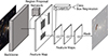 |
Fig. 2. Mask R-CNN architecture. Adapted from Jung et al. (2019). |
The Mask R-CNN architecture offers several key advantages over traditional CNNs when applied to lens detection tasks.
-
Instance segmentation. Unlike conventional CNNs that primarily perform image classification or basic object detection, Mask R-CNN generates detailed pixel-level segmentation masks for each detected object. It seamlessly integrates classification, bounding box regression, and segmentation tasks, whereas standard CNNs typically focus on a single task, such as whole-image classification.
-
Multi-object detection. Mask R-CNN is capable of detecting and segmenting multiple objects within a single image, even at different scales, while effectively distinguishing individual instances. In contrast, traditional CNNs often face challenges in identifying and separating overlapping objects.
-
Flexible input handling. Mask R-CNN can process images of varying sizes without the need to resize them to a fixed input dimension, unlike many standard CNN implementations. This flexibility helps preserve fine spatial details and prevents the loss of morphological information that can occur by interpolation during image resizing–an important advantage when working with high-resolution astrophysical data.
-
No need to produce the ‘negatives’. In the Mask R-CNN architecture every object that is not flagged as belonging to the ‘positive’ class (i.e. gravitational arcs) automatically pertains to the ‘negative’ one, removing in this way the need to create a fraction of the training set containing no arcs.
The code used in this work is based on the Python5 implementation of the Mask R-CNN from torchvision (TorchVision 2016), built on the pytorch framework (Paszke et al. 2019; Ansel et al. 2024). The initial stage of the Mask R-CNN utilises a pre-trained CNN, known as the ‘backbone’, to extract feature maps from input images. The standard Mask R-CNN model (He et al. 2017, maskrcnn_resnet50_fpn6 in torchvision) utilises as backbone the ResNet-50 residual NN (He et al. 2015). ResNets function as a feature extractor, with their initial layers capturing low-level features, such as edges and corners, and their deeper layers capturing high-level features via residual learning. ResNets are CNNs that employ ‘skip connections’, which allow the creation of deep architectures with many layers while avoiding the accuracy degradation issues commonly affecting deep NNs (He et al. 2015). This accuracy degradation happens because, as network depth increases, accuracy initially saturates and then swiftly declines (Bengio et al. 1994; He et al. 2017). The root cause of this problem lies in the backpropagation process, where continual multiplications by small weights diminish gradient sizes to the point of ineffectiveness; this issue is commonly known as the ‘vanishing gradient problem’ (Pascanu et al. 2012).
To handle objects of varying scales, features are extracted at different backbone stages and combined using a feature pyramid network (FPN; Lin et al. 2016), which integrates multiscale features by sharing information across hierarchical layers (Lakshmanan et al. 2021). The extracted feature maps are processed by the region proposal network (RPN; Ren et al. 2015), which generates object proposals using a sliding window approach that defines anchor boxes of varying sizes and aspect ratios at each spatial location on the feature map (Ren et al. 2015; Elgendy 2020). The RPN is trained to classify anchors as containing an object or not, while refining their bounding boxes, using a dedicated loss function to address both classification and regression tasks. In our implementation, we employ a set of anchors of sizes {32, 64, 128, 256, 512} pixels, with aspect ratios {0.5, 1, 2}. The subsampling factor of ResNet-50, i.e. the ratio by which the spatial dimensions of an image are reduced as it passes through the NN, is 32.
Non-maximum suppression (NMS; Girshick 2015) is subsequently applied to the proposed anchor boxes. This procedure begins by sorting all generated boxes according to their objectness scores, i.e. the confidence estimated by the network that a given region contains an object of interest. The algorithm then iteratively selects the box with the highest score and compares it against all remaining boxes using the intersection over union (IoU) metric,
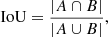 (2)
(2)
where A and B denote two bounding boxes, the numerator represents the area of their intersection, while the denominator corresponds to the area of their union. To filter the RPN proposals, we adopt the default threshold of IoU (He et al. 2017). Boxes that exhibit high IoU overlap with the selected box are suppressed, effectively removing redundant proposals. This process is repeated with the next highest-scoring unsuppressed box until all boxes have been processed or a predefined maximum number of proposals is reached. NMS thus helps reduce computational load and enhances detection accuracy by retaining only the most promising, non-overlapping candidate regions.
The highest-ranked boxes, determined by their likelihood of containing an ‘object’, are selected as the region of interest (RoI) for the following stage of the pipeline. In our work, we categorise RoIs into two classes, ‘gravitational arcs’ and ‘background’; the latter, being trivial, was not considered.
In the final stage of the Mask R-CNN, three tasks are performed simultaneously: a softmax classifier assigns probabilities for K + 1 categories (K = 1 in our case since we have only the ‘gravitational arcs’ class, while the +1 is for the background), a regression module refines bounding box coordinates, and a fully convolutional network generates pixel-wise binary masks within the RoI for semantic segmentation. The overall loss function of the Mask R-CNN is computed as the sum of these three contributions.
Transfer learning is a technique that enables NNs to leverage knowledge acquired from one task to enhance performance on a related but distinct task (refer to Tan et al. 2018 for an overview). This methodology capitalises on pre-existing weight values derived from one dataset, employing them as the foundation for network initialisation for training the network on another dataset. The advantages of this technique are twofold: it accelerates the training process, and it mitigates network overfitting.
In our work, we utilise as a starting point the Mask R-CNN weights pre-trained on the Microsoft Common Objects in Context (MS COCO; Lin et al. 2014) dataset. The MS COCO is a large-scale object detection, segmentation, key-point detection, and captioning dataset. It consists of 328 000 RGB 3-channel images of common objects, categorised into 91 classes. By utilizing transfer learning, we leverage the “universal” low-level geometric features learned from the images in MS COCO (e.g. edges, curves, and corners), allowing our model to generalise effectively despite the small number of instances in our training set. This allows the subsequent training on our specialised dataset to focus exclusively on learning the high-level morphology unique to gravitational arcs. After initialising the pre-trained NN parameters, we made trainable all its ≈44 million parameters, including also the backbone ones.
3.2. Data preparation
Since the pytorch implementation of Mask R-CNN is designed for standard 3-channel RGB images, an additional pre-processing step was required to retain as much information as possible. The third channel was then created by averaging the JE and HEEuclid bands (henceforth called the JHE band). The three RGB channels are thus JHE, YE, and IE, respectively.
Before feeding each image to the NN, we standardised the intensity of the pixels of each image. First, we clipped each band of the images independently at the 98th-percentile. Then, for each band of each image in the training set, we rescaled the pixel values using the z-score normalisation (Bishop & Bishop 2023), in order for the input image values to span a similar range of values, as
 (3)
(3)
 (4)
(4)
 (5)
(5)
where ⟨IE⟩ is the average value of the mean of the images in the IE-band, while σIE is the average standard deviation, both computed over the whole training set (and similarly for the YE- and JHE-bands). This allows for a faster convergence of the NN and prevents vanishing or exploding gradients (LeCun et al. 2012). This standardisation also ensures that the NN is not affected by the exposure time, detector gain, or the final normalisation of the pipeline-reduced images. The same data standardisation is then applied to real images during the inference phase.
We performed data augmentation on the training set, which makes the NN invariant with respect to the included transformations applied (Mikołajczyk & Grochowski 2018). In particular, we augmented the data by randomly applying to each image the following transformations, preserving classes, bounding boxes, and object masks:
-
horizontal flip, with 50% probability;
-
vertical flip, with 50% probability.
These basic augmentations replicate additional observational setups and conditions with minimal computational overhead, aiding the NN in better generalising its results.
3.3. Loss function
During training, each sampled RoI has a corresponding multitask loss representing the three assignments of the Mask R-CNN (classification, location, and segmentation), expressed as LRoI = Lcls + Lbox + Lmask (He et al. 2017). The classification loss is Lcls = −lnpu, where pu is the probability estimate from the NN for the true class u and a discrete probability distribution p = (p0, …, pK) is computed by a softmax on the output of a fully connected layer over K + 1 classes for each RoI (Girshick 2015). The bounding box loss Lbox again follows the definition in Girshick (2015), using an L1 smooth loss of the offsets between predicted and real bounding boxes for each of the K object classes. For the mask branch, which contains K binary masks of resolution m × m for each class (m being the size of the RoI), a per-pixel sigmoid function is applied, leading to Lmask being the average binary cross-entropy loss (refer to He et al. 2017 for the details). The final training loss L is the combination of the classification, box, and mask losses from the final branches of the Mask R-CNN along with the classification and box losses from the RPN (Lakshmanan et al. 2021).
3.4. Training
To train the NN, we used an improved version of the stochastic gradient descent algorithm (SGD; Goodfellow et al. 2016). SGD updates the model weights Θ by minimising the loss function L(Θ), as described by
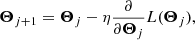 (6)
(6)
where η represents the learning rate, a hyperparameter that is fine-tuned to avoid local minima and ensure convergence.
In all epochs, we trained all the weights in all layers using a learning rate scheduler, starting with a value of η = 10−3 and gradually decreasing it by a factor of 0.5 every 20 epochs. This approach facilitates deeper learning and more precise tuning of the weights while at the same time reducing the risk of overfitting (Goodfellow et al. 2016). The SGD optimiser was initialised with a momentum value of 0.9, and a weight decay coefficient of 5 × 10⁻⁴. Furthermore, to prevent overfitting we included the early stopping regularisation (Prechelt 1997; Raskutti et al. 2011).
We trained the NN for 100 epochs in total, processing 4000 training and 500 validation 3 × 1199 × 1199 pixel images per epoch, in batches of 16. We used a single NVIDIA Quadro RTX 6000 GPU, with 3840 cores and 24 GB GDDR5 memory, to train on 4000 simulated 3-band FITS images. The training took approximately ten hours to complete (wall time). After this initial cost to train the NN, detection and inference on images of the same size can be performed in a fraction of a second.
4. Results
In this section, we present the results of the training, the performance of the NN, and the results of the application to real Euclid imaging data. We begin by testing the model’s performance using traditional ML metrics for classification tasks. Following this, we examine the outcomes of applying the trained Mask R-CNN to real Euclid Q1 observations, in order to assess its performance in discovering bright gravitational arcs in real galaxy cluster images.
4.1. Performance metrics
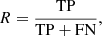
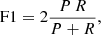
Two classes are present in our dataset, the gravitational arcs (‘positive’ class) and everything else, i.e. the background and all other astronomical objects (‘negative’ class). We use the MS COCO Evaluation Metrics (Lin et al. 2014) to quantitatively evaluate the performance of the NN. In particular, to measure the classification performance on the test dataset, we compute precision (or purity, P), recall (or completeness, R), and F1 score (their harmonic mean). Precision tells us how many of the positive predictions of the model are actually correct. Recall, on the other hand, is the ratio of correctly identified positive samples to the total number of actual positive samples in the dataset. These metrics are defined as
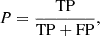 (7)
(7)
 (8)
(8)
 (9)
(9)
where TP stands for true positive, the number of objects correctly classified as the positive class; TN for true negative, the number of objects correctly classified as the negative class; FP for false positive, the number of objects incorrectly labelled as belonging to the positive class; and FN for false negative, the number of objects incorrectly labelled as belonging to the negative class.
A detection is considered ‘positive’ if its classification confidence score exceeds a specified minimum threshold pthr such that its predicted bounding box overlaps with the ground truth one, giving an IoU larger than a threshold (IoUthr). Therefore, TPs are identified when a detection has a confidence score above pthr and can be matched to a ground truth object with IoU > IoUthr; FNs refer to ground truth objects that lack a corresponding detection; and FPs are detections with a high confidence score that do not correspond to any ground truth object.
Precision and recall are not particularly informative when considered separately; an object detector is considered effective only if its precision remains high as recall increases (Ivezić et al. 2020). Therefore, to measure the performance of the NN, we use the average precision (AP) score (Everingham et al. 2010), a widely adopted metric in the DL and computer vision communities, which has superseded the area under the receiver operating characteristic curve. The AP (for a specific class) is calculated as the area under the precision-recall (P − R) curve, representing the precision averaged across uniformly distributed recall values from 0 to 1. Generally, a higher precision at a given recall value indicates superior model detection performance. This is evidenced by a larger area under the P − R curve; hence, higher AP values indicate better detection capabilities of the model. In this work, AP was computed for each image by averaging precision values at 101 equally spaced recall levels, R ∈ [0, 0.01, …, 1.0], namely as (Everingham et al. 2012)
![Mathematical equation: $$ \begin{aligned} \mathrm{AP} = \frac{1}{101} \sum _{R \in [0, 0.01, \ldots , 1.0]} P(R), \end{aligned} $$](/articles/aa/full_html/2026/07/aa57590-25/aa57590-25-eq20.gif) (10)
(10)
where P(R) is the maximum precision within the interval ΔR. We then calculate the average of the P − R curves and mean AP scores across all test set images.
In the MS COCO evaluation metrics, the network’s ability to distinguish and classify objects is assessed by computing AP in different ways. We use the standard AP score variants commonly used in the computer vision field. First, we repeat the computation of AP varying IoUthr from 0.50 to 0.95 in steps of 0.05, resulting in ten sets of P − R curves. The ten AP values derived from these ten sets are then averaged and denoted as AP@50 : 5 : 95, the primary COCO challenge metric. Then, AP50 (the Pascal VOC metric; Everingham et al. 2010) and AP75 are the AP metrics computed with IoUthr fixed at 0.5 and 0.75, respectively. Additionally, the AP for objects of different pixel areas is computed to evaluate the network’s detection performance across various object sizes. For gravitational arcs detection, objects with an area smaller than 162 pixels are denoted as APS, those with an area between 162 and 322 pixels are denoted as APM, and those larger than 322 pixels are denoted as APL, calculated using the same IoU threshold range as that of AP@50 : 5 : 957. The average recall (AR) instead is the maximum recall given a fixed number of detections per image (100 in our case), averaged over all the categories and IoU threshold values ranging from 0.50 to 0.95 in steps of 0.05.
4.2. Performance on the test set
In Fig. 3 we show the training history of the total loss and its individual components as a function of the training epoch for both training and validation sets. The validation loss value stabilised after approximately 20 iterations.
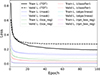 |
Fig. 3. Training history of the total loss and all its individual components as a function of the training epoch for the training (solid lines) and validation (dashed lines) datasets. The total loss (black lines) is the sum of the classification, box, and mask losses from the Mask R-CNN, along with the classification and box losses from the RPN. |
As an example of the inference, we show in Fig. 4 the result of the application of the trained Mask R-CNN on a galaxy cluster belonging to the test set, and thus, not seen during the training phase. The green bounding boxes correspond to the ground truth, i.e. they enclose the gravitational arcs present in the galaxy cluster (both the real and simulated ones), while the red dashed boxes are the final proposed ‘positives’ by the NN. We can see from this example that the NN correctly recovers all the largest gravitational arcs, missing only the smaller ones and producing a few false positives.
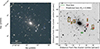 |
Fig. 4. Left: Euclidised 2′×2′ RGB image (R = JHE, G = YE, B = IE) of the galaxy cluster Abell 1063 belonging to the test set. The right-most arc is the one injected via SL simulation, while the others are real. Right: Single channel 2′×2′ Euclidised IE image of the same cluster. The green boxes enclose the gravitational arcs (both real and simulated) present in the field, i.e. the ground truth, while the red dashed boxes are the ‘gravitational arcs’ found by the NN, which have an object confidence score greater than 0.996. |
In Table 3, we present the COCO AP and AR metrics used to assess the performance of the NN on the test set, showing the model’s accuracy across various IoU thresholds and object sizes. These metrics offer insight into the strengths and limitations of the network. We observe that both AP and AR increase with arc size, with the best performance achieved in the large object category. This is expected, since larger arcs are more easily distinguishable from background structures and provide more pixels for the network to identify and segment. In contrast, smaller arcs are more affected by noise, and are often harder to resolve, given the resolution and depth of the images. This trend is also a direct consequence of the fact that our training set included only simulated arcs with an area larger than 400 pixels, biasing the network towards high completeness and purity in the detection of large arcs. Furthermore, the comparison between AP50 (54.3%) and AP75 (20.1%) highlights that while the NN is relatively good at localising arcs with moderate overlap, it struggles to precisely match their shape and boundaries – a known challenge in segmenting faint, irregular sources.
Summary of AP and AR bounding box results of the NN on the test set.
In Fig. 5a we present the three P − R curves for IoUthr = 0.5, 0.75, and @50:5:958, each obtained by varying the object score classification threshold pthr. In Fig. 5b we show the P − R curve for IoUthr = 0.5, where the dots are colour coded by the score threshold pthr used to evaluate them. Finally, in Fig. 5c we show the precision and the recall as a function of the score threshold for IoUthr = 0.5. By choosing a fixed value of the object probability threshold, pthr = 0.996, which can be tuned depending if we want to maximise precision over completeness, or vice versa, we can then compute the precision, recall, and F1 score of the NN on the test set, obtaining P = 75.9%, R = 58.0%, and F1 = 65.8%.
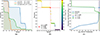 |
Fig. 5. Panel (a): Two sets of three P − R curves for IoUthr = 0.5, 0.75, @50:5:95, each obtained by varying the object score threshold pthr. Panel (b): P − R curve for IoUthr = 0.5, where the dots are colour-coded by the score threshold pthr used to evaluate them. In particular, we emphasise the P − R pair associated with our choice of score threshold pthr = 0.996. Note that the recall remains relatively high even at moderate precision, reflecting the network’s ability to recover most bright arcs while keeping the number of false positives manageable. Increasing the threshold shifts the operating point towards higher precision at the expense of recall. The extended horizontal segments are an artefact of the test set construction: all 500 test images are simulations based on the same cluster (Abell 1063). As a consequence, a subset of detections (and their associated confidence scores) remains identical across the test set, producing clustered score values and thus plateau-like features in the PR curve. Panel (c): Two precision and the recall curves as a function of the score threshold for IoUthr = 0.5. |
We note that the test set is composed of images containing several positive examples by construction. In a realistic scenario, where most clusters do not host giant arcs, the effective precision would decrease due to the lower prevalence of true positives relative to false positives.
4.3. Inference on Euclid Q1 lens clusters
As a further test, we wanted to assess the performance of the NN on the 20 galaxy clusters with lens probability 𝒫lens > 0.90 obtained from the Euclid Collaboration: Bergamini et al. (2026) visual inspection. They presented the first catalogue of SL galaxy clusters identified in the Euclid Q1 observations, based on a systematic visual inspection of 1260 richness-selected galaxy clusters from Wen & Han (2024), over an effective area of 4.4 deg2. They identified 83 gravitational lenses with 𝒫lens > 0.5, including 14 systems with 𝒫lens = 1 that exhibit secure SL features such as giant tangential and radial arcs, as well as multiple images.
In Fig. 6, we show in blue the distribution of the areas of the visually selected gravitational arcs9; in particular, we highlight the fact that the majority of them (≈65%) have an area which is smaller than the minimum area used in the training set for the simulated arcs (i.e. 400 pixels, indicated in the plot by the black dashed line). The red line instead shows the area distribution of the gravitational arcs correctly recovered by the NN. As expected, the majority of arcs with area larger than the training threshold are found (12/18 ≈ 66%). Overall, by considering all the arcs found during the visual inspection in the 20𝒫lens > 0.90 galaxy clusters as the ground truth for a further test set, the NN achieves a precision value of P = 19%, and recall of R = 42%. In Appendix A we show the predictions of the NN as bounding boxes over-plotted on the images of these 20 Euclid Q1 clusters, alongside the real arcs found during the visual inspection.
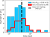 |
Fig. 6. Distribution of area in pixels of the gravitational arcs found by expert astronomers in the 20 Euclid Q1 clusters with 𝒫lens > 90% (Euclid Collaboration: Bergamini et al. 2026). The dashed red line shows the minimum value of the area of the arcs used as the ground truth for the training (400 pixels). |
5. Discussion
Despite the promising results, certain limitations remain. Bright stars and elongated shapes occasionally mimicking arcs, produce false positives, highlighting the need for improved pre-processing of the images and more diversity in the training set. Increasing the prevalence of such challenging objects in the training set could help the network better distinguish true arcs from lens-like false positives. While the simulated dataset effectively mimics real observations, the reliance on simulations may limit generalisability. As Euclid acquires more observational data, the performance of the Mask R-CNN is expected to improve for several reasons. With more real Euclid observations available, we can generate larger and more representative training datasets. This will help mitigate domain shift issues between simulated and real data, improving the generalisation of the network. Moreover, new mock datasets can be generated with more realistic arc properties, taking into account improved lens models, observational systematics, and the full range of image conditions and artefacts in Euclid data. For instance, using real Euclid cluster images as the background onto which mock lensed sources are injected ensures that the simulations accurately reflect the properties of the actual observations, including realistic noise, PSF, photometric depth, and the presence of instrumental features such as diffraction spikes or saturated stars. Once a sufficiently large real dataset is available, fine-tuning the existing Mask R-CNN model with actual Euclid images, rather than only relying on simulated arcs, will lead to better performance.
While the average precision and average recall test set results for large arcs (APL and ARL) are promising, the situation for medium- and small-sized ones reflected the inherent challenges in detecting these structures, which are often faint, blended with cluster galaxies, and affected by noise. In our work, we aimed particularly at detecting large bright gravitational arcs; therefore, the arcs injected in the training set reflected this goal. With continued improvements in training datasets, preprocessing, and model architecture, the detection of medium-sized arcs is expected to improve. However, small arcs will remain particularly challenging to detect due to their intrinsically low signal-to-noise ratios, and the higher abundance of small objects in the field that can mimic arc-like morphologies, compared to the rarer large arc-like features that are not genuine arcs.
6. Summary and conclusions
In this paper, we have developed a DL methodology to autonomously identify cluster-scale SL gravitational arcs within Euclid multi-band imaging of galaxy clusters. The challenges of gravitational arc detection in wide-field surveys are well-suited for the Mask R-CNN architecture, an advanced computer vision framework offering several important advantages over traditional CNNs. First, it performs instance segmentation, generating detailed pixel-level masks for each detected object by integrating classification, bounding box regression, and segmentation into a unified framework. Standard CNNs, instead, are typically limited to single-task operations such as whole-image classification. In addition, Mask R-CNN can detect and segment multiple objects within a single image, even when they appear at different scales or overlap, effectively distinguishing individual instances, something conventional CNNs often struggle with. Another important advantage is interpretability: The pixel-level segmentation masks produced by the Mask R-CNN framework makes it possible to visualise exactly which image regions the network has identified as arcs. This aids in understanding the origin of false positives, a task that is far more challenging with conventional CNNs that provide only image-level classifications. Finally, it can handle input images of varying sizes without requiring resizing to a fixed dimension, preserving structural details. In this context, our work represents one of the first applications of instance segmentation networks to the automated detection of cluster-scale gravitational arcs in real survey data, paving the way for future large-scale lensing searches in Euclid and other wide-field surveys.
The effectiveness of the network in detecting and classifying GCSLs within Euclid images is evaluated through several standard DL performance metrics. We also assess the capability of the NN to recover bright gravitational arcs in real Euclid Q1 observations, comparing the results of the inference with those obtained by human experts in a visual inspection (Euclid Collaboration: Bergamini et al. 2026). Our analysis on the test set revealed that the Mask R-CNN framework performs well in arc detection, achieving a good level of precision-recall trade-off. Notably, the architecture’s ability to simultaneously localise, classify, and segment arcs streamlined the detection process and facilitated accurate identification in crowded fields such as those of galaxy clusters. The successful application of this framework to real Euclid Q1 images has validated its practical utility, with the majority of large arcs identified aligning with expert classifications.
The Mask R-CNN framework was selected for this study due to its strong performance in instance segmentation and its ability to simultaneously classify, localise, and segment gravitational arcs. It is not necessarily the definitive or optimal solution, and there are several alternative architectures that could be explored in future work to further improve arc detection and segmentation, including U-Nets (Ronneberger et al. 2015) and YOLOs (Redmon et al. 2016); such networks, however, generally perform poorer on typical computer vision benchmarks (He et al. 2017).
Deploying the NN blindly across all Euclid tiles would inevitably lead to a significant number of false positives, which, while expected, would require extensive post-processing. The best strategy would be then to apply the network primarily to a selected subset of the richest galaxy clusters rather than across the entire survey tiles. This approach aims to balance minimising false positives with ensuring that genuine SL events are not missed. Moreover, while the DL models provide a fairly high level of accuracy in arc detection, a human validation step remains crucial to minimise false positives and ensure high purity in the final candidate sample. This step can be performed by expert astronomers visually inspecting the top-ranked candidates. A key advantage of our approach lies in its ability to significantly reduce the visual inspection effort required in large-scale surveys. In the Euclid Collaboration: Bergamini et al. (2026) analysis of Euclid Q1 data, around 40 experts visually examined approximately 1300 candidate clusters, selected with a cut on richness from the Wen & Han (2024) catalogue. This process, while effective, is not scalable to future releases; indeed, Euclid Collaboration: Bergamini et al. (2026) estimate that, with the same number of human experts, it would take more than 15 years to visually inspect the entire EWS area.
This study further illustrates the potential of DL techniques in astrophysics, enabling the efficient and automated analysis of gravitational lensing phenomena in large-scale surveys. As current and next-generation surveys will produce unprecedentedly large datasets, advanced computer vision methodologies such as this will be crucial in unlocking the full potential of these observations.
Acknowledgments
We thank the anonymous referee for the helpful and insightful comments that improved the paper. We acknowledge financial support through grant 2020SKSTHZ. LB is indebted to the communities behind the multiple free, libre, and open-source software packages on which we all depend. MM was supported by INAF Grants “The Big-Data era of cluster lensing” and “Probing Dark Matter and Galaxy Formation in Galaxy Clusters through Strong Gravitational Lensing”, and ASI Grant n. 2024-10-HH.0 “Attività scientifiche per la missione Euclid – fase E”. The research activities described in this paper have been co-funded by the European Union – NextGeneration EU within PRIN 2022 project no. 20229YBSAN – Globular clusters in cosmological simulations and in lensed fields: from their birth to the present epoch. The Euclid Consortium acknowledges the European Space Agency and a number of agencies and institutes that have supported the development of Euclid, in particular the Agenzia Spaziale Italiana, the Austrian Forschungsförderungsgesellschaft funded through BMIMI, the Belgian Science Policy, the Canadian Euclid Consortium, the Deutsches Zentrum für Luft- und Raumfahrt, the DTU Space and the Niels Bohr Institute in Denmark, the French Centre National d’Etudes Spatiales, the Fundação para a Ciência e a Tecnologia, the Hungarian Academy of Sciences, the Ministerio de Ciencia, Innovación y Universidades, the National Aeronautics and Space Administration, the National Astronomical Observatory of Japan, the Netherlandse Onderzoekschool Voor Astronomie, the Norwegian Space Agency, the Research Council of Finland, the Romanian Space Agency, the State Secretariat for Education, Research, and Innovation (SERI) at the Swiss Space Office (SSO), and the United Kingdom Space Agency. A complete and detailed list is available on the Euclid website (www.euclid-ec.org). This work has made use of the Euclid Quick Release Q1 data from the Euclid mission of the European Space Agency (ESA), 2025, https://doi.org/10.57780/esa-2853f3b. This work used the following software packages: Python (Van Rossum & Drake 2009), PyTorch (Paszke et al. 2019; Ansel et al. 2024), torchvision (TorchVision 2016), NumPy (van der Walt et al. 2011; Harris et al. 2020), SciPy (Virtanen et al. 2020), scikit-learn (Pedregosa et al. 2011), Astropy (Astropy Collaboration 2013, 2018), matplotlib (Hunter 2007), LENSTOOL (Kneib et al. 1996; Jullo et al. 2007; Jullo & Kneib 2009), ds9 (Joye & Mandel 2003), Aladin (Bonnarel et al. 2000), topcat (Taylor 2005), git, bash (GNU 2007).
References
- Acebron, A., Cibirka, N., Zitrin, A., et al. 2018, ApJ, 858, 42 [NASA ADS] [CrossRef] [Google Scholar]
- Acevedo Barroso, J. A., O’Riordan, C. M., Clément, B., et al. 2025, A&A, 697, A14 [Google Scholar]
- Angora, G., Rosati, P., Brescia, M., et al. 2020, A&A, 643, A177 [NASA ADS] [CrossRef] [EDP Sciences] [Google Scholar]
- Angora, G., Rosati, P., Meneghetti, M., et al. 2023, A&A, 676, A40 [NASA ADS] [CrossRef] [EDP Sciences] [Google Scholar]
- Ansel, J., Yang, E., & He, H. 2024, 29th ACM International Conference on Architectural Support for Programming Languages and Operating Systems, Volume 2 (ASPLOS ’24) (ACM) [Google Scholar]
- Astropy Collaboration (Robitaille, T. P., et al.) 2013, A&A, 558, A33 [NASA ADS] [CrossRef] [EDP Sciences] [Google Scholar]
- Astropy Collaboration (Price-Whelan, A. M., et al.) 2018, AJ, 156, 123 [Google Scholar]
- Auger, M. W., Treu, T., Gavazzi, R., et al. 2010, ApJ, 721, L163 [Google Scholar]
- Bailer-Jones, C. A. L., Fouesneau, M., & Andrae, R. 2019, MNRAS, 490, 5615 [CrossRef] [Google Scholar]
- Bazzanini, L., Ferro, L., Guidorzi, C., et al. 2024, A&A, 689, A266 [NASA ADS] [CrossRef] [EDP Sciences] [Google Scholar]
- Bengio, Y., Simard, P., & Frasconi, P. 1994, IEEE Trans. Neural Networks, 5, 157 [Google Scholar]
- Bergamini, P., Rosati, P., Mercurio, A., et al. 2019, A&A, 631, A130 [NASA ADS] [CrossRef] [EDP Sciences] [Google Scholar]
- Bergamini, P., Rosati, P., Vanzella, E., et al. 2021, A&A, 645, A140 [EDP Sciences] [Google Scholar]
- Bergamini, P., Acebron, A., Grillo, C., et al. 2023a, A&A, 670, A60 [NASA ADS] [CrossRef] [EDP Sciences] [Google Scholar]
- Bergamini, P., Acebron, A., Grillo, C., et al. 2023b, ApJ, 952, 84 [NASA ADS] [CrossRef] [Google Scholar]
- Bishop, C., & Bishop, H. 2023, Deep Learning: Foundations and Concepts (Springer International Publishing) [Google Scholar]
- Bonamigo, M., Grillo, C., Ettori, S., et al. 2017, ApJ, 842, 132 [NASA ADS] [CrossRef] [Google Scholar]
- Bonamigo, M., Grillo, C., Ettori, S., et al. 2018, ApJ, 864, 98 [Google Scholar]
- Bonnarel, F., Fernique, P., Bienaymé, O., et al. 2000, A&AS, 143, 33 [NASA ADS] [CrossRef] [EDP Sciences] [Google Scholar]
- Burke, C. J., Aleo, P. D., Chen, Y.-C., et al. 2019, MNRAS, 490, 3952 [NASA ADS] [CrossRef] [Google Scholar]
- Caminha, G. B., Grillo, C., Rosati, P., et al. 2017, A&A, 607, A93 [NASA ADS] [CrossRef] [EDP Sciences] [Google Scholar]
- Caminha, G. B., Rosati, P., Grillo, C., et al. 2019, A&A, 632, A36 [NASA ADS] [CrossRef] [EDP Sciences] [Google Scholar]
- Caminha, G. B., Suyu, S. H., Grillo, C., & Rosati, P. 2022, A&A, 657, A83 [NASA ADS] [CrossRef] [EDP Sciences] [Google Scholar]
- Cañameras, R., Schuldt, S., Suyu, S., et al. 2020, A&A, 644, A163 [NASA ADS] [CrossRef] [EDP Sciences] [Google Scholar]
- Cao, S., Covone, G., & Zhu, Z.-H. 2012, ApJ, 755, 31 [NASA ADS] [CrossRef] [Google Scholar]
- Capak, P., Aussel, H., Ajiki, M., et al. 2007, ApJS, 172, 99 [Google Scholar]
- Clarke, A. O., Scaife, A. M. M., Greenhalgh, R., & Griguta, V. 2020, A&A, 639, A84 [NASA ADS] [CrossRef] [EDP Sciences] [Google Scholar]
- Collett, T. E. 2015, ApJ, 811, 20 [NASA ADS] [CrossRef] [Google Scholar]
- Collett, T. E., & Auger, M. W. 2014, MNRAS, 443, 969 [NASA ADS] [CrossRef] [Google Scholar]
- D’Isanto, A., & Polsterer, K. L. 2018, A&A, 609, A111 [Google Scholar]
- Elgendy, M. 2020, Deep Learning for Vision Systems (Manning) [Google Scholar]
- Elíasdóttir, Á., Limousin, M., Richard, J., et al. 2007, ArXiv e-prints [arXiv:0710.5636] [Google Scholar]
- Euclid Collaboration (Adam, R., et al.) 2019, A&A, 627, A23 [NASA ADS] [CrossRef] [EDP Sciences] [Google Scholar]
- Euclid Collaboration (Scaramella, R., et al.) 2022, A&A, 662, A112 [NASA ADS] [CrossRef] [EDP Sciences] [Google Scholar]
- Euclid Collaboration (Leuzzi, L., et al.) 2024, A&A, 681, A68 [NASA ADS] [CrossRef] [EDP Sciences] [Google Scholar]
- Euclid Collaboration (Bergamini, P., et al.) 2025, A&A, 702, A73 [Google Scholar]
- Euclid Collaboration (Cropper, M., et al.) 2025, A&A, 697, A2 [Google Scholar]
- Euclid Collaboration (Jahnke, K., et al.) 2025, A&A, 697, A3 [Google Scholar]
- Euclid Collaboration (Mellier, Y., et al.) 2025, A&A, 697, A1 [Google Scholar]
- Euclid Collaboration (Aussel, H., et al.) 2026, A&A, 711, A1 [Google Scholar]
- Euclid Collaboration (Bergamini, P., et al.) 2026, A&A, 711, A33 [Google Scholar]
- Euclid Collaboration (Walmsley, M., et al.) 2026, A&A, 711, A26 [Google Scholar]
- Euclid Quick Release Q1 2025, https://doi.org/10.57780/esa-2853f3b [Google Scholar]
- Everingham, M., Van Gool, L., Williams, C. K., Winn, J., & Zisserman, A. 2010, Int. J. Comput. Vision, 88, 303 [CrossRef] [Google Scholar]
- Everingham, M., Van Gool, L., Williams, C. K. I., Winn, J., & Zisserman, A. 2012, The PASCAL Visual Object Classes Challenge 2012 (VOC2012) Results, http://www.pascal-network.org/challenges/VOC/voc2012/workshop/index.html [Google Scholar]
- Farias, H., Ortiz, D., Damke, G., Jaque Arancibia, M., & Solar, M. 2020, Astron. Comput., 33, 100420 [NASA ADS] [CrossRef] [Google Scholar]
- Gavazzi, R., Marshall, P. J., Treu, T., & Sonnenfeld, A. 2014, ApJ, 785, 144 [Google Scholar]
- Girshick, R. 2015, ArXiv e-prints [arXiv:1504.08083] [Google Scholar]
- GNU, P. 2007, Free Software Foundation. Bash (3.2. 48)[Unix shell program] [Google Scholar]
- Goodfellow, I., Bengio, Y., & Courville, A. 2016, Deep Learning (MIT Press), http://www.deeplearningbook.org [Google Scholar]
- Green, J., Schechter, P., Baltay, C., et al. 2012, ArXiv e-prints [arXiv:1208.4012] [Google Scholar]
- Grillo, C., Rosati, P., Suyu, S. H., et al. 2018, ApJ, 860, 94 [Google Scholar]
- Grillo, C., Pagano, L., Rosati, P., & Suyu, S. H. 2024, A&A, 684, L23 [NASA ADS] [CrossRef] [EDP Sciences] [Google Scholar]
- Harris, C. R., Millman, K. J., van der Walt, S. J., et al. 2020, Nature, 585, 357 [NASA ADS] [CrossRef] [Google Scholar]
- He, K., Zhang, X., Ren, S., & Sun, J. 2015, ArXiv e-prints [arXiv:1512.03385] [Google Scholar]
- He, K., Gkioxari, G., Dollár, P., & Girshick, R. 2017, ArXiv e-prints [arXiv:1703.06870] [Google Scholar]
- He, Y., Wu, J., Wang, W., Jiang, B., & Zhang, Y. 2023, PASJ, 75, 1311 [NASA ADS] [CrossRef] [Google Scholar]
- Huang, X., Storfer, C., Ravi, V., et al. 2020, ApJ, 894, 78 [NASA ADS] [CrossRef] [Google Scholar]
- Huertas-Company, M., & Lanusse, F. 2023, PASA, 40, e001 [NASA ADS] [CrossRef] [Google Scholar]
- Hunter, J. D. 2007, Comput. Sci. Eng., 9, 90 [NASA ADS] [CrossRef] [Google Scholar]
- Ivezić, Ž., Kahn, S. M., Tyson, J. A., et al. 2019, ApJ, 873, 111 [Google Scholar]
- Ivezić, Ž., Connolly, A., VanderPlas, J., & Gray, A. 2020, Statistics, Data Mining, and Machine Learning in Astronomy: A Practical Python Guide for the Analysis of Survey Data, Updated Edition, Princeton Series in Modern Observational Astronomy (Princeton University Press) [Google Scholar]
- Jackson, N. 2008, MNRAS, 389, 1311 [NASA ADS] [CrossRef] [Google Scholar]
- Jia, P., Sun, R., Li, N., et al. 2023, AJ, 165, 26 [NASA ADS] [CrossRef] [Google Scholar]
- Joye, W. A., & Mandel, E. 2003, ASP Conf. Ser., 295, 489 [Google Scholar]
- Jullo, E., & Kneib, J. P. 2009, MNRAS, 395, 1319 [NASA ADS] [CrossRef] [Google Scholar]
- Jullo, E., Kneib, J. P., Limousin, M., et al. 2007, New J. Phys., 9, 447 [Google Scholar]
- Jullo, E., Natarajan, P., Kneib, J. P., et al. 2010, Science, 329, 924 [Google Scholar]
- Jung, H., Lodhi, B., & Kang, J. 2019, BMC Biomed. Eng., 1, 1 [Google Scholar]
- Keeton, C. R. 2001, ArXiv e-prints [arXiv:astro-ph/0102340] [Google Scholar]
- Kinney, A. L., Calzetti, D., Bohlin, R. C., et al. 1996, ApJ, 467, 38 [NASA ADS] [CrossRef] [Google Scholar]
- Kneib, J. P., Ellis, R. S., Smail, I., Couch, W. J., & Sharples, R. M. 1996, ApJ, 471, 643 [Google Scholar]
- Lagattuta, D. J., Richard, J., Bauer, F. E., et al. 2019, MNRAS, 485, 3738 [NASA ADS] [Google Scholar]
- Lagattuta, D. J., Richard, J., Bauer, F. E., et al. 2022, MNRAS, 514, 497 [NASA ADS] [CrossRef] [Google Scholar]
- Laigle, C., McCracken, H. J., Ilbert, O., et al. 2016, ApJS, 224, 24 [Google Scholar]
- Lakshmanan, V., Görner, M., & Gillard, R. 2021, Practical Machine Learning for Computer Vision (O’Reilly Media) [Google Scholar]
- Lao, B., Jaiswal, S., Zhao, Z., et al. 2023, Astron. Comput., 44, 100728 [Google Scholar]
- Le Fèvre, O., & Hammer, F. 1988, ApJ, 333, L37 [CrossRef] [Google Scholar]
- LeCun, Y., Bottou, L., Bengio, Y., & Haffner, P. 1998, Proc. IEEE, 86, 2278 [Google Scholar]
- LeCun, Y. A., Bottou, L., Orr, G. B., & Müller, K.-R. 2012, Efficient BackProp (Berlin, Heidelberg: Springer), 9 [Google Scholar]
- LeCun, Y., Bengio, Y., & Hinton, G. 2015, Nature, 521, 436 [Google Scholar]
- Limousin, M., Kneib, J.-P., & Natarajan, P. 2005, MNRAS, 356, 309 [Google Scholar]
- Lin, T. Y., Maire, M., Belongie, S., et al. 2014, ArXiv e-prints [arXiv:1405.0312] [Google Scholar]
- Lin, T. Y., Dollár, P., Girshick, R., et al. 2016, ArXiv e-prints [arXiv:1612.03144] [Google Scholar]
- Lombardi, M., & Bertin, G. 1999, A&A, 342, 337 [NASA ADS] [Google Scholar]
- Lombardi, M., Rosati, P., Blakeslee, J. P., et al. 2005, ApJ, 623, 42 [NASA ADS] [CrossRef] [Google Scholar]
- Lotz, J., Mountain, M., Grogin, N. A., et al. 2014, Am. Astron. Soc. Meet. Abstr., 223, 254.01 [NASA ADS] [Google Scholar]
- Lotz, J. M., Koekemoer, A., Coe, D., et al. 2017, ApJ, 837, 97 [Google Scholar]
- Marshall, P. J., Verma, A., More, A., et al. 2016, MNRAS, 455, 1171 [NASA ADS] [CrossRef] [Google Scholar]
- Meneghetti, M. 2021, Introduction to Gravitational Lensing: With Python Examples, Lecture Notes in Physics (Springer International Publishing) [Google Scholar]
- Meneghetti, M., Melchior, P., Grazian, A., et al. 2008, A&A, 482, 403 [NASA ADS] [CrossRef] [EDP Sciences] [Google Scholar]
- Meneghetti, M., Fedeli, C., Pace, F., Gottlöber, S., & Yepes, G. 2010, A&A, 519, A90 [NASA ADS] [CrossRef] [EDP Sciences] [Google Scholar]
- Meneghetti, M., Ragagnin, A., Borgani, S., et al. 2022, A&A, 668, A188 [NASA ADS] [CrossRef] [EDP Sciences] [Google Scholar]
- Merz, G., Liu, Y., Burke, C., et al. 2024, Am. Astron. Soc. Meet. Abstr., 243, 302.03 [Google Scholar]
- Metcalf, R. B., & Petkova, M. 2014, MNRAS, 445, 1942 [NASA ADS] [CrossRef] [Google Scholar]
- Metcalf, R. B., Meneghetti, M., Avestruz, C., et al. 2019, A&A, 625, A119 [NASA ADS] [CrossRef] [EDP Sciences] [Google Scholar]
- Metcalfe, N., Shanks, T., Campos, A., McCracken, H. J., & Fong, R. 2001, MNRAS, 323, 795 [Google Scholar]
- Mikołajczyk, A., & Grochowski, M. 2018, 2018 International Interdisciplinary PhD Workshop (IIPhDW), 117 [Google Scholar]
- Millon, M., Galan, A., Courbin, F., et al. 2020, A&A, 639, A101 [NASA ADS] [CrossRef] [EDP Sciences] [Google Scholar]
- More, A., Cabanac, R., More, S., et al. 2012, ApJ, 749, 38 [NASA ADS] [CrossRef] [Google Scholar]
- Moresco, M., Amati, L., Amendola, L., et al. 2022, Liv. Rev. Relat., 25, 6 [NASA ADS] [Google Scholar]
- Mueed Hafiz, A., & Mohiuddin Bhat, G. 2020, Int J Multimed Info Retr, 9, 171 [Google Scholar]
- Oke, J. B., & Gunn, J. E. 1983, ApJ, 266, 713 [NASA ADS] [CrossRef] [Google Scholar]
- Pascanu, R., Mikolov, T., & Bengio, Y. 2012, ArXiv e-prints [arXiv:1211.5063] [Google Scholar]
- Paszke, A., Gross, S., Massa, F., et al. 2019, ArXiv e-prints [arXiv:1912.01703] [Google Scholar]
- Pawase, R. S., Courbin, F., Faure, C., Kokotanekova, R., & Meylan, G. 2014, MNRAS, 439, 3392 [NASA ADS] [CrossRef] [Google Scholar]
- Pedregosa, F., Varoquaux, G., Gramfort, A., et al. 2011, J. Mach. Learn. Res., 12, 2825 [Google Scholar]
- Pence, W. D., Chiappetti, L., Page, C. G., Shaw, R. A., & Stobie, E. 2010, A&A, 524, A42 [NASA ADS] [CrossRef] [EDP Sciences] [Google Scholar]
- Petkova, M., Metcalf, R. B., & Giocoli, C. 2014, MNRAS, 445, 1954 [NASA ADS] [CrossRef] [Google Scholar]
- Petrillo, C. E., Tortora, C., Chatterjee, S., et al. 2017, MNRAS, 472, 1129 [Google Scholar]
- Postman, M., Coe, D., Benítez, N., et al. 2012, ApJS, 199, 25 [Google Scholar]
- Prechelt, L. 1997, Neural Networks: Tricks of the Trade, Volume 1524 of LNCS, Chapter 2 (Springer-Verlag), 55 [Google Scholar]
- Raskutti, G., Wainwright, M. J., & Yu, B. 2011, 2011 49th Annual Allerton Conference on Communication, Control, and Computing (Allerton), 1318 [Google Scholar]
- Redmon, J., Divvala, S., Girshick, R., & Farhadi, A. 2016, Proceedings of the IEEE Conference on Computer Vision and Pattern Recognition, 779 [Google Scholar]
- Ren, S., He, K., Girshick, R., & Sun, J. 2015, ArXiv e-prints [arXiv:1506.01497] [Google Scholar]
- Richard, J., Kneib, J.-P., Ebeling, H., et al. 2011, MNRAS, 414, L31 [Google Scholar]
- Ronneberger, O., Fischer, P., & Brox, T. 2015, Medical Image Computing and Computer-assisted Intervention–MICCAI 2015: 18th International Conference, Munich, Germany, October 5–9, 2015, Proceedings, Part III 18, Springer, 234 [Google Scholar]
- Schuldt, S., Suyu, S. H., Cañameras, R., et al. 2021, A&A, 651, A55 [NASA ADS] [CrossRef] [EDP Sciences] [Google Scholar]
- Scoville, N., Aussel, H., Brusa, M., et al. 2007, ApJS, 172, 1 [Google Scholar]
- Seidel, G., & Bartelmann, M. 2007, A&A, 472, 341 [NASA ADS] [CrossRef] [EDP Sciences] [Google Scholar]
- Sérsic, J. L. 1963, Boletin de la Asociacion Argentina de Astronomia La Plata Argentina, 6, 41 [Google Scholar]
- Sérsic, J. L. 1968, Atlas de Galaxias Australes (Cordoba, Argentina: Observatorio Astronomico) [Google Scholar]
- Shibuya, T., Ouchi, M., & Harikane, Y. 2015, ApJS, 219, 15 [Google Scholar]
- Sonnenfeld, A., Treu, T., Gavazzi, R., et al. 2013, ApJ, 777, 98 [Google Scholar]
- Sonnenfeld, A., Treu, T., Marshall, P. J., et al. 2015, ApJ, 800, 94 [Google Scholar]
- Sonnenfeld, A., Chan, J. H. H., Shu, Y., et al. 2018, PASJ, 70, S29 [Google Scholar]
- Sonnenfeld, A., Verma, A., More, A., et al. 2020, A&A, 642, A148 [NASA ADS] [CrossRef] [EDP Sciences] [Google Scholar]
- Suyu, S. H., Bonvin, V., Courbin, F., et al. 2017, MNRAS, 468, 2590 [Google Scholar]
- Swinbank, A. M., Webb, T. M., Richard, J., et al. 2009, MNRAS, 400, 1121 [NASA ADS] [CrossRef] [Google Scholar]
- Sygnet, J. F., Tu, H., Fort, B., & Gavazzi, R. 2010, A&A, 517, A25 [NASA ADS] [CrossRef] [EDP Sciences] [Google Scholar]
- Tan, C., Sun, F., Kong, T., et al. 2018, ArXiv e-prints [arXiv:1808.01974] [Google Scholar]
- Tanoglidis, D., Ćiprijanović, A., Drlica-Wagner, A., et al. 2022, Astron. Comput., 39, 100580 [NASA ADS] [CrossRef] [Google Scholar]
- Taylor, M. B. 2005, ASP Conf. Ser., 347, 29 [Google Scholar]
- TDCOSMO Collaboration (Birrer, S., et al.) 2025, A&A, 704, A63 [Google Scholar]
- TorchVision 2016, TorchVision: PyTorch’s Computer Vision Library, https://github.com/pytorch/vision [Google Scholar]
- Tortora, C., Napolitano, N. R., Romanowsky, A. J., & Jetzer, P. 2010, ApJ, 721, L1 [NASA ADS] [CrossRef] [Google Scholar]
- Tortorelli, L., Mercurio, A., Paolillo, M., et al. 2018, MNRAS, 477, 648 [NASA ADS] [CrossRef] [Google Scholar]
- Treu, T., & Koopmans, L. V. E. 2002, ApJ, 575, 87 [NASA ADS] [CrossRef] [Google Scholar]
- van der Walt, S., Colbert, S. C., & Varoquaux, G. 2011, Comput. Sci. Eng., 13, 22 [Google Scholar]
- Van Rossum, G., & Drake, F. L. 2009, Python 3 Reference Manual (Scotts Valley: CreateSpace) [Google Scholar]
- Vanzella, E., Meneghetti, M., Caminha, G. B., et al. 2020, MNRAS, 494, L81 [Google Scholar]
- Vanzella, E., Caminha, G. B., Rosati, P., et al. 2021, A&A, 646, A57 [EDP Sciences] [Google Scholar]
- Virtanen, P., Gommers, R., Oliphant, T. E., et al. 2020, Nat. Meth., 17, 261 [Google Scholar]
- Wen, Z. L., & Han, J. L. 2024, ApJS, 272, 39 [NASA ADS] [CrossRef] [Google Scholar]
- Williams, R. E., Blacker, B., Dickinson, M., et al. 1996, AJ, 112, 1335 [NASA ADS] [CrossRef] [Google Scholar]
- Xu, B., Postman, M., Meneghetti, M., et al. 2016, ApJ, 817, 85 [Google Scholar]
- Yang, Y., Li, X., Bai, X., et al. 2019, ApJ, 887, 129 [NASA ADS] [CrossRef] [Google Scholar]
- Yang, P., Bai, H., Zhao, L., et al. 2023, A&A, 677, A121 [NASA ADS] [CrossRef] [EDP Sciences] [Google Scholar]
These lens models are publicly available at https://www.fe.infn.it/astro/lensing/
Notice that the values of APS, APM, and APL used in our work are smaller with respect to those in the COCO Evaluation Metrics, since the pixel areas of gravitational arcs are generally smaller than typical COCO images.
@50:5:95 means the value of the reference metric obtained by averaging it over IoU thresholds of IoUthr ∈ {0.50, 0.55, …, 0.95}.
These binary masks were manually drawn based on the bounding boxes surrounding the lensing events provided by the expert astronomers in Euclid Collaboration: Bergamini et al. (2026).
Appendix A: Predictions on Euclid Q1 clusters
In this Appendix, we show the inference results of the trained Mask R-CNN on the 20𝒫lens > 0.90 galaxy clusters from Euclid Collaboration: Bergamini et al. (2026). The NN has been applied on a 2′×2′ MER cutout on the nominal centre of the cluster, according to the catalogue. The red masks enclose the real arcs identified by expert astronomers; the dashed rectangles instead show the predicted ‘gravitational arcs’ by the NN, using the object score threshold pthr = 0.996 employed for the test set (cf. Fig. 4). We note the presence of false positives, often associated with bright elongated galaxies, edge-on discs, or image artefacts that mimic arc-like morphologies, highlighting the need for further refinement of the training data or post-processing steps.
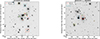 |
Fig. A.1. VIS cutouts with size 2′×2′ of the 20𝒫lens > 0.90 galaxy clusters from Euclid Collaboration: Bergamini et al. (2026). The red masks enclose the real arcs identified by expert astronomers; the dashed rectangles show the predictions of the NN. |
All Tables
All Figures
|
Fig. 1. Steps of a Euclid GCSL simulation. Left: HST2EUCLID 2′×2′ RGB image of the galaxy cluster Abell S1063 (zcl = 0.348), with the main critical line (in red) for a source at zs = 2.92, based on the lens model by Bergamini et al. (2019). The critical line has a circularised Einstein radius of θE ≃ 33″. The green cross marks the position of the injected source to be lensed. Middle: Source plane at zs = 2.92 displaying the caustic (in red) related to the main critical line. The injected source (green cross) features a Sérsic profile (index n = 1.22, |
| In the text | |
|
Fig. 2. Mask R-CNN architecture. Adapted from Jung et al. (2019). |
| In the text | |
|
Fig. 3. Training history of the total loss and all its individual components as a function of the training epoch for the training (solid lines) and validation (dashed lines) datasets. The total loss (black lines) is the sum of the classification, box, and mask losses from the Mask R-CNN, along with the classification and box losses from the RPN. |
| In the text | |
|
Fig. 4. Left: Euclidised 2′×2′ RGB image (R = JHE, G = YE, B = IE) of the galaxy cluster Abell 1063 belonging to the test set. The right-most arc is the one injected via SL simulation, while the others are real. Right: Single channel 2′×2′ Euclidised IE image of the same cluster. The green boxes enclose the gravitational arcs (both real and simulated) present in the field, i.e. the ground truth, while the red dashed boxes are the ‘gravitational arcs’ found by the NN, which have an object confidence score greater than 0.996. |
| In the text | |
|
Fig. 5. Panel (a): Two sets of three P − R curves for IoUthr = 0.5, 0.75, @50:5:95, each obtained by varying the object score threshold pthr. Panel (b): P − R curve for IoUthr = 0.5, where the dots are colour-coded by the score threshold pthr used to evaluate them. In particular, we emphasise the P − R pair associated with our choice of score threshold pthr = 0.996. Note that the recall remains relatively high even at moderate precision, reflecting the network’s ability to recover most bright arcs while keeping the number of false positives manageable. Increasing the threshold shifts the operating point towards higher precision at the expense of recall. The extended horizontal segments are an artefact of the test set construction: all 500 test images are simulations based on the same cluster (Abell 1063). As a consequence, a subset of detections (and their associated confidence scores) remains identical across the test set, producing clustered score values and thus plateau-like features in the PR curve. Panel (c): Two precision and the recall curves as a function of the score threshold for IoUthr = 0.5. |
| In the text | |
|
Fig. 6. Distribution of area in pixels of the gravitational arcs found by expert astronomers in the 20 Euclid Q1 clusters with 𝒫lens > 90% (Euclid Collaboration: Bergamini et al. 2026). The dashed red line shows the minimum value of the area of the arcs used as the ground truth for the training (400 pixels). |
| In the text | |
|
Fig. A.1. VIS cutouts with size 2′×2′ of the 20𝒫lens > 0.90 galaxy clusters from Euclid Collaboration: Bergamini et al. (2026). The red masks enclose the real arcs identified by expert astronomers; the dashed rectangles show the predictions of the NN. |
| In the text | |
Current usage metrics show cumulative count of Article Views (full-text article views including HTML views, PDF and ePub downloads, according to the available data) and Abstracts Views on Vision4Press platform.
Data correspond to usage on the plateform after 2015. The current usage metrics is available 48-96 hours after online publication and is updated daily on week days.
Initial download of the metrics may take a while.