


| Issue |
A&A
Volume 710, June 2026
|
|
|---|---|---|
| Article Number | A401 | |
| Number of page(s) | 17 | |
| Section | Extragalactic astronomy | |
| DOI | https://doi.org/10.1051/0004-6361/202660207 | |
| Published online | 01 July 2026 | |
H I absorption in MHONGOOSE
Spin temperatures and cold neutral medium in nearby disc galaxies
1
Netherlands Institute for Radio Astronomy (ASTRON), Oude Hoogeveensedijk 4, 7991 PD, Dwingeloo, The Netherlands
2
Department of Astronomy, University of Cape Town, Private Bag X3 Rondebosch 7701, South Africa
3
Kapteyn Astronomical Institute, University of Groningen, PO Box 800, 9700 AV, Groningen, The Netherlands
4
INAF – Osservatorio Astronomico di Cagliari, Via della Scienza 5, I-09047 Selargius, (CA), Italy
5
Wits Centre for Astrophysics, School of Physics, University of the Witwatersrand, 1 Jan Smuts Avenue, 2000 Johannesburg, South Africa
6
Université de Strasbourg, CNRS, Observatoire astronomique de Strasbourg, UMR 7550, 67000 Strasbourg, France
7
INAF – Arcetri Astrophysical Observatory, Largo Enrico Fermi 5, 50125 Firenze, Italy
8
Dipartimento di Fisica e Astronomia, Università degli Studi di Firenze, Via G. Sansone 1, 50019 Sesto Fiorentino, Firenze, Italy
9
Max Planck Institute for Radio Astronomy, Auf dem Hügel 69, 53121 Bonn, Germany
10
National Centre for Radio Astrophysics, Tata Institute of Fundamental Research, Pune University Campus, Post Bag 3, Ganeshkhind, Pune 411007, India
11
Jodrell Bank Centre for Astrophysics, School of Physics and Astronomy, University of Manchester, Oxford Road, Manchester M13 9PL, UK
★ Corresponding author: This email address is being protected from spambots. You need JavaScript enabled to view it.
Received:
2
April
2026
Accepted:
10
May
2026
Abstract
Combined H I emission–absorption studies constrain the spin temperature and phase structure of the neutral atomic hydrogen interstellar medium (ISM). However, these studies have largely been limited to the Milky Way and the Local Group. We extend this technique to galaxies at distances of 7–22 Mpc using deep data from the MeerKAT H I Observations of Nearby Galactic Objects – Observing Southern Emitters (MHONGOOSE) survey and quantify the detection fraction and cold neutral medium (CNM) properties at these distances. We searched for H I absorption towards 56 background continuum sources in 21 out of the 30 MHONGOOSE galaxies (with nine galaxies lacking suitable background sources) and detected absorption associated with the H I discs of the galaxies in three cases: one sightline in NGC 289 and two in NGC 7424. This corresponds to detection rates of 5% (3/56) for the full sample and 10% (3/31) for a clean sub-sample of sightlines when considering only unresolved background sources behind 14 low-inclination galaxies. Detections occur only where both the continuum flux and the foreground H I column density are high, with optical-depth sensitivity as the primary limiting factor. For the detected sightlines, we modelled the absorption and emission spectra to derive spin temperatures and CNM fractions using the standard combined emission–absorption method. The CNM spin temperatures and line widths are comparable to Local Group measurements, but the inferred CNM fractions are systematically lower. We argue that this difference is primarily a resolution effect. At the distances of our galaxies, the emission spectra average over several hundred parsecs, diluting structured CNM relative to the smoother warm neutral medium. This demonstrates that emission–absorption analyses can be extended beyond the Local Group, provided that care is taken in constructing representative emission spectra.
Key words: ISM: structure / galaxies: ISM / galaxies: spiral / galaxies: structure / radio lines: ISM
© The Authors 2026
 Open Access article, published by EDP Sciences, under the terms of the Creative Commons Attribution License (https://creativecommons.org/licenses/by/4.0), which permits unrestricted use, distribution, and reproduction in any medium, provided the original work is properly cited.
This article is published in open access under the Subscribe to Open model. This email address is being protected from spambots. You need JavaScript enabled to view it. to support open access publication.
1. Introduction
Neutral atomic hydrogen (H I) is the dominant baryonic component of the interstellar medium (ISM) in most disc galaxies, and it provides the reservoir from which molecular gas and stars form. Observations of the H I 21-cm radio line play an important role in studies of galaxy structure, kinematics, and evolution.
The atomic ISM can be described in terms of two phases in approximate pressure equilibrium (Field et al. 1969; Wolfire et al. 1995, 2003; McClure-Griffiths et al. 2023). The cold neutral medium (CNM) has characteristic temperatures of ∼10 K to ∼100 K, while the warm neutral medium (WNM) has temperatures of ∼104 K. Quantifying how atomic gas is distributed between these phases and how this distribution varies with galaxy properties or environment remains a key goal in ISM studies. The CNM has a lower volume-filling factor and represents the atomic phase most directly connected to molecular clouds and star formation. The WNM is more diffuse, dominates the volume, and traces the larger-scale distribution of the ISM.
The spin temperature (Ts) is the excitation temperature that describes the relative population of the two hyperfine levels of the ground state of the neutral hydrogen atom, and it provides a direct constraint on the physical state of the H I. The spin temperature is set by a competition between collisional coupling, Lyα scattering, and the ambient radiation field. In the CNM, the high densities ensure that collisions dominate, so the spin temperature approximates the kinetic temperature. In the WNM, the collision process is inefficient due to the lower densities, and Ts is instead determined by a combination of Lyα coupling and the background radiation field, resulting in values of a few times 103 K that are generally lower than the kinetic temperature (Liszt 2001).
Most studies of galaxies in H I are based on 21-cm emission, which is produced by both the WNM and CNM. Emission by itself provides only limited information on the phase structure of the ISM. For example, cold gas can become optically thick, affecting the proportionality between measured emission and column density, narrow CNM emission components can blend with more dominant and broader WNM components along the line of sight, and emission measurements can be affected by beam dilution when the angular scale of H I structures is smaller than the telescope beam. Since the CNM is often organised into compact structures, this can bias emission-based estimates of its properties.
H I absorption offers a complementary constraint. Due to the higher absorption efficiency of cold gas set by the hyperfine level populations of H I and the inverse dependence of the optical depth on spin temperature, absorption against a background radio continuum source primarily traces the cold component of the foreground gas, i.e. the CNM. When absorption and emission measurements are combined, in principle, constraining the CNM contribution to the emission spectrum becomes possible. One complication is that absorption measurements probe a narrow pencil-beam line of sight, while emission measurements are averaged over the telescope resolution and usually taken at positions adjacent to the absorber. The underlying assumption that both types of measurements trace the same structures may not always be valid, and this becomes increasingly critical at larger distances.
The most detailed combined emission–absorption measurements can be carried out in the Milky Way (MW), owing to both the large number of bright background continuum sources and the high physical resolution of the observations. H I surveys (e.g. Dickey & Lockman 1990; Heiles & Troland 2003a,b; Dickey et al. 2003; Murray et al. 2015, 2018, 2021; McClure-Griffiths et al. 2023) have shown that emission and absorption spectra often differ substantially and that these differences can be explained by the coexistence of cold and warm gas along the line of sight. These studies show that the CNM constitutes a significant fraction of the Galactic H I, with a broad distribution of spin temperatures and a preference for values between ∼40 K and ∼70 K. Kanekar et al. (2011) used absorption measurements in the MW to identify a rapid change in spin temperature at a column density of ∼2 × 1020 cm−2, interpreted as the threshold for CNM formation.
The Magellanic Clouds (MCs) are the closest environment outside the MW where the phases of the ISM can be studied under different physical conditions, including lower metallicity and stronger radiation fields. The MCs generally have a lower CNM fraction compared to the MW (e.g. Stanimirovic et al. 1999; Dickey et al. 2000; Jameson et al. 2019; Dempsey et al. 2022). Absorption detections in M31 and M33 have been used to measure the properties of cold atomic gas in other Local Group galaxies (e.g. Dickey & Brinks 1988, 1993; Braun & Walterbos 1992). Pingel et al. (2024) reported absorption detections in the Local Group dwarf galaxy NGC 6822 and derived spin temperatures and CNM fractions.
Outside the Local Group (at distances beyond ∼1 Mpc), background continuum sources such as active galactic nuclei (AGNs) or quasars are not only used as probes but can themselves be the targets of absorption studies. In many cases, the absorption arises in the AGN itself rather than in an intervening galaxy. This associated absorption probes the circumnuclear environment. Central regions of AGNs typically do not show cold gas in H I emission. However, about 30% of them show cold gas absorption, allowing the cold components to be traced (Maccagni et al. 2017). In many cases, this absorption traces inflows and outflows interpreted as jet–ISM interaction (Morganti & Oosterloo 2018).
In the case of intervening absorption, the absorbing gas is unrelated to the emitting source and instead probes neutral gas in galaxy discs and halos along the line of sight between the observer and the background emitter. Many studies of intervening absorption have been guided by searches for damped Lyman-α (DLA) and Mg II absorbers, which in many cases have defined the samples for 21-cm absorption follow-up (e.g. Lane 2000; Kanekar & Chengalur 2003; Kanekar et al. 2009). It is not clear to what extent this pre-selection introduces biases in, for example, metallicity or dust content.
Wide-field H I absorption surveys conducted with Square Kilometre Array (SKA) pathfinder and precursor telescopes should help mitigate these biases by avoiding selection based on optical absorption. Two of these surveys are the MeerKAT Absorption Line Survey (MALS; Gupta et al. 2016) and the First Large Absorption Survey in H I (FLASH; Allison et al. 2022). The first, MALS, is a deep unbiased search for H I and OH absorption over the redshift range 0 < z < 2, and it targets both intervening absorbers and absorption associated with radio-loud AGNs. The aim of the second survey, FLASH, is to detect several hundred intervening and associated absorbers over 0.4 < z < 1.0 towards bright radio continuum sources using wide-field observations.
These surveys provide a census of cold atomic gas at intermediate redshifts that are difficult to access via H I emission. Detailed, spatially resolved studies of nearby systems with absorption can help interpret, among other things, the observed detection rates, the distribution of impact parameters, the phase balance of the ISM, and any dependence on galaxy type.
Absorption-based constraints on the CNM and WNM in the local Universe outside the Local Group remain limited to a small number of systems and sightlines. For example, early observations of galaxy-quasar pairs are presented by Carilli & van Gorkom (1992), with additional examples of intervening absorption in nearby galaxies reported by Borthakur et al. (2014), Dutta et al. (2016), Gupta et al. (2018). Maina et al. (2022) detected absorption in the Klemola 31 group at z = 0.029, associated with the H I disc of a group member. In a study of 16 nearby gas-rich galaxies comprising 24 sightlines, Reeves et al. (2015, 2016) detected absorption along one line of sight. Many of these studies are limited by angular resolution, complicating the comparison between absorption and emission spectra.
In this work we used data from the MeerKAT H I Observations of Nearby Galactic Objects: Observing Southern Emitters (MHONGOOSE) survey1 (de Blok et al. 2024) to study the intervening absorption in nearby galaxies. MHONGOOSE provides deep, high-resolution H I observations of disc and dwarf galaxies, probing one to two orders of magnitude deeper in column density than previous surveys. We analysed spectra along sightlines towards these galaxies to quantify the detection fraction and the properties of the detected absorption. By applying the combined emission–absorption analysis traditionally used in Local Group studies, we derived spin temperatures and CNM fractions for galaxies at distances of 7–22 Mpc, i.e. an order of magnitude more distant than those probed in previous work.
In Sect. 2 we briefly describe the MHONGOOSE H I data and the additional processing required to produce the absorption data. In Sect. 3 we review the necessary background on combined emission–absorption studies and introduce the equations and methodology used in the remainder of the paper. Section 4 presents the selection of the continuum sample and the corresponding spectra. In Sect. 5 we discuss the absorption detections and derive their physical properties. In Sect. 6 we examine the possible reasons for the non-detections, and Sect. 7 provides a summary of the paper.
2. MHONGOOSE
The MHONGOOSE survey (de Blok et al. 2024) is a deep H I survey of 30 nearby (D < 23 Mpc) disc and dwarf galaxies. Its main science goals are to study the accretion processes by which galaxies obtain sufficient gas to sustain star formation, and the relation between this gas and star formation in these systems. MHONGOOSE is the deepest interferometric H I survey to date, with each galaxy observed for 55 h with MeerKAT, reaching a column density sensitivity of ∼5 × 1017 cm−2 (3σ over 16 km s−1) at a resolution of ∼1′–1.5′. For a full description of the survey parameters and data reduction procedures, see de Blok et al. (2024).
To cover the full resolution range available with MeerKAT, MHONGOOSE H I data products were created at six ‘standard’ resolutions, spanning ∼7″ to ∼90″, using different combinations of robust weighting and tapering. The highest-resolution maps are created using a robust value of zero without tapering (r00_t00), yielding angular resolutions of ∼7″. At this resolution, the noise in a single 1.4 km s−1 channel is 0.22 mJy beam−1, corresponding to a column density sensitivity of ∼6 × 1019 cm−2 (3σ over 16 km s−1).
The continuum measurement sets of the MHONGOOSE galaxies are created during the self-calibration procedure that forms part of the standard reduction pipeline (see de Blok et al. 2024 for details). They cover the frequency range 1390–1420 MHz. Initial imaging revealed direction-dependent artefacts in some fields, necessitating additional direction-dependent calibration, for which we used the oxkat (Heywood 2020) package. The final continuum images were created by combining the ten direction-dependent-calibrated measurement sets for each galaxy and imaging them using a robust weighting parameter of zero and without tapering (i.e. identical to the r00_t00 H I data). We used the masks created by the oxkat package for the deconvolution. The noise level in these continuum images is ∼3.3 μJy beam−1.
3. Combining absorption and emission spectra
As the methodology of deriving and combining absorption and emission spectra plays a key role in interpreting our data and in defining the sample of background continuum sources, we briefly review the key equations and procedures here. Further details can be found in, for example, Dickey et al. (1992, 2003), Heiles & Troland (2003a,b), Murray et al. (2021), McClure-Griffiths et al. (2023) and Pingel et al. (2024).
The basic radiative transfer equation is
 (1)
(1)
where TB(v) is the brightness temperature at velocity v, Ts is the spin temperature of the gas, and τ(v) is the optical depth. For optically thin gas (τ ≪ 1), we can approximate this as
 (2)
(2)
When H I is observed in absorption against a background continuum source with flux density Scont, the observed flux density as a function of velocity reflects the effect of foreground gas on the background continuum. This can be written as
![Mathematical equation: $$ \begin{aligned} S(v) = S_{\rm cont} [(1 - c_f) + c_f e^{-\tau (v)}]. \end{aligned} $$](/articles/aa/full_html/2026/06/aa60207-26/aa60207-26-eq3.gif) (3)
(3)
Here cf is the covering factor of the absorbing gas. Defining the absorption depth as ΔS(v) = Scont − S(v), we can rewrite this as
 (4)
(4)
In the optically thin limit, this becomes
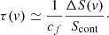 (5)
(5)
The H I column density is related to the optical-depth profile through
 (6)
(6)
This expression shows that once the optical depth spectrum τ(v) has been determined, the inferred column density scales linearly with the assumed spin temperature Ts and inversely with the covering factor cf. The latter is not always known, and often cf = 1 is assumed.
In the optically thin limit, the H I column density is related to the brightness temperature spectrum TB(v) through Eqs. (2) and (6). It can be written as
 (7)
(7)
This expression is independent of optical depth and shows that optically thin gas can contribute substantially to the observed emission while producing only weak absorption. This difference underlies the fundamental distinction between absorption and emission. Absorption traces the CNM through τ(v), whereas emission traces the combined contribution of both CNM and WNM through TB(v).
We modelled the absorption and emission spectra as combinations of Gaussian components. Since the CNM produces measurable absorption, we parameterise it directly through its optical-depth profile, τ(v). The corresponding CNM emission TB(v) can then be derived from τ(v) and the radiative transfer equation (Eq. (1)).
For the absorption spectrum, which in practice traces the CNM-dominated absorbing gas, the optical depth can be written as the sum of N Gaussian components so that
![Mathematical equation: $$ \begin{aligned} \tau (v) = \sum _{n=0}^{N-1} \tau _{0,n} \exp [-(v - v_{0,n})^2/(2\sigma _{v,n}^2)]. \end{aligned} $$](/articles/aa/full_html/2026/06/aa60207-26/aa60207-26-eq8.gif) (8)
(8)
Each Gaussian represents a different CNM cloud or component, characterised by its peak optical depth τ0, n, central velocity v0, n, and velocity dispersion σv, n. The full widths at half maximum (FWHM) are given by  .
.
The emission spectrum, in contrast, contains contributions from both the CNM and the WNM. We write its expected brightness temperature as
 (9)
(9)
For the CNM, the emission follows directly from Eq. (1). In contrast, the WNM has low optical depth and does not typically produce detectable absorption (but see Killerby-Smith et al. 2025; Patra et al. 2018). It must therefore be constrained from the emission spectrum alone. We modelled the WNM directly in brightness temperature space, describing its contribution as a sum of K Gaussian components,
![Mathematical equation: $$ \begin{aligned} T_{B,\mathrm{WNM}}(v) = \sum _{k=0}^{K-1} T_{0,k} \exp [-(v - v_{0,k})^2/(2\sigma _{v,k}^2)]. \end{aligned} $$](/articles/aa/full_html/2026/06/aa60207-26/aa60207-26-eq11.gif) (10)
(10)
These WNM spectra must be modified to account for absorption by CNM components present between us and the WNM components along the line of sight. For the case of a single CNM component, we introduce a factor Fk that describes the fraction of WNM emission lying in front of the absorbing CNM along the line of sight. This yields
![Mathematical equation: $$ \begin{aligned} T_{B,\mathrm{WNM}}(v) = \sum _{k=0}^{K-1} [ F_k + (1 - F_k)e^{-\tau (v)}]\, T_{0,k} \exp \left[-\frac{(v - v_{0,k})^2}{2\sigma _{v,k}^2}\right]. \end{aligned} $$](/articles/aa/full_html/2026/06/aa60207-26/aa60207-26-eq12.gif) (11)
(11)
In general, Fk is not used as a fit parameter. Instead we assume a number of values Fk = 0, 0.5, and 1 to cover the possible geometries. These correspond to the WNM lying entirely behind the CNM (maximum absorption), partially mixed with the CNM (intermediate absorption), or entirely in front of the CNM (no absorption), respectively.
When more than one CNM component is present, the radiative transfer becomes more complex, as each component emits its own radiation while also absorbing radiation from components located behind it along the line of sight. The total expected spectrum can be written as
![Mathematical equation: $$ \begin{aligned} \begin{aligned} T_{\rm exp}(v)&= \sum _{n=0}^{N-1} T_{s,n}(1-e^{-\tau _n(v)}) \exp \!\left[-\sum _{m < n}\tau _m(v)\right] \\&\quad + \sum _{k=0}^{K-1} \left[ F_k + (1-F_k)\exp \left(-\sum _{n=0}^{N-1}\tau _n(v)\right) \right] T_{0,k} \\&\quad \times \exp \left[-\frac{(v-v_{0,k})^2}{2\sigma _{v,k}^2}\right]. \end{aligned} \end{aligned} $$](/articles/aa/full_html/2026/06/aa60207-26/aa60207-26-eq13.gif) (12)
(12)
The observed emission spectrum alone does not uniquely determine the relative ordering of CNM and WNM components along the line of sight, as multiple arrangements can produce similar spectra. To address this degeneracy, we explored all permutations of the CNM-WNM geometry. For a single CNM component and K WNM components, this results in 3K distinct configurations, corresponding to the three possible values of Fk. In the general case of N CNM components, the number of possible permutations scales as N! 3K, reflecting both the ordering of the CNM clouds along the line of sight and the placement of the WNM components relative to them. Usually, the number of distinct solutions is somewhat smaller, as permutations involving nearly identical components produce spectra that are observationally indistinguishable.
In practice, the optical-depth spectrum, derived from the absorption spectrum, is first fitted to determine the number of CNM components N. This fixes the CNM optical-depth parameters τ0, n, the central velocities v0, n, and the velocity widths of the individual components σv, n. The observed emission spectrum is then fitted to determine the number of WNM components K, where the CNM optical-depth profiles τn(v) are treated as fixed parameters, and the CNM enters the emission modelling only through the spin temperatures Ts, n, which are free parameters.
Even with N and K fixed, an ambiguity remains in the relative line-of-sight arrangement of the CNM and WNM components, as encoded in the parameters Fk. Following the terminology of Heiles & Troland (2003a), each distinct combination of Fk values for fixed N and K defines a ‘trial’. Each trial is fitted to the observed emission spectrum. Because the data do not generally uniquely determine the true CNM-WNM geometry, no single trial can be preferred a priori. Instead, physical parameters are derived by averaging over all acceptable trials, that is, over all possible (combinations of) choices of Fk for fixed N and K. In particular, the final spin temperature Ts is computed as a weighted average over all trials (for a given N and K), with weights determined by the goodness of fit, following Eqs. (21a) and (21b) of Heiles & Troland (2003a).
From the fitted components, several additional physical diagnostics are computed. The maximum kinetic temperature of each component is given by Tk, max = mH/(8kBln2) ΔvFWHM2 = 21.866 ΔvFWHM2, providing an upper limit on the true kinetic temperature in the absence of non-thermal broadening. This is useful because in a CNM–WNM mixture the spin temperature generally differs from the kinetic temperature.
The CNM and WNM column densities are given by Eq. (6) and Eq. (7), respectively (with cf = 1). From these, the CNM fraction is defined as
 (13)
(13)
which quantifies the relative contribution of cold gas to the total neutral hydrogen column density.
Finally, we computed the density-weighted mean spin temperature (Dickey et al. 2000),
![Mathematical equation: $$ \begin{aligned} \langle T_s \rangle = \frac{\int T_B(v)\,dv}{\int [1 - e^{-\tau (v)}]\,dv}\cdot \end{aligned} $$](/articles/aa/full_html/2026/06/aa60207-26/aa60207-26-eq15.gif) (14)
(14)
This quantity provides a single effective temperature that reflects the relative importance of absorption and emission, with the denominator dominated by contributions from gas with significant optical depth (primarily the CNM) and the numerator incorporating emission from both CNM and WNM. We can understand this as follows: starting from Eq. (1), we get Ts(v) = TB(v)/[1 − e−τ(v)], but this quantity is poorly defined when τ(v) is small (as will be the case for the WNM). Instead, we can define a single effective temperature ⟨Ts⟩ that relates the velocity-integrated brightness temperatures and optical depth: ∫TB(v) dv = ⟨Ts⟩∫[1 − e−τ(v)] dv, resulting in the above expression for ⟨Ts⟩.
Finally, we emphasise an important limitation of combined emission–absorption analyses. Absorption probes a narrow line of sight towards a compact background source, whereas the corresponding emission spectrum is obtained from nearby positions and averaged over the larger telescope beam. This difference in spatial sampling becomes increasingly important at larger distances, where the physical scale of the beam grows and variations in the H I distribution and kinematics become more significant. The resulting mismatch introduces a systematic uncertainty that must be accounted for in the modelling and interpretation.
4. Results
4.1. Continuum source selection
In searching for absorption in the MHONGOOSE galaxies, we adopted a lower peak flux limit of Scont = 0.7 mJy beam−1 for the continuum sources considered. This threshold is set by the achievable optical-depth sensitivity of the data. For small optical depths, the 1σ uncertainty in optical depth is given by στ = σI/Scont, where σI is the per-channel rms noise. For the r00_t00 data, σI = 0.22 mJy beam−1. For Scont = 0.7 mJy beam−1, this yields a 1σ optical-depth sensitivity of στ ≃ 0.3.
Requiring a 3σ detection in optical depth implies sensitivity to peak optical depths of τ0 ∼ 0.9. At this limit, we are sensitive to absorption features with peak optical depths of order unity per channel. Sources fainter than 0.7 mJy beam−1 would only allow the detection of absorption with a very high optical depth. We excluded such sources from further consideration.
We used the Python Blob Detection and Source Finder (pybdsf; Mohan & Rafferty 2015) to identify all continuum sources in the primary-beam-corrected continuum images with peak flux densities > 0.7 mJy beam−1 that are spatially coincident with the H I discs, as defined by the r00_t00 zeroth-moment maps. These maps have an average 3σ column density sensitivity of 6 × 1019 cm−2. The 0.7 mJy beam−1 peak flux represents a signal-to-noise of ∼200 in the continuum images, so the source detection is unambiguous.
In the centres of galaxies NGC 1566 (J0419–54) and NGC 1672 (J0445–59), we detected absorption lines with widths of ∼60 − 100 km s−1 associated with the AGNs in these galaxies. We do not study these here, and excluded these central sources from the catalogue. The final list contains 56 continuum sources distributed over 21 galaxies. Nine MHONGOOSE galaxies were not included, as their H I distributions do not overlap with any sufficiently bright continuum sources.
4.2. Detections and non-detections
We extracted spectra from the r00_t00 data cubes at the positions of the continuum sources and detect absorption towards three of them. One detection is found in NGC 289 (J0052–31), towards NVSS J005245–311503 (NRAO VLA Sky Survey; Condon et al. 1998). Two additional detections in close proximity are found in NGC 7424 (J2257–41), towards SUMSS J225729–410241 (Sydney University Molonglo Sky Survey; Mauch et al. 2003) and the supernova SN2001ig. These spectra are shown in Fig. 1. We discuss them in more detail in Sect. 5. The properties of the three continuum sources are listed in Table 1.
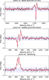 |
Fig. 1. Spectra of the three absorption profiles. From top to bottom: NVSS J005245−311503 in NGC 289 (J0052−31), SUMSS J225729−410241 in NGC 7424 (J2257−41), and SN2001ig also in NGC 7424 (J2257−41). The original spectra are shown in black, with a five-point Hanning-smoothed version overplotted in red. The 0, ±1σ, and ±2σ levels of the unsmoothed spectrum are indicated by solid, dashed, and dotted lines, respectively. |
Continuum sources with peak fluxes > 4 mJy overlapping the H I discs.
The remaining 53 spectra show no obvious evidence of absorption. We quantified this by using a simple detection criterion in which the spectra are smoothed with a five-point Hanning filter. For a detection, absorption is required to extend over more than two original channel widths below −3σ in the smoothed spectrum, and to be located within the velocity range of the galaxy as measured from the first-moment maps. A five-point Hanning smoothing changes the effective spectral resolution to approximately twice the original channel width, and the requirement that absorption extends over more than two original channels ensures that we are sensitive to features broader than a single smoothed resolution element.
To illustrate, we list the properties of the brightest non-detection background sources in Table 1 and show the corresponding spectra in Fig. A.1. The difference between the three detections and the non-detections is clear. All detections are highly significant, with peak S/N values > 10, and no detections are found at lower peak S/N.
To quantify the presence or absence of absorption as a function of the strength of the background continuum source and of the foreground H I emission, we measure the H I emission column density values in the r00_t00 zeroth-moment maps at the positions of the non-detection continuum sources. For the sources with absorption, we measure the column density in a one-beam-wide annulus with inner radius one beam, centred on the continuum position. We plot these column densities against the peak flux of the continuum sources in Fig. 2. We detect H I absorption only where both the continuum peak flux and the emission column density are high. The three absorption spectra all occur at emission column densities ∼1 × 1021 cm−2. Note the difference between the two strongest continuum sources. The ∼40 mJy beam−1 source SUMSS J225729–410241 shows absorption with a ∼1021 cm−2 foreground column density. The stronger (∼60 mJy beam−1) source SUMSS J030941–410006 has a foreground column density only a factor of ∼3 lower, yet shows no absorption. Sources fainter than 9 mJy beam−1 show no absorption regardless of column density.
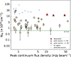 |
Fig. 2. H I emission column densities at the positions of the continuum sources plotted against continuum peak flux. The column densities are not corrected for inclination. Red triangles indicate detections. Circles indicate non-detections towards unresolved non-Hα sources, with filled symbols for i < 70° and open symbols for i ≥ 70°. Small stars indicate Hα star-forming regions, and small circles indicate resolved sources not associated with Hα. Filled circles mark the ‘clean’ sample of unresolved non-Hα sources in low-inclination galaxies. The horizontal dashed line shows the 3σ over 16 km s−1 column density limit of log(NH I/cm−2) = 19.77. |
The lack of absorption despite high column densities could, in some cases, be caused by projection effects along the line of sight due to high inclination values. This can allow a lower column density H I (primarily WNM) to accumulate along the line of sight, mimicking a high column density without a significant CNM component. In Fig. 2 we indicate all i > 70° galaxies with a different symbol, where inclinations are taken from de Blok et al. (2024). Of the 18 galaxies with low-Speak and high-NHI sight-lines, eight have a high inclination, but ten do not. For the latter, projection effects cannot cause the high column densities.
A fraction of the continuum sources turns out to be (somewhat) extended. This can reduce the probability of detecting absorption, as the effective covering factor cf may be less than unity. We identified sources with major axis size > 1.1 bmax or minor axis size > 1.1 bmin, where bmax and bmin are the major and minor axis of the beam, respectively. Comparison with Hα imaging from the Survey for Ionization in Neutral Gas Galaxies (Meurer et al. 2006) shows that most of these are associated with star-forming regions in the target galaxies. Of the 56 sources, 44 are unresolved (three with Hα) and 12 resolved (nine with Hα). Selecting unresolved non-Hα sources behind galaxies with i < 70° yields 31 sources in 14 galaxies. The different source types are indicated in Fig. 2. The ‘clean’ sample contains no sources with both low Speak and high NHI sightlines. We return to this in Sect. 6.1.
5. Absorption spectra
Here we present and analyse the three absorption spectra in more detail. We discuss the properties of the foreground galaxies, derive the intrinsic absorption-only spectra and discuss the additional difficulties of deriving and interpreting the emission spectra in objects at these distances. We present the properties of the CNM and WNM components along these three lines of sight.
5.1. Absorption in NGC 289
5.1.1. Properties of the galaxy and continuum source
We detected a single absorption line of sight in NGC 289 (J0052–31). This galaxy is among the most massive galaxies in the MHONGOOSE sample. It hosts a bright inner disc with a stellar bar and a faint outer low-surface-brightness disc containing several star-forming spiral arms. NGC 289 hosts a low-luminosity AGN, and is usually classified as a Seyfert galaxy. The galaxy is gas-rich, with its H I mass (2.2 × 10¹⁰ M⊙) almost equal to its stellar mass (2.7 × 10¹⁰ M⊙). We assumed a distance of 21.5 Mpc (Leroy et al. 2019), corresponding to 1″ = 0.1 kpc. NGC 289 is not part of any major group or cluster, but it resides in a low-density environment. Kourkchi & Tully (2017) list it as the main galaxy in its own sparse low-density association.
NGC 289 was studied in H I before by Walsh et al. (1997) using the Australia Telescope Compact Array (ATCA). In addition to the properties listed above, they also note the flat and extended rotation curve (with a maximum radius of over 50 kpc, adjusted to our assumed distance), the dark matter dominance of the low-surface brightness disc and the significant recent star formation in the far outer disc.
Inspection of the r00_t00 H I zeroth-moment map already reveals the presence of the absorption feature in the outer H I disc as shown in Fig. 3. It is also visible in the r05_t00 data (with an angular resolution of 11″), but not in the r10_t00 data (resolution 22″) or at lower resolutions, where the larger beam and increased emission filling dilute the absorption feature.
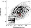 |
Fig. 3. Zeroth-moment map of NGC 289 based on the r00_t00 data. The red box in the main panel (1.6′×1.6′) marks the position of the absorption feature. The bottom-left inset shows a zoom-in of this region. The red ellipse indicates the continuum source. The r00_t00 beam is shown in the lower right. |
A Gaussian fit to the source in the continuum image shows it is unresolved. The flux listed for this source in NVSS at 1.4 GHz is 20.4 ± 1.1 mJy, consistent with the MHONGOOSE value listed in Table 1. NVSS J005245–311503 has an alternative identification (WISEA J005245.58–311503.2), and is visible in WISE bands W1 (3.4 μm) and W2 (4.6 μm). It is not visible in W3 and W4 (12 and 22 μm), respectively. In the Legacy Survey (Dey et al. 2019) we also find a faint optical counterpart at the position of the infrared source. Its colour is much redder than the surrounding disc emission of NGC 289, indicating it is likely a background source seen through the galactic disc. The projected galactocentric distance (impact parameter) of this detection is ∼17.5 kpc.
5.1.2. The absorption spectrum
Both the WNM and the CNM can cause absorption, though Eqs. (6) and (7) indicate that any absorption signal will be dominated by that of CNM absorption. Detections of WNM absorption in the MW exist, but they require extremely sensitive observations (see, e.g. Killerby-Smith et al. 2025 and Patra et al. 2018). Certainly, at the sensitivities of our observations, we expect the absorption signal to be fully dominated by the CNM.
Emission profiles, in contrast, contain of a more equal mix of CNM and WNM contributions. For a pure absorption measurement it is important to image the CNM absorption in isolation and avoid any contamination from the CNM and WNM emission. We created cubes containing only the absorption. As the absorption is due to a point source, while the emission is extended, this can be achieved by suppressing the signal on the short baselines (e.g. Dickey et al. 2003). We found that a robust value of −1 combined with removing (flagging) all baselines with a length below 1000 m, gives a good compromise between removing the H I emission and not amplifying the noise significantly. As we are interested in the absorption with respect to the continuum background, the absorption cube was created using measurement sets where the continuum was not subtracted. The beam size of this cube is 5.27″ × 5.10″ with 1″ pixels.
Due to the removal of the short baselines and the low robustness factor, the noise in the cube increases by about a factor of two to 0.41 mJy beam−1. This loss of sensitivity is also why these cubes are not used for source and absorption detection ab initio. To measure the intrinsic CNM absorption spectrum, we consider only pixels within the FWHM of the synthesised beam centred on the background continuum source. For each of these pixels, we measure the continuum flux density Scont from line-free channels in the velocity range 1300–1600 km s−1. Following Dickey et al. (1992), we then construct an averaged absorption spectrum from these pixel spectra. For each pixel, we use the spectrum S(v) from data without continuum subtraction and form the normalised spectrum S(v)/Scont, corresponding to e−τ(v) for cf = 1 (Eq. (4)). These normalised spectra are combined using weights proportional to the square of the continuum flux density in each pixel. This weighting emphasises high signal-to-noise pixels while preserving the intrinsic absorption profile. The resulting weighted average yields the intrinsic absorption spectrum in units of e−τ(v). The final spectrum is shown in Fig. 4.
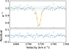 |
Fig. 4. Top: Intrinsic absorption spectrum of NVSS J005245−311503 in NGC 289 derived from the absorption-only data cube, shown as optical depth τ. The dashed line indicates zero optical depth, and the dotted lines indicate the ±1σ levels. A single-component Gaussian fit is overplotted. Bottom: Residuals with respect to the Gaussian fit. |
5.1.3. The emission spectrum
Absorption samples a pencil-beam line of sight towards a background continuum source. The corresponding emission spectrum, however, cannot be measured at that exact position and is therefore derived from nearby regions using a larger beam. Any combined absorption–emission analysis must assume that properties of the ISM at the absorption and emission positions are comparable. This assumption can often be justified for MW studies where the physical resolution can reach sub-parsec scales.
The situation quickly becomes more complicated with increasing distance. Chen et al. (2025) note in their study of the LMC and the SMC that with a spatial resolution of ∼8 pc, an offset of a beam or two may already lead to emission spectra that are not tracing exactly the same regions as the absorption spectrum, and contain different emission components.
In many previous studies the emission spectrum is derived by interpolating across the absorber position (e.g. Dickey et al. 1992), or by averaging the spectra in a region around the absorber. For example, in their study of NGC 6822, Pingel et al. (2024) use an annulus with an inner diameter of two beam widths and an outer diameter of four beam widths (i.e. with a thickness of one beam width). At the distance of NGC 6822 this annulus spans ∼60 pc. For NGC 289 and NGC 7424, our typical beam size measures ∼0.8 kpc and ∼0.3 kpc, respectively, i.e. an order of magnitude larger. This implies that opposite ends of such an annulus are separated by more than a kiloparsec.
This complication can be seen in the significant variation in H I column density in the area immediately surrounding the absorption in NGC 289. Figure 5 shows a zeroth-moment map of the emission around the absorber, created by summing the channels in a narrow range in velocity around the central absorption velocity (see Fig. 4). Also shown are a number of iso-velocity contours indicating the kinematics in this region.
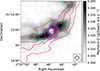 |
Fig. 5. Zeroth-moment map of the region around the NGC 289 absorber NVSS J005245−311503 in greyscale. The map was created by collapsing channels of the r00_t00 data cube between 1708 and 1725 km s−1, corresponding to ±3σ around the CNM central velocity. No masking was applied. Cyan contours show the H I column density at 0.02 and 0.04 Jy beam−1 km s−1 (corresponding to 4.4 × 10²⁰ and 8.8 × 1020 cm−2, respectively). Red contours show velocities of 1692 (southernmost), 1702, 1712, and 1722 km s−1 (northernmost). The pink hatched regions indicate the intersection of the annulus with lines at PA = −55°, which we used to derive the emission spectrum. The r00_t00 beam is shown in the lower right. |
Inspection of the figure shows that the absorber lies behind an H I over-density that crosses it in a roughly south-east to north-west direction. This over-density is part of a larger spiral arm (Fig. 3). The iso-velocity contours run approximately parallel with the filament. Between opposite ends of the absorption feature there is a velocity gradient of ∼15 km s−1. Velocities at these positions are not representative of those at the absorber location. Averaging in, for example, an annulus would result in an artificial broadening of the spectrum. In principle, one could correct for this by removing the rotational signal, and aligning the spectra at the velocity of the absorber, but this would introduce additional assumptions.
We defined a region that follows the observed H I and velocity distribution rather than a purely geometrical model. We selected two regions on either side of the absorber, aligned with the filament and velocity contours. These regions are defined as the intersection of an annulus (inner radius one beam, outer radius two beams) with two parallel lines on either side of the absorber at a position angle of −55°, each offset by one beam. These regions are indicated in Fig. 5. The position angle approximates that of the filament and velocity contours.
In Fig. 6 we show the emission spectrum for these intersection regions as well as that from the full annulus.The difference between full and partial annulus profiles is obvious, and emphasises both the care required in deriving emission spectra and the associated systematic uncertainties.
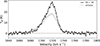 |
Fig. 6. Variation in emission spectra around the absorber NVSS J005245−311503. The grey line shows the average spectrum derived from an annulus with an inner radius equal to one beam width and an outer radius of two beam widths. The black line shows the spectrum derived from the intersection of this annulus with lines at a position angle of −55°. This region is shown in Fig. 4. Note the low-velocity wing in the annulus spectrum, as well as the difference in peak brightness temperature. |
5.1.4. Analysis of the spectra
We first derived the parameters of the absorption spectrum, which is well described by a single Gaussian (as shown in Fig. 4). We obtained a peak optical depth of τ0 = 0.27 ± 0.01, a velocity dispersion of σ0 = 2.90 ± 0.16 km s−1 (FWHM = 6.83 ± 0.38 km s−1) and a central velocity of v0 = 1716.7 ± 0.16 km s−1. These, and other fit parameters discussed later, are listed in Table 2.
Derived properties of the CNM and WNM components along the detected absorption sightlines.
Even though we found a single Gaussian feature, it is possible that it consists of several blended CNM components that are impossible to disentangle at this velocity resolution, so that the fitted profile represents their combined absorption. Here we describe the CNM profile using Eq. (1), with τ(v) given by Eq. (8) for N = 1.
In fitting the observed emission spectrum, we followed the procedure described in Sect. 3, where for the WNM we used Eq. (11), with the number of WNM components K part of the fitting process. With N = 1, the number of trials is limited to 3K.
Determining the number of Gaussian components K is not straightforward. In principle, one could use a goodness-of-fit or information criterion to select the optimal number of components. However, given the limited physical resolution, the observed spectrum is likely only an approximation of the intrinsic emission at the absorber position. It is therefore unclear whether an ‘optimal’ K provides a physically meaningful description. As noted by Murray et al. (2018) and Chen et al. (2025), even small positional offsets can lead to emission components that do not correspond to those seen in absorption.
We used the observed spectrum from the two regions discussed above and shown in Fig. 5. We explored K = 1 and K = 2. The best trials are shown in Fig. 7 for both K values. For K = 1 this is the fit with Fk = 0.0, for K = 2 the fit has Fk = (1.0, 0.5). Although only one representative trial is shown for each K, the parameters listed in Table 2 are weighted averages over all Fk combinations (trials) for that N and K (see Sect. 3), with weights inversely proportional to the variance of each trial.
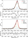 |
Fig. 7. Average emission spectra derived using the regions shown in Fig. 5. The top panel shows the K = 1, Fk = 0 trial. The black line and points indicate the average spectrum. The dashed blue curve shows the CNM emission. The thin dotted black curve shows the intrinsic WNM emission without optical-depth effects. The green curve show the WNM emission, including optical-depth effects, corresponding to gas in behind the absorber. The red curve shows the total (CNM+WNM) emission; residuals are shown in the sub-panel below. Grey lines indicate the zero and ±1σ levels in both panels. The bottom panel shows the K = 2 fit with Fk = (1.0, 0.5). Lines and symbols are as in the top panel. In addition, the orange curve shows the WNM emission in front of the absorber. |
While the K = 2 fits are formally preferred based on the goodness of fit, they introduce emission components that are not well aligned in velocity with the absorption component and yield unrealistically low spin temperatures. This is a consequence of the mismatch between the spatial scales probed by emission and absorption. This effect has been observed even in the MW and the MC, where additional emission components can lead to artificially low inferred spin temperatures. The uncertainty is therefore dominated by mismatches between emission and absorption, rather than by statistical fitting errors. For this reason we also consider the K = 1 fit. It shows larger residuals, but the central velocity of the WNM component agrees to within 0.3 km s−1 with that of the cold component. Given this agreement, as well as the low Ts values and mismatched velocities obtained for K = 2, we conclude that the K = 1 fit provides the most physically meaningful description of the CNM and WNM at the absorber position.
We now discuss how we derived the properties of the CNM and WNM along this sightline. From Eqs. (1) and (6), we found the column density corrected for optical depth effects:
 (15)
(15)
This can be compared with the optically thin expression (Eq. (7)). These values are listed in Table 3. For this line of sight, the ratio of these column densities is 1.036, though this number is likely to be a lower limit, given the resolution effects. We discuss this further in Sect. 6.3.
H I column densities along the absorption lines with and without optical-depth corrections.
5.2. Absorption in NGC 7424
5.2.1. Properties of the galaxy and the continuum source
We detected H I absorption in two sightlines in NGC 7424 (J2257–41). The galaxy is late-type and barred, with an H I disc measuring ∼18 kpc. It hosts the supernova SN2001ig (Ryder et al. 2004, 2006, 2018) and contains a number of strong ultra-luminous X-ray sources (e.g. Soria et al. 2006).
As in NGC 289, the H I and stellar masses (4.0 × 10⁹ and 3.6 × 10⁹ M⊙, respectively) are nearly equal (de Blok et al. 2024), indicating a gas-rich system. Though located in the vicinity of the IC 1459 group (Serra et al. 2015), it is considered to be a field galaxy (Yahil & Vidal 1977; Kourkchi & Tully 2017). We assume a distance of 7.9 Mpc (Leroy et al. 2019), corresponding to 1″ = 0.04 kpc. The first detailed H I observations (obtained with ATCA) were presented in Reeves et al. (2015). NGC 7424 was also observed in H I with KAT-7 by Sorgho et al. (2019). They derived its rotation curve, showing a rapid rise with an extended flat part at around ∼140 km s−1.
The absorption spectra are shown in the central and bottom panels of Fig. 1. The detection towards SUMSS J225729–410241 shows two absorption features at different velocities, likely associated with distinct CNM complexes, and is visible in the r00_t00 zeroth-moment map (Fig. 8). Reeves et al. (2015) also searched for H I absorption against SUMSS J225729–410241, but did not detect any. The absorption feature is visible also in the r05_t00 moment map, but not in the r10_t00 or lower-resolution maps.
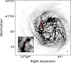 |
Fig. 8. Zeroth-moment map of NGC 7424 based on the r00_t00 data. The red box (1.6′×1.6′) marks the position of the absorption features. The bottom-left inset shows a zoom of this region. The two red ellipses indicate the continuum sources: the larger ellipse marks SUMSS J225729−410241 and the smaller ellipse SN2001ig. The r00_t00 beam is shown in the lower right. |
A second absorption spectrum is detected towards SN2001ig, where absorption occurs against a source within the galaxy rather than a background source. It is not clear whether the absorption is associated with the supernova environment, or whether it is intervening absorption from the H I disc. The SN2001ig absorption feature is not visible in the zeroth-moment map due to the presence of H I emission at higher and lower velocities.
Properties of the two continuum sources are listed in Table 1. For SUMSS J225729–410241, Reeves et al. (2015) find a peak flux of 44.4 ± 1.7 mJy beam−1 at 1.4 GHz (based on their highest resolution data). This is consistent with our measured peak flux of 45.9 mJy beam−1. The source is unresolved and known to be a background QSO (Ryder et al. 2004; Soria et al. 2006). Catalogued as WISEA J225729.67–410239.4, it is also visible in the WISE W1 and W2 bands, but not in W3 and W4. The Legacy Survey shows a counterpart that is significantly redder than the surrounding stellar and star-forming population of NGC 7424.
The second sightline with absorption is towards SN2001ig. This supernova is classified as a Type IIb, and it was notable for the flux modulations in the early aftermath of the explosion, possibly indicating the presence of circumstellar material (Ryder et al. 2004).
Our measured flux density of 10.8 mJy is nearly twice the value of 5.1 ± 0.5 mJy measured ∼700 days after the explosion (Ryder et al. 2004). SN2001ig was observed serendipitously by Reeves et al. (2015). They record 1.4 GHz fluxes of 9.0 ± 0.6 and 8.8 ± 0.7 mJy, for observations done in October 2011 and June 2013 respectively, also suggesting a brightening compared to a decade earlier. If physical, this increase could be due to shock-powered emission associated with the transition from the supernova to the remnant phase. SN2001ig is unresolved in our data. Both sources have been detected in X-ray using Chandra observations (Soria et al. 2006). The projected galactocentric distance of the sources is ∼6.0 kpc.
5.2.2. The absorption spectra
We applied the procedure described in Sect. 5.1.2 to construct an H I-emission-free cube. We used the same robustness parameter of −1, but impose a larger baseline flagging limit of 1500 m, due to the more prominent H I emission in the cube. A complicating factor is the presence of two bright continuum sources (with peak fluxes of ∼0.3 Jy beam−1) in the outer primary beam, about 45′ from the centre. These cause low-level ripples that become prominent in the H I-emission-free cube (where the continuum has not been subtracted), requiring adjustments to the fitting to mitigate their impact. The final emission-free cube has a noise level of 0.64 mJy beam−1.
The absorption towards SUMSS J225729–410241 shows two components (Fig. 9). In quantifying the component parameters, the effect of the ripples meant including a quadratic baseline in the fit, and limiting the fitting range to 820–920 km s−1. The two components have similar properties. The peak optical depths are τ0 = (0.076 ± 0.007, 0.074 ± 0.007). The central velocities v0 are (860.6, 880.3) km s−1. The velocity dispersions of the components are σ0 = (3.46, 2.83) km s−1 [FWHM = (8.13, 6.65) km s−1]. Central velocities and velocity dispersions have very small formal fitting uncertainties. The low-velocity absorption component shows tentative evidence of a small wing on its low-velocity side, but given the presence of the ripple it is difficult to assign a statistical significance to it.
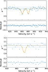 |
Fig. 9. Top: Intrinsic absorption spectrum in NGC 7424 towards SUMSS J225729−410241 derived from the absorption-only data cube. The upper sub-panel shows the spectrum as optical depth τ. The dashed line marks zero optical depth, and the dotted lines indicate the ±1σ levels. Two Gaussian components are overplotted. The lower sub-panel shows the residuals with respect to the fit. Bottom: Absorption spectrum towards SN2001ig. Lines and symbols are as in the top panel. |
The absorption spectrum towards SN2001ig is much fainter (Fig. 9). The continuum ripples necessitate the inclusion of a linear baseline fit and a narrow fitting range of 850–890 km s−1. The absorption spectrum is shown in Fig. 9 and can be described by a single Gaussian component. The most notable property is its narrow velocity width: we find a velocity dispersion of 1.21 ± 0.36 km s−1 (FWHM = 2.84 ± 0.85 km s−1), close to the velocity resolution of our data (1.4 km s−1). The peak optical depth is high, with a value of τ0 = 0.22 ± 0.05. The central velocity is v0 = 867.6 ± 0.3 km s−1. These parameters are summarised in Table 2.
5.2.3. Emission spectra
We again took a detailed look at the spatial variation of the H I column density distribution near the absorbers as well as the velocity field to gauge any possible impact on the derivation of averaged profiles. Figure 10 shows the zeroth-moment map of the area around the absorbers, created by summing the three channels between 866.4 and 867.6 km s−1. This narrow velocity range was chosen to maximise the visibility of the SN2001ig absorption feature. The SUMSS J225729–410241 absorption is also visible despite the velocity range covering only a small part of the feature (see the absorption spectra in Fig. 9).
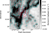 |
Fig. 10. Zeroth-moment map of the region around the NGC 7424 absorbers in greyscale. The map was created by collapsing channels of the r00_t00 data cube between 866.4 and 867.6 km s−1, corresponding to the velocity range of the SN2001ig absorption feature. No masking was applied. Cyan contours show the H I column density at 0.005 and 0.01 Jy beam−1 km s−1 (corresponding to 1.1 × 10²⁰ and 2.2 × 1020 cm−2, respectively). Crosses indicate the positions of the continuum sources. Annuli with inner radius one beam width and outer radius two beam widths are overplotted and bisected by dashed lines at a position angle of −18°. The r00_t00 beam is shown in the lower right. |
The velocity gradient across the absorbers is only a few km s−1, i.e. much smaller than for NGC 289. However, they are located on opposite steep edges of a high–column density H I spiral arm. As was the case for NGC 289, averaging over a full annulus (which includes the spiral arm) yields non-representative emission spectra. To mitigate this we define an annulus around each source, with an inner radius equal to one beam size and an outer radius of two beams. We divide each annulus into two halves using lines at a position angle of −18°, approximating the orientation of the spiral arm. For SUMSS J225729–410241, we use the western (right) part of the annulus to determine the emission spectrum. For SN2001ig we use the eastern (left) part. This avoids including the high-column-density spiral arm in the averaged spectra, as the absorbers are located away from these high column densities. The resulting averaged emission spectra are shown in Fig. 11.
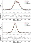 |
Fig. 11. Average emission spectra derived using the regions shown in Fig. 10. The top panel shows the spectrum towards SUMSS J225729−410241, derived from the western half of the annulus. The K = 1, Fk = 0 trial is shown. The black line and points indicate the average spectrum. The dashed blue curves show the two CNM components. The thin dotted black curve shows the intrinsic WNM emission without optical-depth effects. The green curves show the WNM emission including optical-depth effects, corresponding to gas behind the absorber. In the trials displayed here, there is no WNM component in front of the absorbers. The red curve shows the total (CNM+WNM) emission; residuals are shown in the panel below. Grey lines indicate the zero and ±1σ levels in both panels. The bottom panel shows the same for SN2001ig, using the eastern half of the annulus. The K = 1, Fk = 0 trial is shown; lines and symbols are as in the top panel. |
5.2.4. Analysis of the spectra
We fitted the absorption and emission spectra using the same procedure as described in Sect. 5.1.4. For SUMSS J225729–410241 we have two CNM components, i.e. N = 2. For the WNM along this line of sight, a single component (K = 1) is preferred. The combined spectrum is shown in Fig. 11, where we show the Fk = 0 trial. Models with K = 2 or K = 3 do not improve the fit. The figure also illustrates the difficulty of determining the intrinsic emission spectrum in a complex environment with limited spatial resolution. With this single WNM component, the low-velocity CNM component yields a low Ts value. Although the detailed emission profiles and derived CNM and WNM properties vary somewhat with the choice of emission regions, all choices consistently yield a low Ts, reinforcing the earlier conclusion that matching emission and absorption spectra is intrinsically difficult given the different spatial scales probed.
For SN2001ig we have a single CNM component (N = 1) and find that the emission spectrum is best fit with a single WNM component (K = 1). The best-fitting trial with Fk = 0 is shown in Fig. 11. The WNM has a velocity dispersion of ∼9 km s−1 which is a value typically found in the outer parts of H I discs. Models with K = 2 or K = 3 do not lead to quantitatively better fits. The corrections for optical depth are small (but again likely lower limits). All parameters are summarised in Table 2 and 3.
6. Discussion
6.1. Absorption limits
Figure 2 shows that absorption detections are confined to one part of the diagram, approximately defined by Speak ≳ 9 mJy beam−1 and NH II ≳ 7 × 1020 cm−2. To relate the observed H I column densities to the intrinsic gas properties, we correct them for galaxy inclination. The resulting distribution is shown in the top panel of Fig. 12, where we again indicate extended sources, sources associated with Hα, and sources located behind high-inclination galaxies. The bottom panel of Fig. 12 shows only the clean sample, which we consider below.
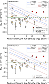 |
Fig. 12. Top: Inclination-corrected H I foreground column density plotted against the peak flux density of the background continuum sources. Red triangles indicate absorption detections. Circles indicate non-detections against unresolved non-Hα sources, filled circles correspond to i < 70°, and open circles correspond to i ≥ 70°. Small stars indicate Hα star-forming regions, and small circles indicate resolved sources not associated with Hα. The filled circles define the ‘clean’ sample of unresolved non-Hα low-inclination sources. The horizontal line marks the Kanekar et al. (2011) threshold at 2 × 1020 cm−2. The dashed diagonal lines show the 3σ absorption detection limits for different Ts and fCNM values. Bottom: same as top, but showing only the clean sample for clarity. |
One factor that can determine whether absorption is detectable is the presence of a CNM phase. In studies of Galactic absorption spectra, Kanekar et al. (2011) find a strong decrease in Ts at NH I ≃ 2 × 1020 cm−2, with higher column densities showing significantly lower temperatures. This transition is interpreted as the onset of CNM formation. Below this threshold, strong absorption is not generally expected.
Figure 12 shows that about two-thirds of the clean sources have foreground column densities below 2 × 1020 cm−2, consistent with the absence of absorption. However, several sources with higher column densities also show no absorption. Reconciling these with a column-density threshold alone would require increasing the threshold to ∼7 × 1020 cm−2, well within the regime where CNM is expected to be present (see Fig. 1 in Kanekar et al. 2011). This suggests that a column-density threshold alone cannot account for the lack of absorption.
This remaining discrepancy is likely related to the optical-depth sensitivity of the data. To derive limits on the H I column density from absorption non-detections, we consider the optical-depth sensitivity. The optical depth is given by τ(v) = − ln(S(v)/Speak), where S(v) is the observed flux density towards the background continuum source in a single spectral channel at velocity v, and Speak is the continuum level measured from line-free channels.
The uncertainty in the optical depth per channel follows from standard error propagation, assuming that the uncertainty in the continuum level is negligible. This gives στ = σI/S(v), where σI is the rms noise per spectral channel in S(v). In the optically thin limit, this expression plays the same role for the uncertainty as Eq. (5) does for the optical depth itself.
In the optically thin limit, S(v)≃Speak and the uncertainty reduces to
 (16)
(16)
To convert the corresponding peak optical-depth limit  into an H I column density limit, we assume a Gaussian absorption profile with FWHM = 2.35 σ. The velocity-integrated optical depth is then ∫τ(v) dv = 1.064 τpeak FWHM. Using Eq. (6) with cf = 1, we obtained
 (17)
(17)
In Sects. 5.1.2 and 5.2.2, we measure σI = 0.41 mJy beam−1 for NGC 289 and 0.64 mJy beam−1 for NGC 7424. We adopt a representative value of σI = 0.5 mJy beam−1 and assume n = 3. We further adopt FWHM = 6 km s−1, corresponding to the average width of the CNM components.
We explored using two different values for the spin temperature. The first is Ts = 20 K, corresponding to the average of our CNM measurements. This lies at the lower end of values derived in the MC (see Dempsey et al. 2022; Chen et al. 2025), and as discussed in Sect. 6.3, it may underestimate the true value. We also considered Ts = 100 K, which is commonly adopted in the literature.
For both Ts values, we calculated the 3σ detection limits as a function of continuum peak flux. As we compare these limits to the total observed H I column densities, we also include a range of fCNM values. The resulting limits are shown in Fig. 12.
For both spin-temperature assumptions, the non-detections are consistent with a lack of optical-depth sensitivity. For Ts = 20 K, this requires fCNM ∼ 0.1, comparable to values found in the SMC (Dempsey et al. 2022). For Ts = 100 K, fCNM ∼ 0.3, typical of the Milky Way (McClure-Griffiths et al. 2023), is sufficient. Reasonable combinations of Ts and fCNM therefore explain most non-detections in terms of limited optical-depth sensitivity.
One exception is the spectrum towards the brightest source, SUMSS J030941−410006 behind ESO 300-G014 (J0309−41). Although it lies above the nominal optical-depth sensitivity limits, its column density is close to the 2 × 1020 cm−2 threshold (Kanekar et al. 2011). Inspection of the spectrum reveals no convincing absorption features (Fig. A.1). A narrow negative spike near 960 km s−1 is inconsistent with a real feature, as it disappears after Hanning smoothing and lies outside the velocity range of the H I emission at that location (911 ± 15 km s−1, derived from the first- and second-moment maps). We therefore conclude that the absence of absorption towards most continuum sources is primarily driven by limited optical-depth sensitivity.
Reeves et al. (2015, 2016) present a search for intervening absorption in 16 nearby gas-rich galaxies using ATCA, including observations of SUMSS J225729−410241 behind NGC 7424. Despite additional observations, no absorption was detected by them. At first glance this may appear surprising, as this is the most prominent absorption feature in the MHONGOOSE sample. Reeves et al. (2015) report a 3σ upper limit on τ0 of 0.09 for their highest-resolution and deepest NGC 7424 data (ATCA-6C array)2. Assuming a FWHM of 10 km s−1, they derive a 3σ upper limit of ∫τ dv = 0.99 km s−1. Using a width of 6 km s−1 instead, comparable to our CNM components, gives an integrated optical-depth limit of 0.59 km s−1. This can be compared with the average integrated optical depth we measure for NGC 7424, which is also 0.59 km s−1. Our detected absorption profiles therefore lie close to the sensitivity limit of the Reeves et al. (2015) data. Their non-detection is thus consistent with the properties of the absorption detected here.
6.2. Stacking
To search for additional absorption in the two galaxies with detected absorption features, we constructed stacked spectra from the r00_t00 emission cubes at the positions of background continuum sources identified with PyBDSF down to 5σcont, where σcont is the noise in the primary-beam-corrected continuum maps. This selection includes sources with flux densities below 0.7 mJy. Within the area covered by the r00_t00 zeroth-moment maps, this yields 120 background sources for J0052−31 and 67 for J2257−41. The rms noise in the continuum images prior to primary-beam correction is 3.0 μJy beam−1 for both fields.
We aligned the spectra to a common velocity frame using the first-moment velocities at each position, assuming that these trace the velocities of the absorption. The H I emission was removed by subtracting Gaussian profile fits with the following constraints: positive amplitude, central velocity within ±30 km s−1, and velocity dispersion between 2.8 km s−1 (two channels) and 50 km s−1. The stacked spectra were constructed as the median of the residual spectra from the 120 and 67 directions, respectively. The resulting rms noise levels are ∼20 μJy and ∼30 μJy for J0052−31 and J2257−41, respectively. These spectra are shown in Fig. 13 and show no absorption features at the 3σ level. The stacked spectrum of J0052−31 shows residual emission near +25 km s−1 at a level just below 3σ. This is likely due to non-Gaussian line shapes in some of the individual spectra.
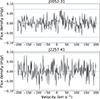 |
Fig. 13. Top: Median stacked spectrum of 120 velocity-aligned sightlines towards continuum sources in NGC 289 (J0052−31). The horizontal lines indicate the zero (dashed), the ±1σ (dotted) and ±3σ (dash-dotted) levels. Bottom: Same but for NGC 7424 (J2257−41), based on 69 sightlines. |
For comparison, we constructed stacked spectra at random positions within the r00_t00 moment maps, i.e. without associated background continuum sources. These spectra show similar noise levels and no evidence of absorption features, consistent with the results above. A more detailed analysis, including (optical-depth-weighted) stacking across the full MHONGOOSE sample, is beyond the scope of this paper.
6.3. Detections
Pingel et al. (2024) present a detailed study of H I absorption in the disc of the Local Group galaxy NGC 6822. Using high-resolution Local Group L-Band Survey (LGLBS) data (Koch et al. 2025), they search for absorption towards 18 sources with peak flux densities > 0.65 mJy beam−1, detecting five CNM components along two lines of sight. No absorption is found towards the remaining sources. In terms of angular resolution, velocity resolution, and sensitivity, this study is comparable to our work. They report a beam of 7.0″ × 5.2″, a channel spacing of 0.4 km s−1, and a channel noise of 7 K. This corresponds to 0.42 mJy beam−1 per 0.4 km s−1 channel, or 0.22 mJy beam−1 when smoothed to 1.4 km s−1, identical to our noise per 1.4 km s−1 channel.
Table 4 compares the CNM properties. While the ranges in linewidth and spin temperature are similar, both the CNM fraction and CNM column density are systematically lower in our sample. Pingel et al. (2024) also find lower CNM fractions than in the MW, MCs, M31, and M33, and interpret this as consistent with evidence that the CNM fraction decreases with metallicity (e.g. Wolfire et al. 1995). Applying this interpretation to our results would imply metallicities for NGC 289 and NGC 7424 lower than the ∼0.2 solar value of NGC 6822, which is unlikely given their higher masses. Walsh et al. (1997) find NGC 289 to be approximately solar metallicity, while NGC 7424 is likely about half solar (Walcher et al. 2006; Modjaz et al. 2011). The systematically lower fCNM and  are therefore more likely due to resolution effects associated with the larger distances of our galaxies (21.5 and 7.9 Mpc versus 0.5 Mpc).
Comparison of CNM properties between this work and Pingel et al. (2024).
The CNM column density is derived from the absorption spectrum (Eq. (6)) and represents a pencil-beam measurement that is independent of galaxy distance. In contrast, quantities such as the total H I column density and fCNM rely on emission spectra, and depend on how representative the emission is of the absorption sightline. These spectra are typically extracted over areas comparable to or larger than the synthesised beam. For Local Group galaxies this corresponds to parsec scales (e.g. ∼15 pc for NGC 6822; Pingel et al. 2024), whereas for more distant systems the same angular resolution corresponds to kiloparsec scales (0.3 and 0.8 kpc for NGC 7424 and NGC 289, respectively).
In the following we adopt a representative physical scale of 0.6 kpc. If the ISM were spatially uniform, changes in scale would have no impact. However, the ISM is structured, with the CNM occupying only a fraction of the projected area, while the WNM is more smoothly distributed (e.g. Soler et al. 2022; Smith et al. 2023; McClure-Griffiths et al. 2023). The structure of the H I can be characterised by the projected fractal dimension Dp, which describes how the area A(L) covered by H I structures scales with size L as A(L)∝LDp. A uniform medium has Dp = 2, while Dp < 2 indicates a clumpy or filamentary morphology. Stanimirovic et al. (1999) measure Dp ≃ 1.5 for the SMC over scales from tens of parsecs to several kiloparsecs. Although this formally applies to total H I, small-scale structure is dominated by cold gas, while the WNM provides a smoother background. Similar values are found for molecular clouds in the MW.
For a beam of size L, the projected CNM covering fraction can be written as
 (18)
(18)
With Dp ≃ 1.5, this gives  . Increasing the beam size by a factor of approximately 40 (from 15 pc to 0.6 kpc) reduces the covering fraction by ∼40−0.5 ≃ 0.16, i.e. a factor of approximately six.
The WNM is distributed on scales larger than L and is largely unaffected. The total observed H I column density can then be written as
 (19)
(19)
When deriving fCNM, the WNM is implicitly assumed to trace the same pencil beam as the CNM. At larger L, this assumption breaks down: much of the WNM emission originates outside the absorption sightline, leading to an overestimate of the WNM contribution and hence to an underestimate of fCNM by a factor of  . Although this is a simplified model, the predicted factor of ∼6 reduction in
  is broadly consistent with the factor of ∼4 difference between our measurements and those of Pingel et al. (2024).
A secondary effect arises in the derivation of the CNM spin temperature. If the emission spectrum includes WNM emission not present along the absorption sightline, the inferred CNM brightness temperature is biased low, leading to lower Ts. Since  scales linearly with Ts, this effect further reduces the inferred CNM column density. The similarity between our results and those of Pingel et al. (2024), suggest both are affected by the same bias.
Finally, the CNM linewidths ΔvFWHM are comparable to those found by Pingel et al. (2024), and the spin temperature ranges largely overlap. This indicates that both studies probe the same class of cold neutral structures. The differences in fCNM and  can therefore be attributed primarily to beam-averaging effects and the sampling of a structured CNM, rather than to intrinsic differences in the gas properties. In addition, the more modest velocity resolution (compared to most MW absorption studies) likely limits the ability to disentangle CNM structures blended in velocity.
6.4. Detection rates
If we assume that the 2 × 1020 cm−2 column density threshold determines whether absorption occurs, we can estimate the fraction of the area of each H I disc above this limit. Using the r00_t00 zeroth-moment maps (with a sensitivity of  cm−2) to define the disc extent, we find that 57 percent of the area in NGC 289 lies above this threshold, with an average disc radius of 54 kpc. For NGC 7424, the corresponding fraction is 54 percent with an average radius of 18 kpc. For the full MHONGOOSE sample, the average fraction is 56%. Thus, for sightlines intersecting the H I disc, absorption would be expected in only slightly more than half of the cases.
We can compare our detection rate with that found by Pingel et al. (2024) for NGC 6822. Their detection rate is also low, with 2 detections in 18 sightlines (11%). This is consistent with our rate of 5% (3/56), or 10% (3/31) for the clean sample. Pingel et al. (2024) note that this is significantly lower than the 38% detection rate found by Dempsey et al. (2022) for the SMC, despite both galaxies being gas-rich, low-mass, and low-metallicity systems. They further mention that all SMC sightlines lie within the 6 × 1020 cm−2 contour. Applying this threshold to NGC 6822 increases the detection rate to 25% (2/8).
Applying the same threshold to the MHONGOOSE data yields a detection rate of 15% (3/20) for all continuum sources behind regions with  cm−2. Excluding sources associated with Hα increases this to 27% (3/11), and restricting further to the clean sample gives 60% (3/5). The inferred detection rate therefore depends strongly on the sample definition. The 6 × 1020 cm−2 contour encloses 0.05 deg2 in NGC 6822 and 0.11 deg2 across all MHONGOOSE galaxies. The two detections in NGC 6822 and three in MHONGOOSE imply comparable detection rates per unit area.
These results show that the detection rate does not depend on sensitivity alone. This complicates extrapolation to blind H I absorption surveys at higher redshift. A key difference is the flux density of the background sources. Our brightest continuum source has a flux of ∼60 mJy, whereas many absorption surveys use sources more than an order of magnitude brighter. This significantly improves optical-depth sensitivity.
As an example, Gupta et al. (2010) study absorption in quasar–galaxy pairs out to z ∼ 0.1. Restricting to the 16 systems with impact parameters < 20 kpc (i.e. likely intersecting the main H I disc; see Reeves et al. 2015, 2016), ∼80% have continuum flux densities > 0.1 Jy and ∼35% exceed 0.5 Jy. Of these, six (∼38%) show H I absorption. For the sightline towards SUMSS J225729−410241, we achieve our best optical-depth sensitivity of στ = 0.014. Assuming a FWHM of 10 km s−1, as in Gupta et al. (2010), this corresponds to a 3σ upper limit of ∫τ dv = 0.45 km s−1. Comparing with the values reported by Gupta et al. (2010), we would have detected only 1–2 of their absorption systems at this sensitivity. This corresponds to a detection rate of 13–26%, significantly lower than their observed rate, and is entirely due to the lower continuum flux densities in our sample. Wide survey areas increase the number of background continuum sources available for absorption searches, but optical-depth sensitivity ultimately determines the fraction of detectable systems (modulo the distribution of absorbing H I within galaxy discs).
7. Summary
We searched for H I absorption towards continuum sources behind the H I discs of the MHONGOOSE galaxies and detected absorption along three lines of sight in two systems, NGC 289 and NGC 7424. With distances an order of magnitude larger than those of Local Group galaxies, the high angular resolution and sensitivity of the MHONGOOSE data allowed the combined emission–absorption method – traditionally applied in the MW and Local Group – to be extended to a new distance regime.
The detections occured along lines of sight with both a high continuum peak flux density and a high foreground H I column density, while other sightlines show no absorption. This can be understood as the combined effect of two factors. First, below a foreground column density of ∼2 × 1020 cm−2, the formation of a substantial CNM component is not expected (Kanekar et al. 2011). Second, optical-depth sensitivity imposes a strict detection limit. Thus, given the sensitivity of our data and the continuum flux densities, many sightlines are either too faint or have insufficient foreground H I to produce detectable absorption.
We compared the derived CNM properties with those from the H I absorption study of NGC 6822 by Pingel et al. (2024), which has comparable sensitivity and resolution. We found CNM column densities and fractions that are lower by a factor of about four. We argue that this difference is not intrinsic but arises from the larger physical scales over which the MHONGOOSE emission spectra are averaged. As a result, the emission spectrum is increasingly dominated by WNM gas unrelated to the narrow absorption sightline, leading to an overestimate of the WNM contribution and an underestimate of fCNM. The similarity in linewidths and spin temperatures between the samples indicates that both studies probe the same class of cold atomic structures and that the observed differences are primarily due to resolution effects.
This study demonstrates that the emission–absorption method can be extended to much larger distances, provided that care is taken in constructing representative emission spectra. This has important implications for future facilities, such as SKA-Mid and the Deep Synoptic Array (Hallinan et al. 2019), which will offer beam sizes smaller by a factor of about two for H I emission compared to this study. This will improve the match between emission and absorption sightlines and reduce systematic biases in derived CNM fractions and spin temperatures. Their increased collecting areas will also enhance optical-depth sensitivity, reducing the reliance on bright background continuum sources. Combined with improved modelling of resolution effects on cold gas distributions, this will enable detailed studies of the CNM and WNM in more distant galaxies.
Acknowledgments
We thank the anonymous referee for the constructive comments. The MeerKAT telescope is operated by the South African Radio Astronomy Observatory, which is a facility of the National Research Foundation, an agency of the Department of Science and Innovation. This work has received funding from the European Research Council (ERC) under the European Union’s Horizon 2020 research and innovation programme (grant agreement No 882793 ‘MeerGas’). FMM carried out part of the research activities described in this paper with contribution of the Next Generation EU funds within the National Recovery and Resilience Plan (PNRR), Mission 4 – Education and Research, Component 2 – From Research to Business (M4C2), Investment Line 3.1 – Strengthening and creation of Research Infrastructures, Project IR0000034 – “STILES – Strengthening the Italian Leadership in ELT and SKA”.
References
- Allison, J. R., Sadler, E. M., Amaral, A. D., et al. 2022, PASA, 39, e010 [NASA ADS] [CrossRef] [Google Scholar]
- Borthakur, S., Momjian, E., Heckman, T. M., et al. 2014, ApJ, 795, 98 [Google Scholar]
- Braun, R., & Walterbos, R. A. M. 1992, ApJ, 386, 120 [Google Scholar]
- Carilli, C. L., & van Gorkom, J. H. 1992, ApJ, 399, 373 [CrossRef] [Google Scholar]
- Chen, H., Stanimirović, S., Pingel, N. M., et al. 2025, AJ, 169, 284 [Google Scholar]
- Condon, J. J., Cotton, W. D., Greisen, E. W., et al. 1998, AJ, 115, 1693 [Google Scholar]
- de Blok, W. J. G., Healy, J., Maccagni, F. M., et al. 2024, A&A, 688, A109 [NASA ADS] [CrossRef] [EDP Sciences] [Google Scholar]
- Dempsey, J., McClure-Griffiths, N. M., Murray, C., et al. 2022, PASA, 39, e034 [NASA ADS] [CrossRef] [Google Scholar]
- Dey, A., Schlegel, D. J., Lang, D., et al. 2019, AJ, 157, 168 [Google Scholar]
- Dickey, J. M., & Brinks, E. 1988, MNRAS, 233, 781 [Google Scholar]
- Dickey, J. M., & Brinks, E. 1993, ApJ, 405, 153 [NASA ADS] [CrossRef] [Google Scholar]
- Dickey, J. M., & Lockman, F. J. 1990, ARA&A, 28, 215 [Google Scholar]
- Dickey, J. M., Brinks, E., & Puche, D. 1992, ApJ, 385, 501 [Google Scholar]
- Dickey, J. M., Mebold, U., Stanimirovic, S., & Staveley-Smith, L. 2000, ApJ, 536, 756 [NASA ADS] [CrossRef] [Google Scholar]
- Dickey, J. M., McClure-Griffiths, N. M., Gaensler, B. M., & Green, A. J. 2003, ApJ, 585, 801 [NASA ADS] [CrossRef] [Google Scholar]
- Dutta, R., Gupta, N., Srianand, R., & O’Meara, J. M. 2016, MNRAS, 456, 4209 [Google Scholar]
- Field, G. B., Goldsmith, D. W., & Habing, H. J. 1969, ApJ, 155, L149 [NASA ADS] [CrossRef] [Google Scholar]
- Gupta, N., Srianand, R., Bowen, D. V., York, D. G., & Wadadekar, Y. 2010, MNRAS, 408, 849 [Google Scholar]
- Gupta, N., Srianand, R., Baan, W., et al. 2016, MeerKAT Science: On the Pathway to the SKA, 14 [Google Scholar]
- Gupta, N., Srianand, R., Farnes, J. S., et al. 2018, MNRAS, 476, 2432 [Google Scholar]
- Hallinan, G., Ravi, V., Weinreb, S., et al. 2019, The DSA-2000– A Radio Survey Camera [Google Scholar]
- Heiles, C., & Troland, T. H. 2003a, ApJS, 145, 329 [Google Scholar]
- Heiles, C., & Troland, T. H. 2003b, ApJ, 586, 1067 [NASA ADS] [CrossRef] [Google Scholar]
- Heywood, I. 2020, Astrophysics Source Code Library [record ascl:2009.003] [Google Scholar]
- Jameson, K. E., McClure-Griffiths, N. M., Liu, B., et al. 2019, ApJS, 244, 7 [NASA ADS] [CrossRef] [Google Scholar]
- Kanekar, N., & Chengalur, J. N. 2003, A&A, 399, 857 [NASA ADS] [CrossRef] [EDP Sciences] [Google Scholar]
- Kanekar, N., Prochaska, J. X., Ellison, S. L., & Chengalur, J. N. 2009, MNRAS, 396, 385 [NASA ADS] [CrossRef] [Google Scholar]
- Kanekar, N., Braun, R., & Roy, N. 2011, ApJ, 737, L33 [NASA ADS] [CrossRef] [Google Scholar]
- Killerby-Smith, N., McClure-Griffiths, N. M., Murray, C. E., & Stanimirović, S. 2025, MNRAS, 538, 2508 [Google Scholar]
- Koch, E. W., Leroy, A. K., Rosolowsky, E. W., et al. 2025, ApJS, 279, 35 [Google Scholar]
- Kourkchi, E., & Tully, R. B. 2017, ApJ, 843, 16 [NASA ADS] [CrossRef] [Google Scholar]
- Lane, W. M. 2000, Ph.D. Thesis, University of Groningen, Netherlands [Google Scholar]
- Leroy, A. K., Sandstrom, K. M., Lang, D., et al. 2019, ApJS, 244, 24 [Google Scholar]
- Liszt, H. 2001, A&A, 371, 698 [NASA ADS] [CrossRef] [EDP Sciences] [Google Scholar]
- Maccagni, F. M., Morganti, R., Oosterloo, T. A., Geréb, K., & Maddox, N. 2017, A&A, 604, A43 [NASA ADS] [CrossRef] [EDP Sciences] [Google Scholar]
- Maina, E. K., Mohapatra, A., Józsa, G. I. G., et al. 2022, MNRAS, 516, 2050 [CrossRef] [Google Scholar]
- Mauch, T., Murphy, T., Buttery, H. J., et al. 2003, MNRAS, 342, 1117 [Google Scholar]
- McClure-Griffiths, N. M., Stanimirović, S., & Rybarczyk, D. R. 2023, ARA&A, 61, 19 [NASA ADS] [CrossRef] [Google Scholar]
- Meurer, G. R., Hanish, D. J., Ferguson, H. C., et al. 2006, ApJS, 165, 307 [NASA ADS] [CrossRef] [Google Scholar]
- Modjaz, M., Kewley, L., Bloom, J. S., et al. 2011, ApJ, 731, L4 [NASA ADS] [CrossRef] [Google Scholar]
- Mohan, N., & Rafferty, D. 2015, Astrophysics Source Code Library [record ascl:1502.007] [Google Scholar]
- Morganti, R., & Oosterloo, T. 2018, A&ARv, 26, 4 [Google Scholar]
- Murray, C. E., Stanimirović, S., Goss, W. M., et al. 2015, ApJ, 804, 89 [CrossRef] [Google Scholar]
- Murray, C. E., Stanimirović, S., Goss, W. M., et al. 2018, ApJS, 238, 14 [NASA ADS] [CrossRef] [Google Scholar]
- Murray, C. E., Stanimirović, S., Heiles, C., et al. 2021, ApJS, 256, 37 [NASA ADS] [CrossRef] [Google Scholar]
- Patra, N. N., Kanekar, N., Chengalur, J. N., & Roy, N. 2018, MNRAS, 479, L7 [Google Scholar]
- Pingel, N. M., Chen, H., Stanimirović, S., et al. 2024, ApJ, 974, 93 [Google Scholar]
- Reeves, S. N., Sadler, E. M., Allison, J. R., et al. 2015, MNRAS, 450, 926 [Google Scholar]
- Reeves, S. N., Sadler, E. M., Allison, J. R., et al. 2016, MNRAS, 457, 2613 [Google Scholar]
- Ryder, S. D., Sadler, E. M., Subrahmanyan, R., et al. 2004, MNRAS, 349, 1093 [NASA ADS] [CrossRef] [Google Scholar]
- Ryder, S. D., Murrowood, C. E., & Stathakis, R. A. 2006, MNRAS, 369, L32 [NASA ADS] [Google Scholar]
- Ryder, S. D., Van Dyk, S. D., Fox, O. D., et al. 2018, ApJ, 856, 83 [NASA ADS] [CrossRef] [Google Scholar]
- Serra, P., Koribalski, B., Kilborn, V., et al. 2015, MNRAS, 452, 2680 [Google Scholar]
- Smith, R. J., Tress, R., Soler, J. D., et al. 2023, MNRAS, 524, 873 [Google Scholar]
- Soler, J. D., Miville-Deschênes, M.-A., Molinari, S., et al. 2022, A&A, 662, A96 [NASA ADS] [CrossRef] [EDP Sciences] [Google Scholar]
- Sorgho, A., Carignan, C., Pisano, D. J., et al. 2019, MNRAS, 482, 1248 [NASA ADS] [CrossRef] [Google Scholar]
- Soria, R., Kuncic, Z., Broderick, J. W., & Ryder, S. D. 2006, MNRAS, 370, 1666 [Google Scholar]
- Stanimirovic, S., Staveley-Smith, L., Dickey, J. M., Sault, R. J., & Snowden, S. L. 1999, MNRAS, 302, 417 [CrossRef] [Google Scholar]
- Walcher, C. J., Böker, T., Charlot, S., et al. 2006, ApJ, 649, 692 [CrossRef] [Google Scholar]
- Walsh, W., Staveley-Smith, L., & Oosterloo, T. 1997, AJ, 113, 1591 [Google Scholar]
- Wolfire, M. G., Hollenbach, D., McKee, C. F., Tielens, A. G. G. M., & Bakes, E. L. O. 1995, ApJ, 443, 152 [Google Scholar]
- Wolfire, M. G., McKee, C. F., Hollenbach, D., & Tielens, A. G. G. M. 2003, ApJ, 587, 278 [Google Scholar]
- Yahil, A., & Vidal, N. V. 1977, ApJ, 214, 347 [NASA ADS] [CrossRef] [Google Scholar]
The values of τpeak and ∫τ dv in Table 8 of Reeves et al. (2015) are consistent only if τpeak is interpreted as the listed value, rather than as a percentage as implied by the column header.
Appendix A: The brightest non-detections
Here we present the spectra of the non-detections towards the 14 brightest continuum sources listed in Table 1. The detection spectra are given in Fig. 1.
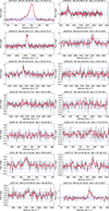 |
Fig. A.1. Spectra of the 14 brightest non-detections as listed in Table 1. Lines and colours as in Fig. 1. |
All Tables
Derived properties of the CNM and WNM components along the detected absorption sightlines.
H I column densities along the absorption lines with and without optical-depth corrections.
All Figures
|
Fig. 1. Spectra of the three absorption profiles. From top to bottom: NVSS J005245−311503 in NGC 289 (J0052−31), SUMSS J225729−410241 in NGC 7424 (J2257−41), and SN2001ig also in NGC 7424 (J2257−41). The original spectra are shown in black, with a five-point Hanning-smoothed version overplotted in red. The 0, ±1σ, and ±2σ levels of the unsmoothed spectrum are indicated by solid, dashed, and dotted lines, respectively. |
| In the text | |
|
Fig. 2. H I emission column densities at the positions of the continuum sources plotted against continuum peak flux. The column densities are not corrected for inclination. Red triangles indicate detections. Circles indicate non-detections towards unresolved non-Hα sources, with filled symbols for i < 70° and open symbols for i ≥ 70°. Small stars indicate Hα star-forming regions, and small circles indicate resolved sources not associated with Hα. Filled circles mark the ‘clean’ sample of unresolved non-Hα sources in low-inclination galaxies. The horizontal dashed line shows the 3σ over 16 km s−1 column density limit of log(NH I/cm−2) = 19.77. |
| In the text | |
|
Fig. 3. Zeroth-moment map of NGC 289 based on the r00_t00 data. The red box in the main panel (1.6′×1.6′) marks the position of the absorption feature. The bottom-left inset shows a zoom-in of this region. The red ellipse indicates the continuum source. The r00_t00 beam is shown in the lower right. |
| In the text | |
|
Fig. 4. Top: Intrinsic absorption spectrum of NVSS J005245−311503 in NGC 289 derived from the absorption-only data cube, shown as optical depth τ. The dashed line indicates zero optical depth, and the dotted lines indicate the ±1σ levels. A single-component Gaussian fit is overplotted. Bottom: Residuals with respect to the Gaussian fit. |
| In the text | |
|
Fig. 5. Zeroth-moment map of the region around the NGC 289 absorber NVSS J005245−311503 in greyscale. The map was created by collapsing channels of the r00_t00 data cube between 1708 and 1725 km s−1, corresponding to ±3σ around the CNM central velocity. No masking was applied. Cyan contours show the H I column density at 0.02 and 0.04 Jy beam−1 km s−1 (corresponding to 4.4 × 10²⁰ and 8.8 × 1020 cm−2, respectively). Red contours show velocities of 1692 (southernmost), 1702, 1712, and 1722 km s−1 (northernmost). The pink hatched regions indicate the intersection of the annulus with lines at PA = −55°, which we used to derive the emission spectrum. The r00_t00 beam is shown in the lower right. |
| In the text | |
|
Fig. 6. Variation in emission spectra around the absorber NVSS J005245−311503. The grey line shows the average spectrum derived from an annulus with an inner radius equal to one beam width and an outer radius of two beam widths. The black line shows the spectrum derived from the intersection of this annulus with lines at a position angle of −55°. This region is shown in Fig. 4. Note the low-velocity wing in the annulus spectrum, as well as the difference in peak brightness temperature. |
| In the text | |
|
Fig. 7. Average emission spectra derived using the regions shown in Fig. 5. The top panel shows the K = 1, Fk = 0 trial. The black line and points indicate the average spectrum. The dashed blue curve shows the CNM emission. The thin dotted black curve shows the intrinsic WNM emission without optical-depth effects. The green curve show the WNM emission, including optical-depth effects, corresponding to gas in behind the absorber. The red curve shows the total (CNM+WNM) emission; residuals are shown in the sub-panel below. Grey lines indicate the zero and ±1σ levels in both panels. The bottom panel shows the K = 2 fit with Fk = (1.0, 0.5). Lines and symbols are as in the top panel. In addition, the orange curve shows the WNM emission in front of the absorber. |
| In the text | |
|
Fig. 8. Zeroth-moment map of NGC 7424 based on the r00_t00 data. The red box (1.6′×1.6′) marks the position of the absorption features. The bottom-left inset shows a zoom of this region. The two red ellipses indicate the continuum sources: the larger ellipse marks SUMSS J225729−410241 and the smaller ellipse SN2001ig. The r00_t00 beam is shown in the lower right. |
| In the text | |
|
Fig. 9. Top: Intrinsic absorption spectrum in NGC 7424 towards SUMSS J225729−410241 derived from the absorption-only data cube. The upper sub-panel shows the spectrum as optical depth τ. The dashed line marks zero optical depth, and the dotted lines indicate the ±1σ levels. Two Gaussian components are overplotted. The lower sub-panel shows the residuals with respect to the fit. Bottom: Absorption spectrum towards SN2001ig. Lines and symbols are as in the top panel. |
| In the text | |
|
Fig. 10. Zeroth-moment map of the region around the NGC 7424 absorbers in greyscale. The map was created by collapsing channels of the r00_t00 data cube between 866.4 and 867.6 km s−1, corresponding to the velocity range of the SN2001ig absorption feature. No masking was applied. Cyan contours show the H I column density at 0.005 and 0.01 Jy beam−1 km s−1 (corresponding to 1.1 × 10²⁰ and 2.2 × 1020 cm−2, respectively). Crosses indicate the positions of the continuum sources. Annuli with inner radius one beam width and outer radius two beam widths are overplotted and bisected by dashed lines at a position angle of −18°. The r00_t00 beam is shown in the lower right. |
| In the text | |
|
Fig. 11. Average emission spectra derived using the regions shown in Fig. 10. The top panel shows the spectrum towards SUMSS J225729−410241, derived from the western half of the annulus. The K = 1, Fk = 0 trial is shown. The black line and points indicate the average spectrum. The dashed blue curves show the two CNM components. The thin dotted black curve shows the intrinsic WNM emission without optical-depth effects. The green curves show the WNM emission including optical-depth effects, corresponding to gas behind the absorber. In the trials displayed here, there is no WNM component in front of the absorbers. The red curve shows the total (CNM+WNM) emission; residuals are shown in the panel below. Grey lines indicate the zero and ±1σ levels in both panels. The bottom panel shows the same for SN2001ig, using the eastern half of the annulus. The K = 1, Fk = 0 trial is shown; lines and symbols are as in the top panel. |
| In the text | |
|
Fig. 12. Top: Inclination-corrected H I foreground column density plotted against the peak flux density of the background continuum sources. Red triangles indicate absorption detections. Circles indicate non-detections against unresolved non-Hα sources, filled circles correspond to i < 70°, and open circles correspond to i ≥ 70°. Small stars indicate Hα star-forming regions, and small circles indicate resolved sources not associated with Hα. The filled circles define the ‘clean’ sample of unresolved non-Hα low-inclination sources. The horizontal line marks the Kanekar et al. (2011) threshold at 2 × 1020 cm−2. The dashed diagonal lines show the 3σ absorption detection limits for different Ts and fCNM values. Bottom: same as top, but showing only the clean sample for clarity. |
| In the text | |
|
Fig. 13. Top: Median stacked spectrum of 120 velocity-aligned sightlines towards continuum sources in NGC 289 (J0052−31). The horizontal lines indicate the zero (dashed), the ±1σ (dotted) and ±3σ (dash-dotted) levels. Bottom: Same but for NGC 7424 (J2257−41), based on 69 sightlines. |
| In the text | |
|
Fig. A.1. Spectra of the 14 brightest non-detections as listed in Table 1. Lines and colours as in Fig. 1. |
| In the text | |
Current usage metrics show cumulative count of Article Views (full-text article views including HTML views, PDF and ePub downloads, according to the available data) and Abstracts Views on Vision4Press platform.
Data correspond to usage on the plateform after 2015. The current usage metrics is available 48-96 hours after online publication and is updated daily on week days.
Initial download of the metrics may take a while.