


| Issue |
A&A
Volume 710, June 2026
|
|
|---|---|---|
| Article Number | L6 | |
| Number of page(s) | 8 | |
| Section | Letters to the Editor | |
| DOI | https://doi.org/10.1051/0004-6361/202659747 | |
| Published online | 28 May 2026 | |
Letter to the Editor
Variability of Sagittarius A* at 3 GHz on minute scales with MeerKAT
1
Max-Planck-Institut für Radioastronomie, Auf dem Hügel 69, 53121, Bonn, Germany
2
Argelander Institute for Astronomy, University of Bonn, Auf dem Hügel 71, 53121, Bonn, Germany
3
Deutsches Zentrum für Astrophysik, Postplatz 1, 02826, Görlitz, Germany
4
Thüringer Landessternwarte, Sternwarte 5, 07778, Tautenburg, Germany
5
Instituto de Astrofísica de Andalucía-CSIC, Glorieta de la Astronomía s/n, E-18008, Granada, Spain
6
Center for Astrophysics | Harvard & Smithsonian, Cambridge, MA, 02138-1516, USA
7
South African Radio Astronomy Observatory, Liesbeek House, River Park, Cape Town, 7705, South Africa
8
Max-Planck-Institut für Gravitationsphysik (Albert Einstein Institute), 30167, Hannover, Germany
9
Leibniz Universität Hannover, 30167, Hannover, Germany
10
SKA Observatory, Jodrell Bank, Lower Withington, Macclesfield, SK11 9FT, United Kingdom
★ Corresponding author: This email address is being protected from spambots. You need JavaScript enabled to view it.
Received:
6
March
2026
Accepted:
24
April
2026
Abstract
The supermassive black hole Sagittarius A* (Sgr A*) exhibits temporal and spectral variability across the electromagnetic spectrum. However, variability at radio frequencies below ∼5 GHz for timescales shorter than a day remains largely unexplored. We investigated the variability of Sgr A* at 2.79 GHz on short timescales (1 min) to probe an under-explored regime of its emission process. Through point-source model fitting in the uv domain, we analysed the flux density variation of Sgr A* over an 8 h observation. We detect flux variation on timescales of a few tens of minutes with a modulation index of 6.11%, a mean flux density of (827 ± 0.1stat ± 33sys) mJy, and a mean spectral slope of 0.08 ± 0.03. Furthermore, we measure the slope of the structure function of the observed light curve to be 0.81 ± 0.05 with a characteristic timescale of about 120 min. Our study at low radio frequencies is a critical step towards constraining the physical mechanisms that drive Sgr A*’s variable emission and its spectral energy distribution. Our study suggests that variability at centimetre and millimetre wavelengths is likely more closely related than previously thought.
Key words: techniques: interferometric / Galaxy: center
© The Authors 2026
 Open Access article, published by EDP Sciences, under the terms of the Creative Commons Attribution License (https://creativecommons.org/licenses/by/4.0), which permits unrestricted use, distribution, and reproduction in any medium, provided the original work is properly cited.
This article is published in open access under the Subscribe to Open model.
Open access funding provided by Max Planck Society.
1. Introduction
The compact source Sagittarius A* (Sgr A*) at the centre of our Galaxy is an ideal candidate for studying supermassive black holes due to its proximity to Earth. A detailed understanding of Sgr A* would provide insight into the interactions of supermassive black holes at centres of distant low-luminosity galaxies with their environments. Brown & Lo (1982) observed its variability at radio frequencies (2695 and 8085 MHz) on both long (years) and short (one day to months) timescales. Multi-wavelength variability has also been observed, with frequent flaring in X-ray (e.g. Baganoff et al. 2001), near-infrared (NIR; e.g. Genzel et al. 2003; Ghez et al. 2004), and radio bands (e.g. Falcke 1999; Wielgus et al. 2022a). The details of the physical mechanisms driving the variability, and the connection between the variability at different wavelengths, remain unclear.
At radio wavelengths, variability is believed to consist of two modes (Yusef-Zadeh et al. 2006; Michail et al. 2021): (1) a flaring component (typically observed on timescales of hours), possibly linked to jets, outflows, magnetic reconnection events, or episodic accretion, and (2) a more stable quiescent component that persists across all timescales, likely associated with a radiatively inefficient accretion disk (see Quataert 2003; Yuan et al. 2003). The rapidly varying flaring component superimposes on the quiescent component, and therefore the radio measurements capture the combined flux from the two states (Michail et al. 2021). Moreover, the spectral energy distribution shows an increase in flux density from radio to sub-millimetre wavebands with a positive spectral slope peaking near 104 GHz, the so-called ‘sub-millimetre bump’ (see e.g. Zylka et al. 1995; Falcke et al. 1998); it drops off sharply in the NIR regime. Falcke (1999) reported variability at 2.3 and 8.3 GHz on timescales of 50–200 days, while Herrnstein et al. (2004) identified epochs of varying flux and spectral index, suggesting the presence of distinct emission states. Variability studies covering a broad frequency range, between 19 and 100 GHz, indicate that the timescale increases at lower frequencies, possibly due to a mildly relativistic outflow (Brinkerink et al. 2015).
We present the first analysis of short-term variability in Sgr A* using MeerKAT radio telescope observations (Jonas 2009) at 2.79 GHz. This relatively unexplored low-frequency regime offers a valuable window into the emission processes. These observations mark the first light curve obtained from our ongoing 200 hr observing campaign dedicated to Sgr A* as part of the MPIfR-MeerKAT Galactic Plane Survey (MMGPS; Padmanabh et al. 2023).
With an intrinsic size of ∼11 mas at 2.79 GHz (based on Eq. (3) from Falcke et al. 2009), the light crossing time is expected to be ∼14 h. We find minute- to hour-scale variability in our 8 h data. We show that the variability at these low frequencies is similar to those found in millimetre observations with the Atacama Large Millimetre/sub-millimetre Array (ALMA; Wielgus et al. 2022a). Our study also demonstrates the power of MeerKAT in studying the variability of Sgr A* with high fidelity, and paves the way for conducting such investigations in greater detail.
2. Temporal properties of Sgr A* at 2.79 GHz
2.1. Light curve and spectral index
In this Letter we analyse light curves of Sgr A* between 2.65 and 3 GHz using data obtained with MeerKAT on 21 March 2024 between UTC 02:17 and 10:07, and investigate flux densities obtained from the uv domain. The observing strategy, data calibration, and flux density extraction are described in Appendix A. Details of the data processing are presented in a separate paper (Rammala-Zitha et al., in preparation).
Figure 1 (top panel) shows the total intensity light curve binned into 1 min intervals over the available bandwidth, while sub-band light curves are shown in Fig. B.1. The sub-band light curves follow a similar trend to the total intensity light curve, with the highest frequency (2.87 GHz) leading the lowest frequency (2.70 GHz). This is quantified in Sect. 2.2. The shaded intervals in all light curve plots correspond to the time samples after t > 08 : 13 UTC, where both the flux density and spectral index vary rapidly; we discuss this interval further in Sect. 3. From here on, we refer to the light curve spanning the full observation as ‘full’ and the light curve excluding samples in the shaded region as ‘excluded’.
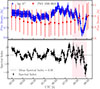 |
Fig. 1. Top panel: Total intensity light curve of Sgr A* in bins of 1 min (blue dots) and the phase calibrator PKS 1830-3602 (red squares) on 21 March 2024 at 2.79 GHz. The error bars include systematic and 1σ statistical uncertainties. Bottom panel: Spectral index (α) variation of Sgr A* over time, derived from sub-band flux measurements. Error bars reflect statistical uncertainties. The dashed line represents the mean α = 0.08 (full). The pink-shaded region indicates the light curve after 08:13 UTC, which shows a rapid decrease in flux density followed by an increase. The data used here are available at the CDS. |
We measure mean flux densities of (827 ± 0.1stat ± 33sys) mJy (full) and (842 ± 0.2stat ± 34sys) mJy (excluded). These measurements are consistent with the flux density of 818 ± 11 mJy measured from the multi-frequency synthesis image, and with literature values (e.g. Bower et al. 2015 at 3 GHz). The modulation index, i.e. the ratio of the standard deviation to the mean flux density, is found to be 6.11 ± 0.38% (full) and 3.50 ± 0.14% (excluded); the uncertainty was estimated as the standard deviation of bootstrap-resampled modulation index values.
To assess the gain stability of the calibration, we plotted the light curve of the gain calibrator PKS 1830−3602 (the red squares the top panel of Fig. 1) in 1 min bins. In contrast to Sgr A*, the calibrator light curve is flat, with a modulation index of 0.8% of the mean flux. This is consistent with a non-variable gain calibrator, confirming the calibration stability and ruling out gain variations as a plausible cause for the observed variability of Sgr A*. Further statistical tests to validate the robustness of the light curve are presented in Appendix C.
We also used the four sub-bands images (∼57 MHz wide) to derive the spectral index. At each timestamp, the flux densities in the four sub-bands were fitted to obtain the spectral index (Sν ∝ να, where Sν is the flux density at frequency ν). Figure 1 (bottom panel) shows the time series of the spectral index (α) in 1 min bins; they range from −4 to +2 (full) and −2 to +2 (excluded). The mean is α = 0.08 ± 0.03 (full) and α = 0.20 ± 0.02 (excluded), consistent with literature measurements (e.g. Iwata et al. 2020; Melia & Falcke 2001; Herrnstein et al. 2004). Figure B.3 shows the spectral index as a function of flux density. It exhibits a bimodal pattern: below 0.75 Jy (coinciding with a dip in the temporal feature towards the end of the observation) the spectrum is steep, while above this threshold no distinctive trend is observed.
2.2. Time lag between sub-bands
We measure a mean spectral index of close to zero, which indicates there may be emission near the transition between optically thick and thin synchrotron emission. In such a scenario, variability can appear at different times across frequencies, making it important to quantify possible delays (van der Laan 1966). To investigate this, we performed a cross-correlation analysis of the light curves at 2.70 and 2.87 GHz and found a time lag of 826 ± 97 s (see Appendix B).
In the optically thick regime, variability could be driven by adiabatic expansion. Assuming expansion of a uniform, spherical blob of synchrotron-emitting plasma of relativistic electrons with energy index p = 2, defined as n(E)∝E−p(Michail et al. 2021), the expected time lag between the two frequencies (based on Eq. 2 in Iwata et al. 2020) is ≈460 s, significantly lower than what we derive (see Fig. B.4). For electrons with strong radiative losses, where p = 4, the time lag is expected to be even lower (≈390 s). Considering a lower p = 1.5, which could arise from reconnection heating, the time lag is expected to be ≈490 s. Thus, our measurement differs by up to a factor of 2, and therefore, variability at 2.79 GHz is unlikely to be caused by adiabatic expansion.
2.3. Structure function
We determined the characteristic timescale of variability from the light curve using a second-order structure function (SF; see Iwata et al. 2020 and references therein). The SF was calculated as SF(τ) = ⟨[Sν(t)−Sν(t+τ)]2⟩, where τ is the time lag. Figure 2 shows that the SF increases to ∼7259.75 s (∼2.02 h) with a slope of 0.81 ± 0.05 (full; blue triangles) and ∼8556.28 s (∼2.38 h) with a slope of 0.80 ± 0.02 (excluded; red circles), as expected for a red-noise process. The flux density distribution (full; Fig. B.2) is asymmetric (Fisher–Pearson skewness of −1.54), with a peak around 0.84 Jy and a tail extending towards lower flux densities (0.65–0.75 Jy). In the SF of the full light curve (blue triangles in Fig. 2), we visually identified a tentative break at a timescale of ≈550 s, below which the slope is 1.22 ± 0.03. Although this timescale is broadly consistent with variability observed at millimetre wavelengths (Wielgus et al. 2022a), we argue that it is not representative of a persistent characteristic timescale. This interpretation is motivated by the presence of a distinct low-flux tail in Fig. B.2, which becomes prominent beginning around 08:13 UTC (highlighted by the pink-shaded region in Fig. 1; top panel). When it is excluded, the SF no longer shows a discernible break (red circles in Fig. 2), and the flux density distribution of the remaining data is well described by a Gaussian (Fisher–Pearson coefficient of 0.45). This suggests that the tail in Fig. B.2 likely reflects a separate physical process, distinct from the main variations captured by the SF, and does not affect the determination of characteristic timescales.
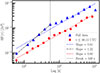 |
Fig. 2. SF of the full light curve (blue triangles) and t ≤ 08 : 13 UTC (red circles). The dashed blue line is the fit to the SF of the full light curve (slope = 0.81). The dashed black line is the fit to the first six data points (slope = 1.22), and the dotted black line indicates the tentative break at 549 s. The dashed red line is the fit to the SF of the t ≤ 08 : 13 UTC light curve (slope = 0.80). |
If the accretion disk around Sgr A* is oriented close to a face-on view (EHT Collaboration 2022a; Wielgus et al. 2022b), the optical depth towards the innermost region may be significantly lower than what a 1D model predicts, and hence the 3 GHz photosphere may be located closer to the black hole. In such a scenario, millimetre and centimetre variability could have similar statistical characteristics, meaning that the observed variability at low frequencies could be caused, in part, by reprocessed emission from mechanisms that drive variability at high frequencies. To test this, we compared the centimetre and millimetre variability of 50 000 simulated light curves that we generated by drawing realizations from a Matérn covariance Gaussian process whose parameters were fitted to the 230 GHz ALMA observations obtained in 2017 (Wielgus et al. 2022a). Each realization was sampled at a cadence of 60 s over a duration of 10 h and initially contained no measurement noise. For each synthetic light curve, we computed the SF after interpolating it onto the observed time grid using logarithmically spaced time-lag bins. To mimic realistic observational conditions, Gaussian noise with a standard deviation of 24 mJy, estimated from the phase calibrator PKS 1830-3602, was added to these synthetic light curves. The slope of the SFs becomes shallower as a result of the addition of noise relative to the noise-free case (see Fig. B.5). The SF slope measured for the first MeerKAT light curve, 0.81 ± 0.05 (full), lies within the distribution obtained from the noise-added simulations, demonstrating consistency with the variability expected from resampling the ALMA light curves to MeerKAT’s cadence.
3. Discussion and conclusion
This study represents the first use of MeerKAT to characterise Sgr A*’s variability and spectral properties. Compared to previous works that used observations widely spaced in time (e.g. Falcke 1999), our high-cadence monitoring provided us with new insights into short-timescale variability at low radio frequencies. Previous studies report a modulation index of 6% at 8.3 GHz and 2.5% at 2.3 GHz (Falcke 1999) on timescale of weeks, whereas we measure 6.11% (full) and 3.5% (excluded) on minute timescales, indicating that similar modulation is already present at shorter timescales.
Our dataset also shows notable peaks and troughs at intervals of ∼20 min (Fig. 1; top panel), prominent from 06:25 UTC onwards. Such short-timescale variability is usually observed at higher frequencies (Genzel et al. 2003; Baganoff et al. 2001; Wielgus et al. 2022a). This suggests that the compact, event-horizon–scale source, known to dominate the millimetre emission of Sgr A* (EHT Collaboration 2022b), also contributes to the variable component at radio frequencies near 3 GHz. Another observed feature is the presence of sudden jumps in flux density, similar to those reported at higher NIR frequencies (Genzel et al. 2003). As seen in Fig. 1, after 08:13 UTC, the light curve exhibits significant changes in flux density. The origin is unclear but may be due to absorption from the opacity effects in the Sgr A* accretion flow. Alternatively, it could arise from outflowing absorption material in the foreground, particularly if the system is observed at a low inclination (EHT Collaboration 2022a; Wielgus et al. 2022b). When considering the light curve up to 08:13 UTC, the bi-modality in the spectral index as a function of flux density is no longer present, indicating that the emission is predominantly optically thick.
One possible origin of the variability seen for Sgr A* is propagation effects of electromagnetic waves in the turbulent interstellar medium, for example via refractive and diffractive scintillation in the strong scattering regime. Following Eqs. 10 and 11 in Psaltis et al. (2018), for Sgr A*, the diffractive timescale (tdif) lies in the range 1 to 4 s, and the refractive timescale (tref) in the range 17–86 yr. These timescales at 10.74 cm, the wavelength of our observations, were estimated assuming that the transverse velocities between the source and the scattering screen are between 10 and 50 km s−1, and that the distance between the potential scattering screen and the observer is 2.7 kpc. Since tdif is smaller than our bin size of 1 min, any diffractive scattering is effectively averaged out. The tref is of the order of years, making it too slow to produce variability on shorter timescales.
Observational evidence of interstellar scattering in the vicinity of Sgr A* is provided by the radio magnetar J1745−2900, located just 3″ from Sgr A*, which exhibits interstellar scattering on a timescale of τsc = 1.3 ± 0.2 s at 1 GHz (Spitler et al. 2014). As τsc ∝ ν−4, this corresponds to τsc < 1 s at 2.79 GHz. Conservatively assuming that the scattering properties along the line of sight to Sgr A* are comparable to those measured towards the nearby radio magnetar J1745−2900, our minute-scale binning is sufficient to wash out the diffractive effects. Hence, the observed variability of Sgr A* is unlikely to be caused by interstellar scattering.
Having ruled out interstellar scattering, we adopted a single-zone model – where a single physical process drives the variability across frequency bands – and performed the time-lag analysis (Sect. 2.2). We find a time delay of 826 ± 97 s, with the light curve at 2.70 GHz lagging behind that at 2.87 GHz. This time lag is somewhat inconsistent with that predicted by the adiabatic expansion scenario, in which the expanding blob of synchrotron-emitting plasma near the vicinity of the accretion disk of Sgr A* becomes optically thin, producing peaks in flux density that occur later at lower frequencies, naturally explaining the observed time delays (Michail et al. 2021). A similar approach was adopted by Wielgus et al. (2022a) at high frequencies (212–230 GHz), where adiabatic expansion models predict lags of order 1–2 min. However, no significant delays were detected, with upper limits ≤10 s. Taken together, these results highlight a frequency-dependent behaviour of Sgr A*, in which the time lag appears to differ between the centimetre (∼3 GHz) and millimetre (∼230 GHz) wavelengths. Although the SF slopes agree, the time lags are significantly different, which makes it difficult to present a consistent, comprehensive scenario. More data, over longer timescales, are needed to study the variability of Sgr A*.
The time delay between the two frequencies could also be determined in the context of the presence of a fast and directed outflow from a relativistic jet of Sgr A* in which the peak frequency of radio emission changes with position along the jet axis (Falcke et al. 2009). Based on the analysis by Brinkerink et al. (2015), the wavelength dependence of the time delay corresponds to a time-lag slope of 36 − 42 min cm−1 based on 100 GHz ALMA data, and 19–48 GHz based on Very Large Array data. For the frequency range between 2.70 and 2.87 GHz, this time-lag slope predicts a lag of ∼24 − 28 min. The measured delay of ∼12 − 15 min is therefore inconsistent with the prediction based on a simplistic jet outflow model that directly relates Very Long Baseline Interferometry sizes and time lags.
The variation in the spectral index contains useful information on changes in the optical depth likely arising from the turbulent accretion flow of plasma around Sgr A* (Wielgus et al. 2022a). In Fig. 1 (bottom panel), we report the spectral index variation over time for Sgr A*. Some fluctuations may also be due to systematic effects, such as the limited bandwidth, which can bias spectral index estimates. Falcke (1999) reported a positive spectral index versus flux density correlation in the centimetre regime. Our spectral index remains independent for flux densities > 0.75 Jy, suggesting that changes in flux density occur without affecting the spectrum, a behaviour also observed at NIR frequencies (Hornstein et al. 2007; Trap et al. 2011; Witzel et al. 2014; Paugnat et al. 2024). If the radio emission is synchrotron, it is more plausible that the variability is driven by changes in the magnetic field strengths and/or the densities of relativistic electrons. However, if the flux density change towards the end of the light curve arises from an absorption feature, this effect alone could explain the observed spectral-index variability. Future observations will help to test these interpretations.
From the SF analysis (Fig. 2), we determined a characteristic timescale of ∼120 min. However, a precise determination of this timescale is difficult from a single light curve, since the SF can be affected by limited sampling. As described in Falcke (1999), the characteristic timescales associated with Sgr A* at these frequencies, including those linked to black hole activity or relativistic outflows, are typically less than a day. Therefore, the timescale of ∼120 min could indicate global accretion flow instabilities. Additionally, Yusef-Zadeh et al. (2011) reported flux variability on sub-minute to hour timescales in their radio data at 8, 22, and 43 GHz, which they attributed to the fact that most of the continuum flux from Sgr A* at radio and sub-millimetre wavelengths is believed to originate within its accretion disk. The first light curve from MeerKAT reported in this Letter indicates variability comparable to that at centimetre and millimetre wavelengths, where the measured SF slope is consistent with the expected values from ALMA light curves. A slower variability would have produced a much steeper slope.
Data availability
The light curve from Figure 1 is available at the CDS via https://cdsarc.cds.unistra.fr/viz-bin/cat/J/A+A/710/L6.
References
- Alexander, T. 1997, in Astronomical Time Series, eds. D. Maoz, A. Sternberg, & E. M. Leibowitz, Astrophys. Space Sci. Lib., 218, 163 [Google Scholar]
- Baganoff, F. K., Bautz, M. W., Brandt, W. N., et al. 2001, Nature, 413, 45 [Google Scholar]
- Bower, G. C., Markoff, S., Dexter, J., et al. 2015, ApJ, 802, 69 [Google Scholar]
- Brinkerink, C. D., Falcke, H., Law, C. J., et al. 2015, A&A, 576, A41 [NASA ADS] [CrossRef] [EDP Sciences] [Google Scholar]
- Brown, R. L., & Lo, K. Y. 1982, ApJ, 253, 108 [Google Scholar]
- CASA Team (Bean, B., et al.) 2022, PASP, 134, 114501 [NASA ADS] [CrossRef] [Google Scholar]
- de Villiers, M. S. 2023, AJ, 165, 78 [Google Scholar]
- EHT Collaboration (Akiyama, K., et al.) 2022a, ApJ , 930, L16 [NASA ADS] [CrossRef] [Google Scholar]
- EHT Collaboration (Akiyama, K., et al.) 2022b, ApJ, 930, L12 [NASA ADS] [CrossRef] [Google Scholar]
- Falcke, H. 1999, in The Central Parsecs of the Galaxy, eds. H. Falcke, A. Cotera, W. J. Duschl, F. Melia, & M. J. Rieke, ASP Conf. Ser., 186, 113 [NASA ADS] [Google Scholar]
- Falcke, H., Goss, W. M., Matsuo, H., et al. 1998, ApJ, 499, 731 [NASA ADS] [CrossRef] [Google Scholar]
- Falcke, H., Markoff, S., & Bower, G. C. 2009, A&A, 496, 77 [NASA ADS] [CrossRef] [EDP Sciences] [Google Scholar]
- Genzel, R., Schödel, R., Ott, T., et al. 2003, Nature, 425, 934 [NASA ADS] [CrossRef] [Google Scholar]
- Ghez, A. M., Wright, S. A., Matthews, K., et al. 2004, ApJ, 601, L159 [CrossRef] [Google Scholar]
- Herrnstein, R. M., Zhao, J.-H., Bower, G. C., & Goss, W. M. 2004, AJ, 127, 3399 [Google Scholar]
- Hornstein, S. D., Matthews, K., Ghez, A. M., et al. 2007, ApJ, 667, 900 [NASA ADS] [CrossRef] [Google Scholar]
- Iwata, Y., Oka, T., Tsuboi, M., Miyoshi, M., & Takekawa, S. 2020, ApJ, 892, L30 [NASA ADS] [CrossRef] [Google Scholar]
- Jankov, I., Kovacevic, A. B., Ilic, D., Sánchez-Sáez, P., & Nikutta, R. 2022, https://doi.org/10.5281/zenodo.7253034 [Google Scholar]
- Jonas, J. L. 2009, IEEE Proc., 97, 1522 [Google Scholar]
- Ludwig, S., & de Villiers, M. 2021, katbeam: Primary beam model library for the MeerKAT project, https://github.com/ska-sa/katbeam?tab=readme-ov-file, accessed: 2024-10-12 [Google Scholar]
- Marti-Vidal, I., Vlemmings, W. H. T., Muller, S., & Casey, S. 2014, UVMULTIFIT: Fitting astronomical radio interferometric data, Astrophysics Source Code Library [record ascl:1402.017] [Google Scholar]
- Melia, F., & Falcke, H. 2001, ARA&A, 39, 309 [Google Scholar]
- Michail, J. M., Yusef-Zadeh, F., & Wardle, M. 2021, MNRAS, 505, 3616 [Google Scholar]
- Offringa, A. R., McKinley, B., Hurley-Walker, N., et al. 2014, MNRAS, 444, 606 [Google Scholar]
- Padmanabh, P. V., Barr, E. D., Sridhar, S. S., et al. 2023, MNRAS, 524, 1291 [NASA ADS] [CrossRef] [Google Scholar]
- Paugnat, H., Do, T., Gautam, A. K., et al. 2024, ApJ, 977, 228 [Google Scholar]
- Psaltis, D., Johnson, M., Narayan, R., et al. 2018, arXiv e-prints [arXiv:1805.01242] [Google Scholar]
- Quataert, E. 2003, Astron. Nachr. Suppl., 324, 435 [Google Scholar]
- Spitler, L. G., Lee, K. J., Eatough, R. P., et al. 2014, ApJ, 780, L3 [Google Scholar]
- Trap, G., Goldwurm, A., Dodds-Eden, K., et al. 2011, A&A, 528, A140 [NASA ADS] [CrossRef] [EDP Sciences] [Google Scholar]
- van der Laan, H. 1966, Nature, 211, 1131 [NASA ADS] [CrossRef] [Google Scholar]
- Wielgus, M., Marchili, N., Martí-Vidal, I., et al. 2022a, ApJ, 930, L19 [NASA ADS] [CrossRef] [Google Scholar]
- Wielgus, M., Moscibrodzka, M., Vos, J., et al. 2022b, A&A, 665, L6 [NASA ADS] [CrossRef] [EDP Sciences] [Google Scholar]
- Witzel, G., Ghez, A. M., Morris, M. R., et al. 2014, ApJ, 796, L8 [NASA ADS] [CrossRef] [Google Scholar]
- Yuan, F., Quataert, E., & Narayan, R. 2003, ApJ, 598, 301 [Google Scholar]
- Yusef-Zadeh, F., Roberts, D., Wardle, M., Heinke, C. O., & Bower, G. C. 2006, ApJ, 650, 189 [NASA ADS] [CrossRef] [Google Scholar]
- Yusef-Zadeh, F., Wardle, M., Miller-Jones, J. C. A., et al. 2011, ApJ, 729, 44 [Google Scholar]
- Zylka, R., Mezger, P. G., Ward-Thompson, D., Duschl, W. J., & Lesch, H. 1995, A&A, 297, 83 [Google Scholar]
Cross-correlations were performed using the pyZDCF package (Jankov et al. 2022), a Python implementation of the Z-transformed discrete correlation function (Alexander 1997).
Appendix A: Observations and data reduction
A.1. Observing strategy
We used the MeerKAT radio telescope to observe Sgr A* using the S4 band receiver (2.62–3.50 GHz) on 21 March 2024 for an on-source time of 7.54 h and a total bandwidth of 875 MHz. These observations were performed as part of the ongoing MMGPS (Padmanabh et al. 2023). The data are observed in nine pointings dithering around Sgr A* (pointing centres shown in Table A.1), with the pointing GC00 is centred on the position of Sgr A*. The observation sequence began with a 5 min scan of the primary calibrator, J1939–6342, followed by a 5 min scan of the polarisation calibrator, 3C 286, and 2 min scans of the secondary (complex gain) calibrator, PKS 1830–3602 interleaved between 20 min scans on the different pointings of Sgr A*. Each of the pointings in Table A.1 were visited twice over the course of the observations run to ensure uniform uv coverage. Another 5 min scan of the primary calibrator was performed at the end of the observations.
Pointing positions used for the observations. Coordinates are given in J2000.
A.2. Calibration and band selection
We used the MMGPS Imaging Pipeline to calibrate the data. We note that, the full width at half maximum of MeerKAT’s primary beam (PB) have complicated frequency-dependent jumps above 3 GHz caused due to the excitation of TM11-mode within the waveguide of the orthomode transducers (de Villiers 2023). This also leads to jumps in the system equivalent flux density. These effects could affect flux density measurements of Sgr A*, particularly for pointings where it is not located at the phase centre. Hence, we discarded data above 3 GHz in our analysis, limiting the bandwidth to 230 MHz at a central frequency of 2.79 GHz. To analyse spectral properties, we sub-divided the available bandwidth into four sub-bands of 57 MHz with central frequencies at 2.70, 2.76, 2.81, and 2.87 GHz.
A.3. Point source fitting
The self-calibrated data set was divided into 1 min intervals using the CASA (CASA Team 2022) tool mstransform to examine the variability of the flux density of the source. We then employed the uvmodelfit tool (Marti-Vidal et al. 2014) in CASA to perform a single-component model fitting to the uv data, estimating the flux density of the source.
A.4. Source isolation and primary beam correction
Given the complexity of the Galactic Centre (GC) environment, characterized by diffuse emission and the presence of the mini-spiral around Sgr A*, we limit our analysis to the large uv distances ≥5 × 10⁴ λ to isolate the emission from Sgr A*. This corresponds to sensitivity to structures smaller than ∼4″, to ensure that only compact emission, dominated by Sgr A*, was included. To further ensure that the uv coverage are the same for all frequencies in our analysis, we used data in the uv range 50 000 to 67 403.3λ.
To correct for the PB, we generated a PB model at the central frequency of 2.79 GHz using KATBEAM (Ludwig & de Villiers 2021). Although the PB remains the same at a particular frequency, the relative position of the source within the beam shifts over time as a result of the dithering of the pointings. To account for this variation, we simulate the motion of the source along a circular trajectory centred on the phase centre at a fixed radial distance. This simulation enabled us to evaluate how minor positional shifts influence the flux correction changes based on the PB response. Specifically, we sampled 100 points along the circular path and estimated the PB correction factor as a function of the azimuth angle for each point. We then calculated the coefficient of variation (standard deviation divided by the mean) of the PB values and incorporated this into flux density uncertainty. This procedure was performed for all four sub-bands.
Appendix B: Flux distribution, the light curves of the sub-bands, and cross-correlation analysis
Here we present the light curves of Sgr A* at 2.70, 2.76, 2.81 and 2.87 GHz (Fig. B.1), the flux density distribution of the light curve at 2.79 GHz (Fig. B.2), spectral index as a function of flux density (Fig. B.3), the cross-correlation plot of the highest (2.87 GHz) and the lowest (2.70 GHz) frequency sub-bands (Fig. B.4), and the histogram of the SF slopes (Fig. B.5).
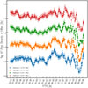 |
Fig. B.1. Total intensity light curves for Sgr A* for four sub-band frequencies (1 min time bins). The light curve of each sub-band is offset by +0.2 onwards from the first sub-band in the flux density for visualization purposes. The error bars include systematic and 1σ statistical uncertainties. The light curves show similar overall trends, with the highest-frequency sub-band (2.87 GHz) leading the lowest-frequency sub-band (2.70 GHz). |
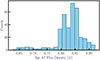 |
Fig. B.2. Distribution of flux densities of Sgr A* at 2.79 GHz in bins of 1 min. The distribution exhibits a distinct maximum at comparatively high flux densities, with an extended tail towards lower values spanning the range of observed flux densities. |
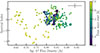 |
Fig. B.3. Variation in the spectral index (α) as a function of flux density of Sgr A* at 2.79 GHz. |
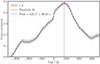 |
Fig. B.4. Cross-correlation amplitude as a function of time lag (τ) between light curves at 2.87 and 2.70 GHz. The grey-shaded band represents the 1 σ uncertainties on the box-car smoothed cross-correlation function. |
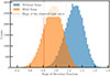 |
Fig. B.5. Histogram of the slopes of the SF for 50 000 synthetic light curves, with and without added noise. The red line marks the slope derived from the observed light curve, which falls within the expected range. |
The cross-correlation1 was calculated as a function of time lag, using a binning scheme with a minimum of 11 points per bin and a maximum lag sampling at half the total duration of the light curve. To assess uncertainties, we performed 1000 Monte Carlo realizations of the cross-correlation curve by randomly perturbing its values within their measurement errors. Figure B.4 shows the cross-correlation function between 2.87 GHz and 2.70 GHz light curves. We determine a time delay of 826 ± 97 s by fitting a second-order polynomial to the peak, obtained by smoothing the cross-correlation function with a boxcar function corresponding to a width of 10 bins. The uncertainty corresponds to the standard deviation of the peak time lags derived from the 1000 Monte Carlo realizations of the smoothed cross-correlation function, generated by propagating the measurement errors provided by pyZDCF.
Appendix C: Verification tests for the Sgr A* light curve
C.1. Test I: Light curve of the calibrator
We generated the light curve of the secondary calibrator PKS 1830−3602 using the same method as that for Sgr A* shown in Fig. 1 (top panel). Since the flux density of PKS 1830−3602 remained relatively stable throughout the observation, any observed trends in the target’s light curve cannot be attributed to instrumental effects, thereby validating our approach. We determine the average flux density of the secondary calibrator to be 2957 ± 118 mJy (where the mean statistical and mean systematic uncertainties are added in quadrature) at 2.79 GHz. It is close to the flux density of PKS 1830−3602 (∼2830 mJy) between 2.877 and 2.962 GHz 2 with a measured modulation index of 0.8%.
We also conducted a spectral index analysis for our secondary calibrator and found it to be relatively constant with a mean spectral index of -1.379 ± 0.004. The variation in the spectral index, as shown in Fig. C.2, is minimal (−1.44 to −1.34 in the uv domain) compared to the significant variation observed for our source, Sgr A*, whose spectral index ranges between −4 to +2.
C.2. Test II: Image domain versus uv domain
We validated our visibility-domain methodology by conducting a similar analysis in the image domain for the secondary calibrator. We imaged all 1 min interval measurement set files using WSCLEAN (Offringa et al. 2014), applying the same uv range and dividing the data into four sub-bands to facilitate spectral index analysis. This approach proved more suitable for the secondary calibrator, which is bright, phase-centred, and situated in a less extreme environment than Sgr A*.
After generating the images, we used the CASA task imfit to extract flux densities and corresponding errors. The resulting light curve appears in Fig. C.1, and the spectral index variation over time is shown in Fig. C.2. Light curves from both the visibility and image domains exhibit consistent trends. The mean flux density is 3042 ± 129 mJy (where the mean statistical and mean systematic uncertainties are added in quadrature), and the mean spectral index is -1.25 ± 0.02.
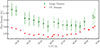 |
Fig. C.1. Comparison of flux density light curves for the secondary calibrator PKS 1830–3602 in the image and visibility domains. We used imfit on images generated in 1 min bins to obtain the green curve, which represents the image-domain flux densities with associated errors. The red curve shows flux densities derived using uvmodelfit in the visibility domain. The error bars represent the 1σ statistical uncertainty. We observe consistent trends between the two methods, validating the robustness of our approach. Differences in error magnitudes reflect the distinct modelling assumptions in each domain. Image-domain errors are larger due to contributions from deconvolution and beam uncertainties, while visibility-domain errors remain smaller because they arise from direct model fitting in the Fourier domain. |
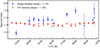 |
Fig. C.2. Spectral index (α) variation of PKS 1830-3602 over time, derived from sub-band flux measurements. Error bars reflect statistical uncertainties. |
This cross-domain comparison also enables a more accurate assessment of error values. Errors in the image domain are ∼100 times smaller than the measured flux density, whereas, in the visibility domain, they are about 10 000 times smaller. The discrepancy likely stems from fewer degrees of freedom in the image domain, where multiple sources are modelled, compared to the single-source model used by uvmodelfit in the visibility domain. Furthermore, image-domain errors include contributions from deconvolution and cleaning, which are absent in the visibility domain.
Discrepancies in flux density values may arise because imfit sometimes fails to properly deconvolve the source from the beam, classifying it as a point source without a reliable size estimate in many snapshots. Gaps in the light curve correspond to failed imfit attempts, often caused by extreme beam elongation that leads to World Coordinate System (WCS) conversion errors, likely due to numerical instability. In particular, the snapshot images for timestamps 9:12:25.5 and 9:13:25.5 are missing, indicating that WSCLEAN did not generate them, and further investigation is needed. The reduced number of data points in the spectral index plot compared to the visibility domain results from imfit failures in individual sub-bands, which prevented spectral index calculation at those times.
C.3. Test III: Light curves of other sources in the field
The analysis in Appendix C.1 demonstrates that the phase calibration solutions have not caused any instrumental time variability. However, it does not rule out any other potential issue restricted only to the target scans. The phase calibrator is always observed at the pointing centre, but Sgr A* is offset from it in most of the GC pointings. The target scans are also self-calibrated, while the phase calibrator is not. Hence, we repeated the analysis for some off-centre point sources in the field of view. For this, we made light curves of these sources, but this time with 5 min binning and visibilities > 30 000λ. This was done in order to gain sufficient signal-to-noise to apply the same uvmodelfit technique as these sources are ∼10 times weaker than Sgr A*. The light curves of these sources, along with Sgr A*, with 5 min binning are shown in Fig. C.3.
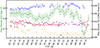 |
Fig. C.3. Total intensity light curve of Sgr A* in bins of 5 min (green dots) and the the other point sources (blue: J1744-2857, red: J1746-2845, orange: J1745-2904, pink: J1746-2856, purple: J1746-2852) on 21 March 2024 at 2.79 GHz. The error bars include systematic and 1σ statistical uncertainties. |
The comparison of 5 min Sgr A* light curve with those of other point sources in the GC shows that none of the point source follows the shape of the light curve obtained for Sgr A*. There are some drop-off points and gaps in the time series for some GC pointings of these sources, indicating that the uv modelling failed, possibly because the sources were right at the edge of the PB in these cases.
From this analysis, the important conclusions are that the short-timescale variations are not seen in other point sources in the GC fields, and the level of fluctuations is smaller than that of Sgr A* even though PB-correction related errors in these sources are relatively higher. Also, based on the phase-calibrator light curve (Fig. 1; top panel), the short-timescale fluctuations due to incorrect amplitude solutions can be ruled out. We also do not see jumps in flux densities of Sgr A* or the point sources across scans. Lastly, the flux densities estimated for 5 min binning for Sgr A* follow the 1 min time bins right on top of each other. All the tests presented in this appendix support the conclusion that the observed light curve variability is unlikely to be caused by instrumental effects related to the dithering of Sgr A* across target scans.
Appendix D: Acknowledgements
We acknowledge Farhad Yusef-Zadeh for initial discussions and helpful insights on this work. This work has made use of the MeerKAT radio telescope, which is operated by the South African Radio Astronomy Observatory, a facility of the National Research Foundation, an agency of the Department of Science and Innovation. This work has benefited from the “MPIfR S-band receiver system”, designed, constructed, and maintained with funding from the MPI für Radioastronomie and the Max Planck Society. In particular, we acknowledge the contributions and efforts of the experts from the Electronics and Digital Signal Processing departments of the MPIfR. MW is supported by a Ramón y Cajal grant RYC2023-042988-I from the Spanish Ministry of Science and Innovation and acknowledges financial support from the Severo Ochoa grant CEX2021-001131-S funded by MCIN/AEI/ 10.13039/501100011033. SR acknowledges the support from the International Max Planck Research School for Astronomy and Astrophysics at the Universities of Bonn and Cologne. RSW and VVK acknowledge support from the European Research Council starting grant COMPACT (Grant agreement number: 101078094).
All Tables
All Figures
|
Fig. 1. Top panel: Total intensity light curve of Sgr A* in bins of 1 min (blue dots) and the phase calibrator PKS 1830-3602 (red squares) on 21 March 2024 at 2.79 GHz. The error bars include systematic and 1σ statistical uncertainties. Bottom panel: Spectral index (α) variation of Sgr A* over time, derived from sub-band flux measurements. Error bars reflect statistical uncertainties. The dashed line represents the mean α = 0.08 (full). The pink-shaded region indicates the light curve after 08:13 UTC, which shows a rapid decrease in flux density followed by an increase. The data used here are available at the CDS. |
| In the text | |
|
Fig. 2. SF of the full light curve (blue triangles) and t ≤ 08 : 13 UTC (red circles). The dashed blue line is the fit to the SF of the full light curve (slope = 0.81). The dashed black line is the fit to the first six data points (slope = 1.22), and the dotted black line indicates the tentative break at 549 s. The dashed red line is the fit to the SF of the t ≤ 08 : 13 UTC light curve (slope = 0.80). |
| In the text | |
|
Fig. B.1. Total intensity light curves for Sgr A* for four sub-band frequencies (1 min time bins). The light curve of each sub-band is offset by +0.2 onwards from the first sub-band in the flux density for visualization purposes. The error bars include systematic and 1σ statistical uncertainties. The light curves show similar overall trends, with the highest-frequency sub-band (2.87 GHz) leading the lowest-frequency sub-band (2.70 GHz). |
| In the text | |
|
Fig. B.2. Distribution of flux densities of Sgr A* at 2.79 GHz in bins of 1 min. The distribution exhibits a distinct maximum at comparatively high flux densities, with an extended tail towards lower values spanning the range of observed flux densities. |
| In the text | |
|
Fig. B.3. Variation in the spectral index (α) as a function of flux density of Sgr A* at 2.79 GHz. |
| In the text | |
|
Fig. B.4. Cross-correlation amplitude as a function of time lag (τ) between light curves at 2.87 and 2.70 GHz. The grey-shaded band represents the 1 σ uncertainties on the box-car smoothed cross-correlation function. |
| In the text | |
|
Fig. B.5. Histogram of the slopes of the SF for 50 000 synthetic light curves, with and without added noise. The red line marks the slope derived from the observed light curve, which falls within the expected range. |
| In the text | |
|
Fig. C.1. Comparison of flux density light curves for the secondary calibrator PKS 1830–3602 in the image and visibility domains. We used imfit on images generated in 1 min bins to obtain the green curve, which represents the image-domain flux densities with associated errors. The red curve shows flux densities derived using uvmodelfit in the visibility domain. The error bars represent the 1σ statistical uncertainty. We observe consistent trends between the two methods, validating the robustness of our approach. Differences in error magnitudes reflect the distinct modelling assumptions in each domain. Image-domain errors are larger due to contributions from deconvolution and beam uncertainties, while visibility-domain errors remain smaller because they arise from direct model fitting in the Fourier domain. |
| In the text | |
|
Fig. C.2. Spectral index (α) variation of PKS 1830-3602 over time, derived from sub-band flux measurements. Error bars reflect statistical uncertainties. |
| In the text | |
|
Fig. C.3. Total intensity light curve of Sgr A* in bins of 5 min (green dots) and the the other point sources (blue: J1744-2857, red: J1746-2845, orange: J1745-2904, pink: J1746-2856, purple: J1746-2852) on 21 March 2024 at 2.79 GHz. The error bars include systematic and 1σ statistical uncertainties. |
| In the text | |
Current usage metrics show cumulative count of Article Views (full-text article views including HTML views, PDF and ePub downloads, according to the available data) and Abstracts Views on Vision4Press platform.
Data correspond to usage on the plateform after 2015. The current usage metrics is available 48-96 hours after online publication and is updated daily on week days.
Initial download of the metrics may take a while.