| Issue |
A&A
Volume 688, August 2024
|
|
|---|---|---|
| Article Number | L12 | |
| Number of page(s) | 12 | |
| Section | Letters to the Editor | |
| DOI | https://doi.org/10.1051/0004-6361/202451146 | |
| Published online | 06 August 2024 | |
Letter to the Editor
General relativistic effects and the near-infrared variability of Sgr A*
II. A systematic approach to temporal asymmetry
1
Max-Planck-Institute für Radioastronomie, Auf dem Hügel 69, 53121 Bonn, Germany
2
University of Illinois, Urbana-Champagne, USA
3
Italian ALMA Regional Centre, INAF-Istituto di Radioastronomia, Via P. Gobetti 101, 40129 Bologna, Italy
4
Max Planck Institut for Extraterrestrial Physics, 85748 Garching bei Muenchen, Germany
5
Physics and Astronomy Department, University of California, Los Angeles, CA 90095-1547, USA
6
Center for Astrophysics | Harvard & Smithsonian, 60 Garden Street, Cambridge, MA 02138, USA
7
Department of Physics, TUM School of Natural Sciences, Technical University of Munich, 85748 Garching, Germany
Received:
17
June
2024
Accepted:
9
July
2024
Abstract
A systematic study, based on the third-moment structure function, of Sgr A*’s variability finds an exponential rise time, τ1,obs = 14.8−1.5+0.4 minutes, and decay time, τ2,obs = 13.1−1.4+1.3 minutes. This symmetry of the flux-density variability is consistent with earlier work, and we interpret it as being caused by the dominance of Doppler boosting, as opposed to gravitational lensing, in Sgr A*’s light curve. A relativistic, semi-physical model of Sgr A* confirms an inclination angle of i ≲ 45°. The model also shows that the emission of the intrinsic radiative process can have some asymmetry even though the observed emission does not. The third-moment structure function, which is a measure of the skewness of the light-curve increments, may be a useful summary statistic in other contexts of astronomy because it senses only temporal asymmetry; that is, it averages to zero for any temporally symmetric signal.
Key words: acceleration of particles / accretion, accretion disks / Galaxy: center
Corresponding author; This email address is being protected from spambots. You need JavaScript enabled to view it.
© The Authors 2024
 Open Access article, published by EDP Sciences, under the terms of the Creative Commons Attribution License (https://creativecommons.org/licenses/by/4.0), which permits unrestricted use, distribution, and reproduction in any medium, provided the original work is properly cited.
This article is published in open access under the Subscribe to Open model.
Open access funding provided by Max Planck Society.
1. Introduction
Ever since the detection of the near-infrared (NIR) and X-ray counterpart (Baganoff et al. 2001; Genzel et al. 2003) of the radio source Sgr A*, the source’s variability at all wavelengths has been the subject of intense study. Sgr A*’s NIR light curve shows occasional bright outbursts, typically phenomenologically referred to as flares. An NIR flare is always present when an X-ray outburst occurs (Eckart et al. 2008), but the converse is not true; only a fraction of bright NIR flares are accompanied by an X-ray flare (e.g., Dodds-Eden et al. 2009). Even when flares occur in both bands, the respective flux levels are not highly correlated (e.g., GRAVITY Collaboration 2021). The spectral shape of NIR to X-ray flares has now been established to be rising in the NIR as νLν ∝ ν+0.5 and falling in the X-ray as νLν ∝ ν−0.5 (Hornstein et al. 2007; Yusef-Zadeh et al. 2009; Ponti et al. 2017; GRAVITY Collaboration 2021).
Modern interferometric observatories can detect Sgr A* at all times (GRAVITY Collaboration 2020a), which reveals that Sgr A* is a constantly variable source even in the absence of higher flux peaks (flares). This NIR variability has been studied in detail: the source shows stochastic, red-noise-like behavior akin to many other compact objects (e.g., Do et al. 2009). The power spectrum shows no features and breaks into uncorrelated white noise on timescales of ≈150 minutes (e.g., Witzel et al. 2012, 2018). The RMS–flux relation is linear with no significant difference in variability for bright and faint parts of the light curve, again very similar to other compact objects Witzel et al. 2012; GRAVITY Collaboration 2020a; Weldon et al. 2023). On the other hand, the NIR flux distribution is log-right-skewed; that is, it shows a tail with respect to a log-normal distribution (Dodds-Eden et al. 2009; Witzel et al. 2012; GRAVITY Collaboration 2020a). This tail is typically used to motivate the concept of flares as events in the accretion flow, contrasting with the quiescent condition.
If flares are modeled as distinct events, two types of one-zone models can describe the data. One type peaks at submillimeter wavelengths and produces NIR and X-ray flux through synchrotron self-Compton (SSC) emission (e.g., Eckart et al. 2008; Yusef-Zadeh et al. 2009; Witzel et al. 2021). In the other type, both the NIR and X-ray emission are caused entirely by synchrotron emission, and the resulting but unobserved SSC emission peaks at gamma-ray energies. Models of the first type require enormous electron densities to obtain sufficient SSC flux to reproduce the X-ray spectral index, and therefore are often disfavored (Dodds-Eden et al. 2011; Ponti et al. 2017; GRAVITY Collaboration 2021).
An additional observational input to models is that the astrometry of NIR flares can be tracked. Observed flares show close-to-circular proper motions in the sky, the so-called orbital motions (GRAVITY Collaboration 2018, 2020b). In addition, NIR flares show characteristic loop-like swings in linear polarization (GRAVITY Collaboration 2020c, 2023). These NIR observations were corroborated by EHT–ALMA observations (Wielgus et al. 2022; Event Horizon Telescope Collaboration 2022a), which detected a similar polarization loop in the 230 GHz light curve immediately after a bright X-ray flare. The astrometric behavior supports the notion of flares having an event-like character, whereby flares are interpreted as orbiting “hot spots” in the accretion flow.
If the flare motion is interpreted as an accelerating point-particle orbiting Sgr A*, orbital parameters such as the radius and the viewing angle can be constrained. Both the NIR data and the submillimeter polarization loop (Wielgus et al. 2022) are consistent with a face-on inclination. The Sgr A* EHT image also indicates that the accretion flow is viewed face-on (Event Horizon Telescope Collaboration 2022a,b,c,d,e,f). Thus, there are four independent indications that Sgr A*’s accretion flow is oriented face-on: NIR astrometry of flares, NIR polarization of flares, radio polarization of the light curve after an NIR flare, and the EHT image of Sgr A*.
Paper I (von Fellenberg et al. 2023) analyzed light curves obtained in the NIR (4.5 micron, Spitzer) and in the X-ray (2–8 keV, Chandra, XMM-Newton). On average, Sgr A* flares are well approximated by a double-sided, symmetric, exponential profile with a rise and decay time τ ≈ 15 min. For a fully relativistic and ray-traced orbiting hot-spot model (GRAVITY Collaboration 2020b), such a profile can only be explained if gravitational lensing in the light curve is not important; that is, if the orbits are viewed face-on. In this picture, the symmetry of the average flare shape is explained by dominant Doppler-boosting as the hot spot orbits. When averaged over several flares, the different initial orbital positions lead to symmetric Doppler amplification of the underlying emission. The symmetric flare shape is a fifth, independent constraint on the viewing angle of Sgr A*. This constraint uses only the variability and the assumption of moving hot spots close to Sgr A*. This constraint therefore applies to all hot-spot models, as the variability induced by such a moving hot spot is valid for any radiative model of the underlying emission mechanism, as any close-to-circular motion close to Sgr A* will be lensed and boosted.
A limitation in paper I was the arbitrary selection of flares, their flux normalization, and the shifting and adding applied. This paper generalizes the analysis by first establishing summary statistics to measure asymmetry based on flux differences. Section 3 introduces a statistical model to measure asymmetry in a stochastic process, and Section 4 applies the method to fit the observed Sgr A* light curves (Section 2). Section 5 introduces a semi-physical general-relativistic model and uses it to derive intrinsic Sgr A* properties consistent with the observed light curves, and Section 6 puts the results in context. All fits to data make use of the approximate Bayesian computation (ABC) method described in subsection 4.3.
2. Data
Our data consist of eight NIR observations by Spitzer/IRAC, each ∼24 continuous hours, observed from 2013 to 2017. The timing resolution is 8.4 seconds, which we re-binned to a cadence of 1 minute. Throughout this paper, we use data that are not corrected for extinction; that is, we use observed flux densities. This choice makes no difference to our results except for overall normalization of light curves. The data are public (Witzel et al. 2018, 2021), and the calibration approach was explained by Hora et al. (2014). As those authors explain, the flux density zero point is unknown, but that makes no difference for this paper.
3. Light curves and structure functions
To characterize the statistical properties of light curves, this paper uses flux-density differences of pairs of points separated by a given time lag, τ. This is a common approach in astronomy (e.g., Simonetti et al. 1985). Figure 1 illustrates the underlying concept: for each time-lag, τ, all available flux pairs in a light curve are measured and histogrammed. Then the statistical moments of each histogram, here the mean (μ1), the variance (μ2), and the (Fischer) skewness (μ3), are calculated. The value of any of these moments as a function of the time lag, τ1, is the structure function:
 (1)
(1)
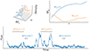 |
Fig. 1. Cartoon showing the concept of moment-based summary statistics for light-curve analysis. The bottom panel shows an example light curve. The orange and blue annotation indicates the flux differences for two given time lags, τ1 and τ2. The top panel shows the histogram of flux differences for every time lag, τi. Each histogram has its respective statistical moments: mean (μ1), variance (μ2), and skewness (μ3). At the upper right, variance and skewness are plotted as functions of time lag. |
where c is a normalization constant. For practical reasons, and to increase the fidelity of the estimate, time lags are grouped in bins, τi, of suitable width in τ.
3.1. The second-moment structure function
The vast majority of astronomical works use the second-moment (variance) structure function, μ2 = σ2. Different normalizations have been used in the literature, but a standard formula for the unnormalized SF (SFμ2, e.g., Simonetti et al. 1985) is
![Mathematical equation: $$ \begin{aligned} \mathrm SF^{\prime } _{\mu _2}(\tau _{i}) = \frac{1}{N_{i}}\sum _{t_{j}, t_{k}}[F(t_{j}) - F(t_{k})]^{2},~ \tau _{i} < (t_{j} - t_{k}) \le \tau _{i+1}. \end{aligned} $$](/articles/aa/full_html/2024/08/aa51146-24/aa51146-24-eq4.gif) (2)
(2)
Here, N is the number of data pairs in each time-lag bin, i, and F(tj)−F(tk) is the difference in flux density between times tj and tk.
For this work, we normalized the structure-function to the interval SF(τ)∈[0, 1]:
 (3)
(3)
which is identical to definition in Equation (2) up to the factor 1/4σ2(F), where σ2(F) is the variance of the light curve. This choice of normalization renders the SFμ2 dimensionless, does not depend on the absolute flux levels, and measures only the correlation in the data. This can be understood when a mathematical property of the second-moment structure function is taken into account. The structure function forms a Fourier pair of the power spectrum of a light curve (a consequence of Parceval’s theorem des Chênes 1799), and this normalization removes the absolute value of the power spectrum. Therefore, SFμ2 is sensitive only to the slope of the power spectrum.
3.2. The third-moment structure function
Following the logic of SFμ2, the third moment of the flux density differences, the skewness, μ3, defines the unnormalized third-moment structure function,
![Mathematical equation: $$ \begin{aligned} \mathrm SF^{\prime } _{\mu _3}(\tau _i) = \frac{1}{N_{i}} \sum _{t_{j}, t_{k}}[F(t_{j}) - F(t_{k})]^{3} ,\end{aligned} $$](/articles/aa/full_html/2024/08/aa51146-24/aa51146-24-eq6.gif) (4)
(4)
with the same symbols as in Equation (2). To obtain a unit-free normalization in the interval SFμ3(τ)∈[0, 1], we applied
 (5)
(5)
where σ2(F) denotes the variance of the light curve, and μ3(F) denotes its Fischer skewness (e.g., Joanes & Gill 1998), defined as
![Mathematical equation: $$ \begin{aligned} \mu _3 = \frac{E[(X-\mu )^3]}{E[(X-\mu )^2]^{3/2}}, \end{aligned} $$](/articles/aa/full_html/2024/08/aa51146-24/aa51146-24-eq8.gif) (6)
(6)
where E stands for the expectation value. As for SFμ2(τ), this dimensionless normalization ensures that the third-moment structure function is sensitive only to the asymmetry in the flux differences and is not dependent on the slope of the power spectrum.
The third-moment structure functions possess several useful properties illustrated in Figure 21. The third-moment structure function shows a negative sign for positively skewed flares and a negative sign for negatively skewed flares. For symmetrical flares, the skewness function is approximately zero for all time lags. Similarly, white noise, which is added to all curves, is approximately zero, on average, in any one realization.
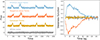 |
Fig. 2. Illustration of the properties of SFμ3(τ). The left panel shows four artificial light curves of different types as labeled, and the right panel shows their skewness functions defined by Equation (5). |
Thus, the SFμ3(τ) is sensitive only to asymmetric signals, and white noise averages to zero when there are enough data points. These properties make the third-moment structure function a versatile metric for astronomical signals that are intrinsically asymmetric (e.g., QPEs Arcodia et al. (2021), eclipsing binaries Gautam et al. (2024), ...).
4. Quantifying asymmetry in light curves
4.1. An intuitive overview of the method
While μ3 (Equation (6)) easily quantifies asymmetry in a distribution of measurements (or random numbers), it is not immediately apparent how asymmetry can be understood for a time series. For a singular event, asymmetry can easily be defined by whether the left and right flanks around the event’s peak are identical (symmetric) or not (asymmetric). While an event is not a probability distribution, the mathematical formalism to calculate the third moment can be applied, and a positive or negative skew will translate into positive or negative SFμ3(τ) (Equation (5)) values. What works for a single peak must also work for repeating, isolated events, and asymmetry is easily probed in that case by the sign of SFμ3(τ), as is illustrated in Figure 2. We discuss a proper definition of symmetry under time reversal in Appendix C and proof that in the case of symmetry the third-moment structure function is zero. The sign of the SFμ3(τ) also probes asymmetry for different light curve types, including when individual flares are less isolated and overlap or when no easy definition of an individual event is apparent.
The difficult part of using SFμ3(τ) to measure asymmetry in a light curve is quantifying the asymmetry and its statistical significance. Any light curve can be split up into segments, some of which will, by chance, show positive or negative values of SFμ3(τ). As for any statistic, with fewer data pairs, the moment, μ3, of the flux difference distribution becomes less well determined. The following sections establish a method to quantify the significance of asymmetry in the light curve based on the Moving Average (MA) model for time series. This model allows generic symmetric and asymmetric light-curve generation as well as an easy definition of the magnitude of asymmetry and its significance. This approach has largely been inspired by the discussion of Scargle (2020), who discussed the utility of MA models for astronomy.
4.2. Moving average model
The MA model is a generic way of generating a stationary light curve (e.g., Priestley 1988; Scargle 1981, 2020). Following the notation of Scargle (2020), a light-curve point, X(n), at time step, n, is given by
 (7)
(7)
where ck are the MA coefficients called the “impulse response” of the process. R(n) are uncorrelated random numbers at each time step, k, typically called the “innovation”, and D(n) is a deterministic function. Effectively, this can be expressed as the convolution of the random process, R(n), with the impulse response, C:
 (8)
(8)
It can be shown that, for a suitable choice of ck and R(n), the MA model is capable of representing any stationary light curve (Wold theorem: Wold 1964; Scargle 2020). The MA is therefore suitable for generating mock light curves depending only on the choice of impulse response, the chosen distribution of random numbers, and the luck of the actual random numbers generated.
In generating mock light curves, the random numbers, R(n), need not be drawn from a uniform distribution. Again following Scargle (2020), we chose a β-distribution; that is, a random variable, x, drawn from uniformly distributed random numbers, 𝒰 ∈ [0, 1], generates
 (9)
(9)
Choosing α = 0 gives white noise. Figure B.1 demonstrates the effect of larger values of α: α = 10 leads to a nonuniform, but not highly skewed, distribution of random values, R. This, when convolved with the kernel, C, leads to a light curve in which individual events are hardly distinguishable. Higher values of α lead to more skewed innovations and more distinct individual events in the light curve.
The choice of kernel, C, is arbitrary, and while it can be measured from the data, it is difficult to find a good kernel a priori. Paper I showed that flares of Sgr A* are well represented, at least on average, by a double exponential function. In particular, Paper I used a PCA decomposition of stacked flares to obtain a de-noised kernel, derive a τ+/− ∼ 15 minutes, and show that PCA can differentiate different kernel shapes for a broad range of MA model parameters. This motivates our choice of a doubled-sided exponential parameterized by τ1 and τ2 for the impulse response:
 (10)
(10)
This choice has the advantage that 1) the MA model can be fit to the light-curve data using the structure functions discussed in section 3, and 2) the asymmetry in the light curve can be expressed as Δτ = τ1 − τ2. The uncertainties of the values, τ1, τ2, and Δτ, can be derived from the posteriors of the model fit.
4.3. Parameter estimation by approximate Bayesian computation
To find what values of τ1 and τ2 best fit the observed light curves, we used the ABC approach. The model requires two additional parameters, α, and an overall flux-density normalization, fscale. Specifically,
 (11)
(11)
where 𝒰α is the innovation shown here convolved with Cobs(τ1,obs,τ2,obs), the observed impulse response defined above, and fscale is the normalization constant. The amplitude of the measured noise in the rebinned light curves, σobs, and process median, M(F), are known in advance and need not be solved for, but each model light curve requires a random realization of the measured noise, 𝒩(σobs.).
The model parameters were constrained using the PYABC code (Klinger et al. 2018; Schälte et al. 2022), which minimizes the distance between the summary statistics of the data and of the model. Our choice of unit-free normalization for both structure functions causes a selective parameter sensitivity in the numerical problem
-
SFμ2(τ) mostly constrains the average width of the kernel, ⟨τ⟩≡(τ1 + τ2)/2;
-
SFμ3(τ) mostly constrains the impulse response difference, Δτ ≡ (τ2 − τ1).
To constrain α and fscale, we included a third summary statistic – namely, the Kolmogorov–Smirnov (KS) test - to estimate the difference between model and data flux distributions. Table B.1 gives an overview of model parameters and the chosen priors.
4.4. Light-curve asymmetry results
Sgr A*’s observed light curve in the NIR can be successfully modeled with an almost symmetric kernel, with an average rise and decay time of τ ≈ 15 minutes. Table B.1 lists the model parameters, their uninformative priors, and the resulting posteriors. Figure 3 illustrates example light curves and impulse responses, which are all nearly symmetric. The result is consistent with that of paper I, where only the shape of the average flares in the light curve was modeled. In particular, the constraints on the rise and fall time are
 (12)
(12)
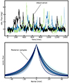 |
Fig. 3. Top: one real and three mock light curves. The colored lines show mock light curves generated with the MA model and best-fit posteriors. The black line shows a segment of an observed Sgr A* light curve. Bottom: Kernel functions constructed using τ1, 2 drawn from the MA-model posterior. |
and there is no significant difference between the rise and fall times of Sgr A*’s observed impulse response, Cobs.
5. General relativistic effects
5.1. A semi-physical relativistic Sgr A* model
The intrinsic variability of Sgr A* is modified by relativistic effects, such as Doppler boosting and relativistic lensing. To explore these, we used the so-called “orbiting hot-spot model” in which bright flares are caused by a localized zone moving in the accretion flow. The flares are assumed to move on bound orbits around the black hole and are boosted and lensed depending on the observer viewing angle and the position in the orbit. Magnifying effects comprise both Doppler boosting and lensing. Both are inclination-angle dependent and are minimum for face-on orbits. Increasing the inclination angle increases both effects but by differing amounts. At i < 30°, lensing is negligible, but for i > 50°, lensing dominates. In addition, lensing is “faster,” leading to a distinct magnification peak that is broadened by the “slower” boosting contribution.
For this work, magnifications were calculated from a ray-traced image library (GRAVITY Collaboration 2018). The model is relativistic, albeit with a fast-light approximation (for discusion see e.g., Porth et al. 2019). Figure 4 illustrates the effects for two inclination angles. A high inclination (i.e., an edge-on view) leads to asymmetric peaks in the magnification, and hence in the light curve, and the asymmetry shows up in a characteristic dependence of SFμ3(τ) on τ. A low inclination leads to smaller, symmetric boosts in magnification, and SFμ3(τ) is near zero for all τ.
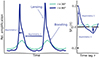 |
Fig. 4. Relativistic magnification in Sgr A*’s light curve. The left graph shows the magnification kernel computed from a library of ray-traced images GRAVITY Collaboration (2020b) for two different inclination angles, as is indicated by the line colors. The time interval plotted is two orbits. Both lensing and boosting peak at the orbit phase near 1.5π (Hamaus et al. 2009). The right graph shows SFμ3(τ) computed for each magnification curve using Equation (13). |
In order explore the relativistic effects, we constructed a semi-physical model for Sgr A*’s light curve:
 (13)
(13)
The first part in Equation (13) represents a shot-noise model. This models the light curves as a sequence of flares, where the number of flares is drawn from a Poisson distribution with rate rf. The flare amplitudes are drawn from an inverse gamma distribution2 with parameters α, β. GRn(t, i) is the relativistic magnification kernel. To obtain the relativistic magnification for each flare, we assumed that the flares occur uniformly around the black hole with a distance from the black hole drawn from a Gaussian distribution (mean 8Rg, SD 1Rg, bounded at [6Rg, 10Rg]). The intrinsic emission of the flare was modeled with a double-exponential kernel function, Cint(t,τ1,int,τ2,int), as in Equation (10), but the intrinsic rise and fall times in general will differ from the observed ones. The second part in Equation (13) was added to account for low-level variance in the data, typically referred to as the quiescence emission (e.g., Dodds-Eden et al. 2009). In order to model this quiescence emission, we used a generic time series model: the exponentiated Ohrnstein–Uhlenbeck (AR1) process, which is identical to a first-order AR model (AR1). This process models the overall data structure well and is by definition temporally symmetric (Witzel et al. 2018).
Our model does not try to model the radiative emission mechanism. This is a limitation because the radiative process itself may well produce asymmetry in the light curve. Examples include adiabatic expansion (e.g., Yusef-Zadeh et al. 2009) and radiative cooling (e.g., Aimar et al. 2023). Nevertheless, the model constrains the asymmetry of the intrinsic emission (modeled by Cint[t, τ1, int, τ2, int]), though the intrinsic emission could be more asymmetric than the observed emission if the asymmetry induced by relativistic effects happens to cancel the intrinsic asymmetry. The actual model fit, like the one in section 4.3, was via the ABC algorithm.
5.2. Derived Sgr A* properties
The cumulative flux distribution, as well as the second- and third-moment structure function, are well described by the model, as is illustrated in Figure 5. Light curves generated from the posterior distribution qualitatively match the observed light curves of Sgr A* (Figure 6).
 |
Fig. 5. Summary statistics from posterior samples (blue) of the converged model fit compared to real observations (black). Statistics are shown separately for the eight observed light curves. The left panel shows the cumulative flux-density distribution, and the other two panels show the two structure-function distributions, as is labeled. |
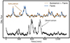 |
Fig. 6. Simulated light curve draw from the model posterior compared to a differential light curve measured by Spitzer. The blue line shows simulated flares (first part in Equation (13)) drawn from the flare-model posterior. The brown line shows the full model light curve including the quiescence emission and observational noise, and the black line shows a Spitzer observation. The curves are vertically offset for clarity, but the y axis has the same linear scale for both curves. |
In the context of the model, high-inclination viewing angles are ruled out (Figure 7). This is because  shows no significant deviation from zero, which is inconsistent with the characteristic swing for high inclinations (Figure 4).
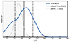 |
Fig. 7. Inclination posterior of the relativistic model. The blue line shows the derived posterior, the gray line shows the inclination posterior of GRAVITY Collaboration (2023), and the gray-shaded region shows the constraints derived from the 230 GHz image of the EHT Collaboration Event Horizon Telescope Collaboration (2022a). |
Furthermore, the best fit shows no dip in SFμ2(τ), which would correspond to a peak in the power spectrum. This means the fit does not require significant periodicity, despite the flares being modeled as orbiting hot spots. This is a consequence of the low flare rate and the different initial orbital positions. In addition, the preferred low inclinations cause only weak relativistic boosting, and therefore little orbital modulation. Finding an orbiting hot-spot model with no periodicity proves that the absence of significant periodicity is not evidence against the orbiting hot-spot model itself but is rather a consequence of the model parameters.
The fit also allows for the intrinsic timescales to be longer than the observed timescales (Section 4.2), as is shown in Figure 8. This illustrates the “speeding up” of timescales by relativistic magnification. The speedup can also be quantified by the overall variance of the model light curves, which are altered by the magnification to show more and sharper peaks. This can be quantified by comparing posteriors with the same random seeds but with relativistic effects set to either zero or one. The overall light curve variance is decreased by ∼20% by the relativistic effects.
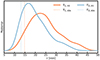 |
Fig. 8. Posteriors of intrinsic timescales. Colored curves show posteriors of τ1,int (orange) and τ2,int (blue) derived from fitting the relativistic model. Vertical dashed lines show the timescales (τ1,obs and τ2,obs, colors as labeled) in the observed light curves as derived from fitting the MA model. |
6. Discussion and summary
This paper extends the results from Paper I, which showed that the average shape of Sgr A*’s NIR and X-ray flares is symmetric. The present work confirms this symmetry in the entire light curve. The average observed rise and fall times are τ1, obs ≈ τ2, obs ≈ 15 minutes.
It is surprising that Sgr A*’s overall light curve shows no significant asymmetry because the radiative processes thought relevant for Sgr A* are typically asymmetric. For instance, variability caused by electron-synchrotron cooling or adiabatic expansion after an initial acceleration event produces skewed light curves (e.g., Dodds-Eden et al. 2009; Aimar et al. 2023; Michail et al. 2024).
Paper I demonstrated that Doppler boosting of an orbiting hot spot can plausibly explain the symmetry in Sgr A*’s flares. While individual events may have strong asymmetry, depending on the starting position of the hot spot in the orbit, the boosting averaged over multiple independent hot spots will be symmetric. Paper I also showed that hot spots in edge-on orbits produce asymmetric flares because of lensing. Such orbits are therefore inconsistent with the observed flare symmetry. This paper corroborates these results by modeling the light curve with a semi-physical, relativistic model, composed of orbiting flares on top of a correlated red-noise-like quiescence emission. The intrinsic process may be more asymmetric than the observed emission because of the averaging over orbits, but our model fits the observations only if i ≲ 45° (Figure 7). This is consistent with other observations, which give stricter constraints.
Lastly, Sgr A*’s light curves have a red-noise-like character with no significant periodicity. Nevertheless, our models show that orbiting hot spots in the accretion flow are consistent with these light curves. The absence of significant periodicity is explained by a combination of short intrinsic timescales, low inclinations, a low flare rate, and flares erupting at random orbit phases (i.e., at uniformly distributed orbit positions).
The third-moment structure function is a useful statistic for a wide variety of astronomical studies because many astronomical signals are temporally asymmetric. Examples include astrometric signatures of orbiting black holes (El-Badry et al. 2023a,b), light curves of eclipsing binaries (Ott et al. 1999; Gautam et al. 2024), and even gravitational-wave signals (Abbott et al. 2019). These examples illustrate the utility of the third-moment structure function well beyond the topic of this paper.
There have been attempts to use modifications of the structure-function to measure asymmetry in light curves (e.g., Kawaguchi et al. 1998; Hawkins 2002; Chen & Wang 2015), non of which probe temporal asymmetry directly. Shishov & Smirnova (2005) used an asymmetry function to probe the flux density distributions of pulsars for interstellar scintillation, which, however, does not probe temporal asymmetry. Weisskopf et al. (1978) use a time-asymmetry function, based on Frenkiel & Klebanoff (1967), which can also probe temporal asymmetry.
The choice of a gamma distribution was motivated by the observed flux-density distribution GRAVITY Collaboration (2020a).
Acknowledgments
The authors thank the referee for their constructive and very fast report which improved the manuscript. H.-H. Chung is supported for this research by the International Max-Planck Research School (IMPRS) for Astronomy and Astrophysics at the University of Bonn and Cologne. This publication is part of the M2FINDERS project which has received funding from the European Research Council (ERC) under the European Union’s Horizon 2020 Research and Innovation Programme (grant agreement No 101018682).
References
- Abbott, B. P., Abbott, R., Abbott, T. D., et al. 2019, Phys. Rev. X, 9, 031040 [Google Scholar]
- Aimar, N., Dmytriiev, A., Vincent, F. H., et al. 2023, A&A, 672, A62 [NASA ADS] [CrossRef] [EDP Sciences] [Google Scholar]
- Arcodia, R., Merloni, A., Nandra, K., et al. 2021, Nature, 592, 704 [NASA ADS] [CrossRef] [Google Scholar]
- Baganoff, F. K., Bautz, M. W., Brandt, W. N., et al. 2001, Nature, 413, 45 [Google Scholar]
- Beaumont, M. 2010, Ann. Rev. Ecol. Evol. Syst., 41, 379 [CrossRef] [Google Scholar]
- Chen, X.-Y., & Wang, J.-X. 2015, ApJ, 805, 80 [NASA ADS] [CrossRef] [Google Scholar]
- des Chênes, P. 1799, Sciences, mathématiques et physiques (Savants étrangers) [Google Scholar]
- Do, T., Ghez, A. M., Morris, M. R., et al. 2009, ApJ, 691, 1021 [NASA ADS] [CrossRef] [Google Scholar]
- Dodds-Eden, K., Porquet, D., Trap, G., et al. 2009, ApJ, 698, 676 [NASA ADS] [CrossRef] [Google Scholar]
- Dodds-Eden, K., Gillessen, S., Fritz, T. K., et al. 2011, ApJ, 728, 37 [NASA ADS] [CrossRef] [Google Scholar]
- Eckart, A., Schödel, R., García-Marín, M., et al. 2008, A&A, 492, 337 [CrossRef] [EDP Sciences] [Google Scholar]
- El-Badry, K., Rix, H.-W., Cendes, Y., et al. 2023a, MNRAS, 521, 4323 [NASA ADS] [CrossRef] [Google Scholar]
- El-Badry, K., Rix, H.-W., Quataert, E., et al. 2023b, MNRAS, 518, 1057 [Google Scholar]
- Event Horizon Telescope Collaboration (Akiyama, K., et al.) 2022a, ApJ, 930, L12 [NASA ADS] [CrossRef] [Google Scholar]
- Event Horizon Telescope Collaboration (Akiyama, K., et al.) 2022b, ApJ, 930, L13 [NASA ADS] [CrossRef] [Google Scholar]
- Event Horizon Telescope Collaboration (Akiyama, K., et al.) 2022c, ApJ, 930, L14 [NASA ADS] [CrossRef] [Google Scholar]
- Event Horizon Telescope Collaboration (Akiyama, K., et al.) 2022d, ApJ, 930, L15 [NASA ADS] [CrossRef] [Google Scholar]
- Event Horizon Telescope Collaboration (Akiyama, K., et al.) 2022e, ApJ, 930, L16 [NASA ADS] [CrossRef] [Google Scholar]
- Event Horizon Telescope Collaboration (Akiyama, K., et al.) 2022f, ApJ, 930, L17 [NASA ADS] [CrossRef] [Google Scholar]
- Frenkiel, F. N., & Klebanoff, P. S. 1967, Phys. Fluids, 10, 507 [NASA ADS] [CrossRef] [Google Scholar]
- Gautam, A. K., Do, T., Ghez, A. M., et al. 2024, ApJ, 964, 164 [NASA ADS] [CrossRef] [Google Scholar]
- Genzel, R., Schödel, R., Ott, T., et al. 2003, Nature, 425, 934 [NASA ADS] [CrossRef] [Google Scholar]
- GRAVITY Collaboration (Abuter, R., et al.) 2018, A&A, 618, L10 [NASA ADS] [CrossRef] [EDP Sciences] [Google Scholar]
- GRAVITY Collaboration (Abuter, R., et al.) 2020a, A&A, 638, A2 [NASA ADS] [CrossRef] [EDP Sciences] [Google Scholar]
- GRAVITY Collaboration (Bauböck, M., et al.) 2020b, A&A, 635, A143 [CrossRef] [EDP Sciences] [Google Scholar]
- GRAVITY Collaboration (Jiménez-Rosales, A., et al.) 2020c, A&A, 643, A56 [CrossRef] [EDP Sciences] [Google Scholar]
- GRAVITY Collaboration (Abuter, R., et al.) 2021, A&A, 654, A22 [NASA ADS] [CrossRef] [EDP Sciences] [Google Scholar]
- GRAVITY Collaboration (Abuter, R., et al.) 2023, A&A, 677, L10 [NASA ADS] [CrossRef] [EDP Sciences] [Google Scholar]
- Hamaus, N., Paumard, T., Müller, T., et al. 2009, ApJ, 692, 902 [NASA ADS] [CrossRef] [Google Scholar]
- Hawkins, M. 2002, MNRAS, 329, 76 [NASA ADS] [CrossRef] [Google Scholar]
- Hora, J. L., Witzel, G., Ashby, M. L., et al. 2014, ApJ, 793, 120 [NASA ADS] [CrossRef] [Google Scholar]
- Hornstein, S. D., Matthews, K., Ghez, A. M., et al. 2007, ApJ, 667, 900 [NASA ADS] [CrossRef] [Google Scholar]
- Joanes, D. N., & Gill, C. A. 1998, J. R. Stat. Soc.: Ser. D (Stat.), 47, 183 [Google Scholar]
- Kawaguchi, T., Mineshige, S., Umemura, M., & Turner, E. L. 1998, ApJ, 504, 671 [NASA ADS] [CrossRef] [Google Scholar]
- Klinger, E., Rickert, D., & Hasenauer, J. 2018, Bioinformatics, 34, 3591 [CrossRef] [Google Scholar]
- Michail, J. M., Yusef-Zadeh, F., Wardle, M., et al. 2024, ApJ, submitted [arXiv:2406.01671] [Google Scholar]
- Ott, T., Eckart, A., & Genzel, R. 1999, ApJ, 523, 248 [NASA ADS] [CrossRef] [Google Scholar]
- Ponti, G., George, E., Scaringi, S., et al. 2017, MNRAS, 468, 2447 [NASA ADS] [CrossRef] [Google Scholar]
- Porth, O., Chatterjee, K., Narayan, R., et al. 2019, ApJS, 243, 26 [Google Scholar]
- Priestley, M. B. 1988, Non-linear and Non-stationary time Series Analysis (Academic Press), 237 [Google Scholar]
- Scargle, J. D. 1981, ApJS, 45, 1 [NASA ADS] [CrossRef] [Google Scholar]
- Scargle, J. D. 2020, ApJ, 895, 90 [NASA ADS] [CrossRef] [Google Scholar]
- Schälte, Y., Klinger, E., Alamoudi, E., & Hasenauer, J. 2022, J. Open Source Software, 7, 4304 [CrossRef] [Google Scholar]
- Shishov, V. I., & Smirnova, T. V. 2005, Astron. Rep., 49, 905 [NASA ADS] [CrossRef] [Google Scholar]
- Simonetti, J. H., Cordes, J. M., & Heeschen, D. S. 1985, ApJ, 296, 46 [NASA ADS] [CrossRef] [Google Scholar]
- von Fellenberg, S. D., Witzel, G., Bauböck, M., et al. 2023, A&A, 669, L17 [NASA ADS] [CrossRef] [EDP Sciences] [Google Scholar]
- Weisskopf, M. C., Sutherland, P. G., Katz, J. I., & Canizares, C. R. 1978, ApJ, 223, L17 [NASA ADS] [CrossRef] [Google Scholar]
- Weldon, G. C., Do, T., Witzel, G., et al. 2023, ApJ, 954, L33 [NASA ADS] [CrossRef] [Google Scholar]
- Wielgus, M., Moscibrodzka, M., Vos, J., et al. 2022, A&A, 665, L6 [NASA ADS] [CrossRef] [EDP Sciences] [Google Scholar]
- Witzel, G., Eckart, A., Bremer, M., et al. 2012, ApJS, 203, 18 [NASA ADS] [CrossRef] [Google Scholar]
- Witzel, G., Martinez, G., Hora, J., et al. 2018, ApJ, 863, 15 [NASA ADS] [CrossRef] [Google Scholar]
- Witzel, G., Martinez, G., Willner, S. P., et al. 2021, ApJ, 917, 73 [NASA ADS] [CrossRef] [Google Scholar]
- Wold, H. 1964, Econometric Model Building (Amsterdam: North-Holland) [Google Scholar]
- Yusef-Zadeh, F., Bushouse, H., Wardle, M., et al. 2009, ApJ, 706, 348 [NASA ADS] [CrossRef] [Google Scholar]
Appendix A: Properties of the third-moment structure function
The third-moment structure function SFμ3 measures asymmetry. Figure A.1 demonstrates that for an exponential impulse-response kernel, the structure function has a characteristic functional form. In particular, the larger the asymmetry (difference between rise and fall time), the stronger the signal in SFμ3. Because of the normalization, the structure function depends only on the time difference in the rise and decay times, not the amplitude of the kernel.
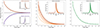 |
Fig. A.1. Third-moment structure functions SFμ3 for different kernels constructed from double-exponential profiles (Equation 10). Insets show example kernels, and the curves in the main panel show the resulting SFμ3. Left: Symmetric (gray) and asymmetric (positive in orange, negative in blue) kernels. Middle: Five kernels with a fixed rise time τ1 = 15 and fall times τ2 = 15 (symmetric), 20, 25, 30, and 35. The larger SFμ3 values correspond to longer fall times as indicated by the curves’ color saturation. Right: Asymmetric kernels of different amplitudes. All have rise times τ1 = 15 and fall times τ2 = 30, but amplitudes are multiplied by 1, 2, 3, 4, and 5. The structure function is the same for all amplitudes. |
Figure A.2 demonstrates how the SFμ2(τ) function reacts to correlated noise. The three panels show light curve realizations generated with the same asymmetric impulse response and identical random seeds but different exponents α of the innovation (Equation 9). The longer the light curve, the better different SFμ3(τ) functions approximate the functional form of the skewness function of the impulse response. For shorter light curves, the errors are largest at large lag times, where there are fewer sample pairs, and fewer samples suffice when α is large because events are less blended. Regardless of the correlation in the noise, if the sufficient data are available, the SFμ3(τ) function recovers the temporal asymmetry in the data. This demonstrates its utility: even correlated noise does not bias the results, especially at short lag times.
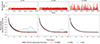 |
Fig. A.2. Simulated light curves and derived structure functions. Upper panels: Light curves for different values of α (Equation 9) as labeled. The light curves were generated by the MA model (Equation 7) and include random and correlated noise with the random seed the same for all panels. The kernels are double-exponential profiles (Equation 10), and the innovation R = Uα was drawn from uniformly distributed samples in [0, 1). Colors at the left mark sections of the light curve with 5 000 and 50 000 samples with the full curves containing 500 000. Lower panels: Structure functions of the simulated light curve above each panel. The black curve shows the true structure function without noise. The colored curves show the structure function derived from each light curve with a finite number of samples as labeled. |
Appendix B: Models and fitting
Figure B.1 illustrates the properties of light curves generated from an MA model. The figure shows the kernel function (C(t, τ1, τ2) (impulse response) in the top panel. The middle panel shows three realizations of the innovation 𝒰α for α = 1000, 100, and 10 respectively. The higher the value of α, the more the distribution is skewed. The bottom panel shows the light curves generated from such a process. The higher α the more “isolated” flares appear in the light curve, while for low α the concept of flare seems ill defined. Nevertheless, the underlying impulse response is the same.
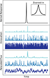 |
Fig. B.1. Simulated light curves generated based on the MA model. Top: temporally symmetric kernel response function. Middle: innovation R(α) for sparse, intermediate, and dense random impulses with α = 1000, 100, and 10, respectively. Bottom: the light-curve products convolved from the kernel and the corresponding innovation processes. Light curves are normalized by their maximal flux value for demonstration. |
B.1. Model parameters, priors, and posteriors
Table B.1 gives the model parameters, priors, and posteriors.
Model parameters, priors, and posteriors for the MA model and semi-physical Sgr A* model.
B.2. Distance functions and model convergences
We used three distance functions for the likelihood inference. The second-moment structure function of the simulated data was compared to the observed data using a distance function akin to the log χ2 function:
 (B.1)
(B.1)
The third-moment structure function of the simulated data was compared to observed data using a distance function akin to the χ2 function:
 (B.2)
(B.2)
which accounts for the fact that the third-moment structure function can have positive as well as negative values. The time lags were binned using 3 minute linear time bins, which was the empirically determined optimum between time sampling and noise in the structure functions.
For the MA model, we used the classical KS test to compare observed and simulated flux distributions. The test turned out to be too insensitive to correctly model the tail of the flux distribution for the semi-physical Sgr A*. For the latter, we used cumulative (flux distribution) histogram fitting as a distance function, where we calculated the χ2 distance between the histogram’s bins.
We employed the population Monte Carlo (PMC) algorithm (Beaumont 2010) implemented in abcpy, which converges using ‘populations’ of random samples, which are iteratively generated, with each generation posing tight constraints on the parameters. One practical convergence criterion is that more generations do not lead to substantially different constraints on the derived parameters. We illustrate that this is the case for both the generic MA model, as well as for the semi-physical relativistic Sgr A*, in the following.
B.2.1. MA model
Figure B.2 illustrates that we have run the abcpy’s PMC long enough to derive meaningful parameter constraints. The quantities of the distribution do not change substantially between the second-last generation and the last.
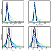 |
Fig. B.2. Posterior for the model (Equation 11) generated using the approximate Bayesian computation (ABC) method. The different colored lines indicate different “sample generations”, with darker colors representing more converged chains. |
B.2.2. Relativistic Sgr A* model
As for the MA model, Figure B.3 illustrates that the alogrithm has run for sufficient time to be considered converged.
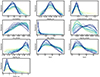 |
Fig. B.3. Same as Figure B.2, but for the convergences behavior of the of the relativistic Sgr A* model. Dark colors indicate later populations. |
Appendix C: Proof of SFμ3 asymmetry properties
We would like to show that for a temporally symmetric light curve, SFμ3 = 0.
Let {F1(t)} be a stationary random process with t = 0, ±1, ±2, ... and {F2(t)} a second stationary random process with F2(−t) = F1(t) for all t. Let us define SFμ3(τ) and  to be the respective structure functions (see definition Equation 2).
Then,
 (C.1)
(C.1)
i.e., time reversal leads to a change of sign of the third-moment structure function.
In this paper, we define temporal symmetry not in the sense of a deterministic function (i.e., F(t) = F(−t)), but in a statistical sense. This can be achieved by adopting a definition similar to the definition of stationarity, as given by Priestley (1988):
Definition. The random process {F1(t)} is said to be statistically time-symmetric up to order m if, for any admissible t1, t2, ..., tn, all the joint moments up to order m of {F1(t1),F1(t2),...,F1(tn)} exist and equal the corresponding joint moments up to order m of {F2(t1),F2(t2),...,F2(tn)}, with F2(t) = F1(−t) for all t.
Then also all the corresponding moments on time-lag selected differences are equal, e.g., SFμ3 =  . If the third-moment order structure functions are equal and negative to one another, their values have to be zero.
All Tables
Model parameters, priors, and posteriors for the MA model and semi-physical Sgr A* model.
All Figures
|
Fig. 1. Cartoon showing the concept of moment-based summary statistics for light-curve analysis. The bottom panel shows an example light curve. The orange and blue annotation indicates the flux differences for two given time lags, τ1 and τ2. The top panel shows the histogram of flux differences for every time lag, τi. Each histogram has its respective statistical moments: mean (μ1), variance (μ2), and skewness (μ3). At the upper right, variance and skewness are plotted as functions of time lag. |
| In the text | |
|
Fig. 2. Illustration of the properties of SFμ3(τ). The left panel shows four artificial light curves of different types as labeled, and the right panel shows their skewness functions defined by Equation (5). |
| In the text | |
|
Fig. 3. Top: one real and three mock light curves. The colored lines show mock light curves generated with the MA model and best-fit posteriors. The black line shows a segment of an observed Sgr A* light curve. Bottom: Kernel functions constructed using τ1, 2 drawn from the MA-model posterior. |
| In the text | |
|
Fig. 4. Relativistic magnification in Sgr A*’s light curve. The left graph shows the magnification kernel computed from a library of ray-traced images GRAVITY Collaboration (2020b) for two different inclination angles, as is indicated by the line colors. The time interval plotted is two orbits. Both lensing and boosting peak at the orbit phase near 1.5π (Hamaus et al. 2009). The right graph shows SFμ3(τ) computed for each magnification curve using Equation (13). |
| In the text | |
|
Fig. 5. Summary statistics from posterior samples (blue) of the converged model fit compared to real observations (black). Statistics are shown separately for the eight observed light curves. The left panel shows the cumulative flux-density distribution, and the other two panels show the two structure-function distributions, as is labeled. |
| In the text | |
|
Fig. 6. Simulated light curve draw from the model posterior compared to a differential light curve measured by Spitzer. The blue line shows simulated flares (first part in Equation (13)) drawn from the flare-model posterior. The brown line shows the full model light curve including the quiescence emission and observational noise, and the black line shows a Spitzer observation. The curves are vertically offset for clarity, but the y axis has the same linear scale for both curves. |
| In the text | |
|
Fig. 7. Inclination posterior of the relativistic model. The blue line shows the derived posterior, the gray line shows the inclination posterior of GRAVITY Collaboration (2023), and the gray-shaded region shows the constraints derived from the 230 GHz image of the EHT Collaboration Event Horizon Telescope Collaboration (2022a). |
| In the text | |
|
Fig. 8. Posteriors of intrinsic timescales. Colored curves show posteriors of τ1,int (orange) and τ2,int (blue) derived from fitting the relativistic model. Vertical dashed lines show the timescales (τ1,obs and τ2,obs, colors as labeled) in the observed light curves as derived from fitting the MA model. |
| In the text | |
|
Fig. A.1. Third-moment structure functions SFμ3 for different kernels constructed from double-exponential profiles (Equation 10). Insets show example kernels, and the curves in the main panel show the resulting SFμ3. Left: Symmetric (gray) and asymmetric (positive in orange, negative in blue) kernels. Middle: Five kernels with a fixed rise time τ1 = 15 and fall times τ2 = 15 (symmetric), 20, 25, 30, and 35. The larger SFμ3 values correspond to longer fall times as indicated by the curves’ color saturation. Right: Asymmetric kernels of different amplitudes. All have rise times τ1 = 15 and fall times τ2 = 30, but amplitudes are multiplied by 1, 2, 3, 4, and 5. The structure function is the same for all amplitudes. |
| In the text | |
|
Fig. A.2. Simulated light curves and derived structure functions. Upper panels: Light curves for different values of α (Equation 9) as labeled. The light curves were generated by the MA model (Equation 7) and include random and correlated noise with the random seed the same for all panels. The kernels are double-exponential profiles (Equation 10), and the innovation R = Uα was drawn from uniformly distributed samples in [0, 1). Colors at the left mark sections of the light curve with 5 000 and 50 000 samples with the full curves containing 500 000. Lower panels: Structure functions of the simulated light curve above each panel. The black curve shows the true structure function without noise. The colored curves show the structure function derived from each light curve with a finite number of samples as labeled. |
| In the text | |
|
Fig. B.1. Simulated light curves generated based on the MA model. Top: temporally symmetric kernel response function. Middle: innovation R(α) for sparse, intermediate, and dense random impulses with α = 1000, 100, and 10, respectively. Bottom: the light-curve products convolved from the kernel and the corresponding innovation processes. Light curves are normalized by their maximal flux value for demonstration. |
| In the text | |
|
Fig. B.2. Posterior for the model (Equation 11) generated using the approximate Bayesian computation (ABC) method. The different colored lines indicate different “sample generations”, with darker colors representing more converged chains. |
| In the text | |
|
Fig. B.3. Same as Figure B.2, but for the convergences behavior of the of the relativistic Sgr A* model. Dark colors indicate later populations. |
| In the text | |
Current usage metrics show cumulative count of Article Views (full-text article views including HTML views, PDF and ePub downloads, according to the available data) and Abstracts Views on Vision4Press platform.
Data correspond to usage on the plateform after 2015. The current usage metrics is available 48-96 hours after online publication and is updated daily on week days.
Initial download of the metrics may take a while.