


| Issue |
A&A
Volume 710, June 2026
|
|
|---|---|---|
| Article Number | A142 | |
| Number of page(s) | 16 | |
| Section | Extragalactic astronomy | |
| DOI | https://doi.org/10.1051/0004-6361/202659653 | |
| Published online | 12 June 2026 | |
The lifetime of 100 000 molecular clouds in the nearby Universe
1
Argelander-Institut für Astronomie, University of Bonn, Auf dem Hügel 71, 53121 Bonn, Germany
2
National Institute for Fusion Science, 322-6 Oroshi-cho, Toki, Gifu, 509-5292, Japan
3
I. Physikalisches Institut, Universität zu Köln, Zülpicher Str 77, D-50937 Köln, Germany
4
Department of Astronomy, Ohio State University, 180 W. 18th Ave, Columbus, Ohio 43210, USA
5
Center for Cosmology and Astroparticle Physics, 191 West Woodruff Avenue, Columbus, OH 43210, USA
6
Sterrenkundig Observatorium, Universiteit Gent, Krijgslaan 281 S9, B-9000 Gent, Belgium
7
Universität Heidelberg, Zentrum für Astronomie, Institut für Theoretische Astrophysik, Albert-Ueberle-Str. 2, 69120 Heidelberg, Germany
8
Universität Heidelberg, Interdisziplinäres Zentrum für Wissenschaftliches Rechnen, Im Neuenheimer Feld 205, D-69120 Heidelberg, Germany
9
Dept. of Physics, 4-183 CCIS, University of Alberta, Edmonton, AB T6G 2E1, Canada
10
Department of Physics, Tamkang University, No. 151, Yingzhuan Road, Tamsui District, New Taipei City, 251301, Taiwan
11
Department of Astronomy, University of Cape Town, Rondebosch 7701, South Africa
12
Faculty of Computer Science & Technology, Algoma University, Sault Ste. Marie, ON P6A 2G4, Canada
13
Department of Physics & Astronomy, University of Wyoming, Laramie, WY 82071, USA
14
National Astronomical Observatory of Japan, 2-21-1 Osawa, Mitaka, Tokyo 181-8588, Japan
15
Max Planck Institute for Radio Astronomy, Auf dem Hügel 69, 53121 Bonn, Germany
16
Université Côte d’Azur, Observatoire de la Côte d’Azur, CNRS, Laboratoire Lagrange, F-06000 Nice, France
17
UK ALMA Regional Centre Node, Jodrell Bank Centre for Astrophysics, Department of Physics and Astronomy, The University of Manchester, Oxford Road, Manchester M13 9PL, UK
18
Observatorio Astronómico Nacional (IGN), C/ Alfonso XII 3, E-28014 Madrid, Spain
19
Faculty of Global Interdisciplinary Science and Innovation, Shizuoka University, 836 Ohya, Suruga-ku, Shizuoka, 422-8529, Japan
20
Universitäts-Sternwarte, Fakultät für Physik, Ludwig-Maximilians-Universität München, Scheinerstr. 1, D-81679 München, Germany
21
European Southern Observatory (ESO), Karl-Schwarzschild-Straße 2, 85748 Garching, Germany
22
Excellence Cluster ORIGINS II, Boltzmannstr. 2, D-85748 Garching, Germany
23
AURA for the European Space Agency (ESA), ESA Office, Space Telescope Science Institute, 3700 San Martin Drive, Baltimore, MD 21218, USA
24
Gemini Observatory/NSFs NOIRLab, 950 N. Cherry Avenue, Tucson, AZ 85726, USA
25
Department of Astronomy and Astrophysics, University of California, San Diego, CA 92093, USA
26
Whitman College, 345 Boyer Avenue, Walla Walla, WA 99362, USA
27
Space Telescope Science Institute, 3700 San Martin Drive, Baltimore, MD 21218, USA
28
Université Côte d’Azur, Observatoire de la Côte d’Azur, CNRS Laboratoire Lagrange, 06000 Nice, France
★ Corresponding author: This email address is being protected from spambots. You need JavaScript enabled to view it.
Received:
1
March
2026
Accepted:
22
April
2026
Abstract
Multiple mechanisms are proposed for the formation of giant molecular clouds (GMCs) – from gravitational free-fall caused by self-gravity, to stellar feedback-driven gas compression. Both the galactic environment and galaxy conditions could play an additional role in enhancing the formation via their gas surface density and star formation activity. In this paper, we make use of a catalog of 108 466 GMCs identified by F770W PHANGS-JWST imaging across 66 galaxies at a homogenized resolution of 30 pc. We measure the mass spectra in various galactic regions, whose power-law slopes vary from −1.2 to −2.0. We then estimate the formation time of each cloud using a model in which GMCs form by multiple feedback compression, and find that clouds with masses ≤105 M⊙ form in 20 Myr on average, and more massive clouds (∼106 − 7 M⊙) take up to 100 Myr. We also find that cloud formation proceeds most rapidly in the central regions of galaxies, with formation timescales that are typically shorter by ∼5 − 10 Myr compared to galactic disks. This effect is most pronounced in central molecular zones with enhanced star formation. This highlights the role of intense massive star formation, high molecular gas surface densities, and strong supersonic compressions in accelerating cloud formation. However, star formation is generally inefficient as the cloud lifetime is ∼1% of the molecular depletion time. The formation time of clouds is ∼0.1 dex longer than the free-fall time. This hints that magnetic fields, stellar feedback, or other mechanisms may prolong their formation instead of immediate free-fall collapse. This indicates a longevity of massive GMCs. The GMC ages also show only limited variation with galactocentric radius in both spiral and disk galaxies, suggesting that cloud formation proceeds similarly in these galaxy types.
Key words: ISM: clouds / dust / extinction / ISM: molecules / ISM: structure
© The Authors 2026
 Open Access article, published by EDP Sciences, under the terms of the Creative Commons Attribution License (https://creativecommons.org/licenses/by/4.0), which permits unrestricted use, distribution, and reproduction in any medium, provided the original work is properly cited.
This article is published in open access under the Subscribe to Open model. This email address is being protected from spambots. You need JavaScript enabled to view it. to support open access publication.
1. Introduction
The interstellar medium (ISM) and the physical conditions of galaxies primarily drive their evolution (McKee & Ostriker 2007; Somerville & Davé 2015; Klessen & Glover 2016). Gas exists in multiple phases within the ISM (Field et al. 1969; Wolfire et al. 1995, 2003): atomic gas condenses into molecular gas (Hollenbach & Tielens 1999; Krumholz et al. 2009), which then forms the massive giant molecular cloud (GMC) structures within galaxies (McKee & Ostriker 2007; Heyer & Dame 2015). During their gravitational collapse, stars form (Shu et al. 1987) and subsequently ionize, destroy, or compress their surrounding gas through stellar feedback mechanisms (Krumholz 2014; Dale 2015; Chevance et al. 2020b).
Understanding the molecular properties and lifetimes of GMCs is therefore important to determine how galaxies evolve from being rich in molecules and forming stars to quiescent and dominated by old stars. In Bazzi et al. (2026) (hereafter B26), we traced the molecular phase of the ISM by using the James Webb Space Telescope (JWST) F770W band for 66 Physics at High Angular resolution in Nearby GalaxieS (PHANGS) galaxies at unprecedented sensitivity (completeness limit ∼2 × 10³ M⊙) and resolution (30 pc), and we built the largest extragalactic GMC catalog, which is composed of 108 466 clouds. The F770W band is mainly known for capturing a strong polycyclic aromatic hydrocarbon (PAH) feature, a stellar continuum, and continuum emission from small hot dust grains (Draine & Li 2007; Whitcomb et al. 2023). The advantage of using PAHs is that they can trace regions where typical molecular gas tracers, such as carbon monoxide (CO), are dark (e.g., Wolfire et al. 2010) and do not trace the whole molecular gas content (e.g., Leroy et al. 2023a; Sandstrom et al. 2023). The emission from PAHs is also closely linked with CO emission on kiloparsec and parsec scales, revealing a strong correlation between both emissions over three orders of magnitude in intensity (Regan et al. 2004; Gao et al. 2019; Chown et al. 2020; Leroy et al. 2023a,b; Whitcomb et al. 2023; Chown et al. 2025). Additionally, in B26, we found that the specific star formation rate is key to driving differences in molecular mass distributions of GMCs across galaxies and galactic environments, suggesting that star formation, galactic environment, and the physical conditions of the galaxy are crucial in shaping the GMC evolution.
To further understand the factors that affect the GMC life cycle, the lifetime of GMCs and the timescales of various physical processes (e.g., self-gravity, galactic dynamics, and magnetic fields) need to be constrained. Multiple efforts (e.g., Kawamura et al. 2009; Fukui & Kawamura 2010; Kruijssen et al. 2019; Chevance et al. 2020a; Kim et al. 2022; Bonne et al. 2023; Romanelli et al. 2025; Kim et al. 2025) have suggested that the lifetime of GMCs is rather short (5−30 Myr) and that clouds are dispersed by stellar feedback on even shorter timescales (1−5 Myr; e.g., Kim et al. 2022; Ramambason et al. 2026). On the other hand, the molecular depletion time at galactic scales is much longer (1−4 Gyr) than the cloud lifetime (e.g., Bigiel et al. 2008), and the shearing (and orbital time) operates on timescales greater than the lifetime of GMCs (e.g., Sun et al. 2022). This suggests that clouds cannot convert their molecular gas content fully into stars in their lifetime, and large-scale processes only play a modest role as clouds evolve. However, a more in-depth investigation of the formation of individual GMCs in different environments is required to understand the kiloparsec-scale (e.g., shear and rotation) and sub-cloud-scale (stellar feedback) factors that may affect their evolution (e.g., Walch et al. 2015; Kim & Ostriker 2017).
Stellar feedback mechanisms, such as the momentum caused by stellar winds and supernovae or the coupling to the intense radiation field of massive stars (e.g., Rahner et al. 2017, 2019), play a crucial role in the GMC formation and destruction (e.g., Inutsuka et al. 2015). The recent PHANGS-JWST images of nearby galaxies (Lee et al. 2023; Chown et al. 2025) provide a fascinating picture of high column densities in regions surrounding bubbles that might be driven by feedback (see Watkins et al. 2023; Barnes et al. 2023). The GMCs will eventually form new stars, which leads to their ionization and destruction (e.g., Hosokawa & Inutsuka 2006; Geen et al. 2017; Kim et al. 2017; Ali et al. 2018; Fukushima & Yajima 2021).
In this paper, we use the giant molecular cloud mass function model (GMCMF; Inutsuka et al. 2015; Kobayashi et al. 2017, 2018) to estimate the formation time of individual clouds across different galactic environments. This model suggests that the formation and evolution of GMCs are mainly driven by multiple expanding H II regions, supernovae, and radiative feedback. The GMCMF is particularly powerful because its slope directly reflects the balance between GMC formation and destruction, providing a framework to connect the cloud population to the physics that shape GMC evolution. Observations have revealed strong environmental variations: spiral arms and central regions exhibit shallower mass functions, which is indicative of an enhanced formation of massive clouds, whereas inter-arm regions display steeper slopes, suggesting a slower formation of massive clouds (e.g., Rosolowsky et al. 2003; Koda et al. 2009; Colombo et al. 2014; see also Mok et al. 2020). These trends imply that GMC assembly and dispersal operate differently depending on the local dynamical and feedback conditions.
Alternative models for molecular cloud growth employ collisional coagulation frameworks and also make use of the cloud mass distribution (e.g., Kwan 1979; Scoville & Hersh 1979; Tomisaka 1986). Early analytic models described GMC assembly through cloud–cloud collisions over long timescales of several 102 Myr, with the mass distribution shaped by the balance between collisional accretion and cloud destruction associated with star formation (Kwan 1979; Scoville & Hersh 1979). Extensions of this framework employed numerical cloud–cloud collision models in a spiral gravitational potential to follow the coagulation and destruction of an ensemble of molecular clouds, showing that GMC lifetimes of ∼40 Myr lead to a strong spiral-arm concentration, whereas longer lifetimes (∼102 Myr) produce a more uniform GMC distribution (Tomisaka 1986).
Theoretical work suggests that GMCs assemble primarily through repeated episodes of supersonic compression in the warm neutral medium driven by convergent turbulent flows (e.g., Federrath & Klessen 2012; Brucy et al. 2025), with large-scale gravitational instabilities providing an additional mechanism for gas accumulation and cloud growth (e.g., Parker instability; see Parker 1966). In a magnetized ISM, shocks rarely form molecular clouds in a single event; instead, several such compressions are required, setting an effective formation timescale that depends on the frequency of shocks and on their orientation relative to the magnetic field (e.g., Inoue & Inutsuka 2008, 2009, 2012; Iwasaki et al. 2019; see also Tahani et al. 2022a,b for the importance of shock-cloud interaction). This is complemented by cloud dispersal through feedback from newly formed stars on short (1 − 5 Myr) scales (e.g., Kim et al. 2022).
We apply the GMCMF model to the PHANGS–JWST cloud catalogs from B26 to quantify the variation in formation timescales across galactic environments and across galaxies with different physical conditions. Our goal is to identify the dominant environmental factors that accelerate or hinder cloud formation, and in turn, affect the lifetime and evolution of GMCs. The layout of the paper is as follows. In Sect. 2 we describe the data and catalog we used. In Sect. 3 we introduce the molecular cloud properties we used. In Sect. 4 we describe the GMCMF model and the different timescales that we calculated for the GMCs. In Sect. 5 we present our results and discuss them. Finally, in Sect. 6, we summarize our results and present our conclusions.
2. Data and catalog
We analyzed 66 nearby star-forming PHANGS galaxies for which high-resolution F770W JWST imaging (Lee et al. 2023; Chown et al. 2025) sensitive to PAH emission are available. The sample spans galaxies with specific star formation rates (SFR/M★, where SFR is the star formation rate and M★ is the stellar mass) ≳10−11 yr−1, stellar masses M★ ≳ 109.5 M⊙, moderate inclinations (i ≲ 70°), and distances D ≲ 20 Mpc (Leroy et al. 2021).
2.1. JWST F770W GMC catalog
In B26, we adopted the JWST F770W band as our primary tracer of PAHs to construct a uniform GMC catalog across 66 PHANGS-JWST galaxies (Lee et al. 2023; Williams et al. 2024; Chown et al. 2025) at a homogenized resolution of 30 pc and a completeness limit of 2 × 10³ M⊙. The final catalog contains 108 466 clouds with associated physical properties such as molecular mass surface density (Σmol), molecular mass (Mmol), effective radius (Req), and corresponding uncertainties.
The 7.7 μm band encompasses the prominent PAH complex dominated by C–C stretching modes from largely ionized PAHs spanning a range of sizes. The observations reach a median physical resolution of ∼20 pc (16 − 84th percentile: 15 − 25 pc), enabling the identification of cloud-scale structures across all targets. To account for the non-negligible contribution of the stellar continuum to the F770W band via the Rayleigh–Jeans tail, we subtracted this component following Sutter et al. (2024). Specifically, for Cycle 2 galaxies (Chown et al. 2025), we corrected the F770W emission by subtracting the stellar continuum contribution (F770W★) = 0.22 × F300M, while for Cycle 1 galaxies (Lee et al. 2023), we applied a correction of F770W★ = 0.12 × F200W. In addition, the F770W band contains a dust continuum contribution. Spectral decomposition work based on Spitzer mid-infrared spectra and synthetic JWST photometry (Whitcomb et al. 2023; Dale et al. 2025) showed that the continuum-free PAH fraction is typically ∼80 − 85%. Applying this method in B26, we found similar fractions across our sample, with lower PAH contributions in regions strongly affected by feedback (e.g., H II regions and galactic centers), where the PAH fraction can drop to ∼20% or below.
We identified GMCs from these stellar-continuum-corrected F770W intensity ( ) maps using the SCIMES framework (Colombo et al. 2015), as described in detail in B26. The algorithm combines dendrogram segmentation performed with Astrodendro1 and spectral clustering (SpectralCloudstering class in SCIMES) to isolate coherent cloud structures. The stellar-continuum–subtracted F770W maps were subsequently converted into CO intensity (ICO) using Equation (2) from B26 (see also Chown et al. 2025). This relation was calibrated directly on galaxy intensity maps without an explicit dust–continuum correction, even though dust emission can become increasingly important toward galaxy centers. Because our analysis employs the same observational framework for which the calibration was derived, we did not distinguish whether the underlying signal originated from PAHs or from small hot dust grains. We therefore applied no additional continuum corrections and simply note that in particular in central regions and H II regions, the emission traced by F770W reflects a mix of PAH features and dust continuum.
For the present analysis, we selected the subset of 83 990 clouds that satisfied the GMC selection criteria defined in B26. Specifically, we required either  MJy sr−1 or Σmol > 4 M⊙ pc−2, as emission below these thresholds might trace the atomic gas phase and not the molecular material (Leroy et al. 2023a; Chown et al. 2025). We also included clouds in the central regions, since we wished to quantify GMC formation and destruction timescales across all galactic environments. However, GMCs in these regions tend to overlap in velocity space, and the dust and stellar continua might dominate the emission.
2.2. MUSE optical IFU data
The PHANGS-MUSE large program (Emsellem et al. 2022) provided data for 19 galaxies from PHANGS-JWST Cycle 1 with a coverage up to 2 effective radii (Re) for all targets. This is generally consistent with the footprint of JWST observations.
The typical angular resolution of the MUSE data in this study is ∼0.7″, which is sufficient to isolate individual H II regions from each other and minimize contribution from the surrounding diffuse ionized gas (Congiu et al. 2023). We relied on SFR measurements provided by Belfiore et al. (2023) using dust-attenuation-corrected measurements of the hydrogen Balmer decrement (Hα and Hβ). The formalism is SFR[M⊙ yr−1] = CHαLHα, corr[erg s−1]=CHαLHα100.4 kHα E(B − V), where LHα, corr is the attenuation-corrected Hα luminosity (LHα), kHα is the value of the reddening curve at the Hα wavelength, and E(B − V) is the attenuation correction factor (for more details of the calculation and assumptions, see Belfiore et al. 2023).
For our analysis, we projected our GMC assignment maps to the same grid as the MUSE star formation rate surface density (ΣSFR) maps and then calculated the SFR in each cloud (SFRcloud). We only considered GMCs that are at least comparable to the MUSE beam size. However, SFR estimates based on extinction-corrected Hα emission on cloud scales are subject to several limitations. The Hβ line is often not detected at a sufficient signal-to-noise ratio in low surface brightness or highly obscured regions (e.g., Emsellem et al. 2022), which can bias or limit Balmer-decrement corrections and lead to an underestimation of the SFR in embedded GMCs. In addition, Hα-based SFRs implicitly assume continuous star formation and a fully sampled IMF over the relevant timescale. These assumptions may not be strictly valid for individual clouds and should be noted when interpreting cloud-scale SFRs. For our analysis, we only calculated the SFR for clouds within the 19 PHANGS Cycle 1 galaxies.
3. Molecular cloud properties
In this section, we present the relevant GMC and galaxy properties we used to compute the cloud timescale. A detailed explanation of other GMC quantities is given in B26.
Following Equation (2) in B26, we converted  into ICO. The molecular mass of the cloud was then estimated as
![Mathematical equation: $$ \begin{aligned} {M_{\rm mol}}\,[\mathrm{M_{\odot }}] = \alpha _{\rm CO}\,[\mathrm{M_{\odot } (\mathrm{K\,km\,s^{-1}\,pc^{2}})^{-1}}] \times L_{\rm CO}\,[\mathrm{K\,km\,s^{-1}\,pc^{2}}], \end{aligned} $$](/articles/aa/full_html/2026/06/aa59653-26/aa59653-26-eq4.gif) (1)
(1)
where
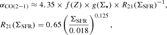 (2)
(2)
and
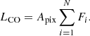 (3)
(3)
Here, Fi denotes the flux of the ith pixel within a cloud, expressed in units of K km s−1, and the total cloud flux was obtained by summing over all pixels belonging to the cloud. Apix is the area of a pixel in pc2. αCO is the CO-to-H2 conversion factor following Schinnerer & Leroy (2024) (see Appendix D for the impact of using another αCO prescription), and LCO is the CO luminosity of the cloud in units of K km s−1 pc2. f(Z) = (Z/Z⊙)−1.5 is the CO-dark factor that depends on the metallicity (Z) for 0.2 < Z/Z⊙ < 2 (see Schinnerer & Leroy 2024 for further information), where Z⊙ is the solar metallicity (12 + log(O/H) = 8.69 as per Asplund et al. 2009). It is worth noting that f(Z) does not take additional factors such as the dust-to-metals ratio, interstellar radiation field, cosmic-ray ionization rate, and the structure of the clouds themselves into consideration, which all play an important role and further add to the uncertainty of the Mmol estimation (see Schinnerer & Leroy 2024). The starburst emissivity factor is g(Σ★) = max(Σ★/100, 1)−0.25, where Σ★ is the stellar mass surface density in units of M⊙ pc−2. Additionally, R21(ΣSFR) is the line ratio of CO(2 − 1) and CO(1 − 0) (see Leroy et al. 2022; Schinnerer & Leroy 2024 for more information). The metallicity was approximated as a function of galactocentric radius based on the global mass-metallicity relation of Sánchez et al. (2019), adopting the PP04 O3N2 calibration (Pettini & Pagel 2004) and extrapolating the predictions to the whole PHANGS-ALMA footprint using a metallicity gradient as per Sánchez et al. (2014) (see Sun et al. 2025).
4. GMC timescales
4.1. The GMC mass function
In the bubble framework of Inutsuka et al. (2015), GMCs form and grow through repeated large-scale compressions of the magnetized ISM (driven by expanding H II regions and supernova shells) while being dispersed by stellar feedback. This picture leads to a continuity equation for the GMC mass function (GMCMF) when neglecting cloud-cloud collisions, as those collisions do not significantly modify the GMCMF evolution, especially in the lower mass range ( ; see Kobayashi et al. 2017),
 (4)
(4)
where ncl(m)≃Ncl/(A × h)/m is the specific volumetric number density of GMCs, Ncl is the number of GMCs within an area (A) of a specific region of the galaxy, h is the molecular scale height of the galactic disk, m is the mass of the GMC, dt is the differential time, and Td is the characteristic self-dispersal timescale (average onset of star formation plus destruction of cloud timescale). The typical star formation-onset timescale (T★) within GMCs was assumed to be ∼10 Myr, as gas in the ISM typically experiences supersonic shocks from supernovae on timescales of ∼1 Myr (e.g., McKee & Ostriker 1977), with the effective interval between shocks (Texp) being shorter due to additional contributions from H II regions. Since only a small fraction of these shocks leads to successful GMC formation (∼3%; see Kobayashi et al. 2017), the characteristic timescale for assembling molecular clouds from the warm neutral medium is Texp/0.03 ∼ 10 Myr. During this successful cloud assembly, these shocks also trigger filamentary structures in clouds, which form massive stars (Inoue et al. 2018; Kumar et al. 2020; Abe et al. 2022; Maity et al. 2024). We therefore adopted T★ = 10 Myr. Additionally, Inutsuka et al. (2015) showed that when running a line-radiation magnetohydrodynamical simulation and including magnetic fields, once a massive star with a mass higher than 30 M⊙ forms, the majority of the mass (> 105 M⊙) of the GMC is destroyed within 4 Myr (see also Hosokawa & Inutsuka 2006; Bonne et al. 2023). Thus, we adopted Td = T★ + 4 = 14 Myr (see Sect. 5.6 for a discussion of how different Td affect the self-growth timescale Tf).
Following Kobayashi et al. (2017), we modeled the mass growth of a GMC as
 (5)
(5)
where Tf(m) is the characteristic self-growth (or formation) timescale for a cloud of mass m. When the mass of the GMC becomes greater than the typical mass of the swept-up shell, the growth of the GMC saturates because the dense gas that can be used to form a cloud becomes limited by the amount of total mass in the expanding shell. A truncation was therefore introduced Tf(m) = Tf [ (1 + m/mtrunc)β], with mtrunc the truncation scale (∼7.7 × 10⁶ M⊙ for a typical Milky Way disk; see the expanding shell argument in Kobayashi et al. 2017) and β = 10 a steepness parameter (see Appendix C for more details). However, for most of the mass range, Tf(m) is nearly constant and equal to a fiducial value Tf. In our analysis, we therefore assumed a constant Tf(m) = Tf and inferred this value from the mass distributions of GMCs (see below). The age to reach mass m by secular growth from a seed mass mmin is then
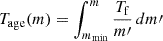 (6)
(6)
that is, exponential mass growth, m(t)∼mminexp(t/Tf).
Following Inutsuka et al. (2015) and Kobayashi et al. (2017), when we combine Eqs. (4) and (5), we obtain
 (7)
(7)
Solving this form of the GMCMF with a steady-state assumption (∂ncl/∂t = 0) yields a steady-state solution
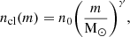 (8)
(8)
where
 (9)
(9)
 (10)
(10)
Here, γ is the power-law index, and n0 is the differential number density normalized at m = 1 M⊙. Equation (10) implies that the slope of the GMCMF provides information about the timescale of GMCs (see Sect. 5.1). We adopted Td = 14 Myr, as previously explained, and we estimated Tf from γ.
The γ index can be measured from the GMC mass spectra given by the following equation:
![Mathematical equation: $$ \begin{aligned} \frac{dN}{dM} \propto M^{\gamma } \implies N(M\prime > M) = N_{0} \bigg [\bigg (\frac{M}{M_{0}}\bigg )^{\gamma +1} - 1\bigg ]. \end{aligned} $$](/articles/aa/full_html/2026/06/aa59653-26/aa59653-26-eq15.gif) (11)
(11)
Equation (11) refers to the solution of the integral of the GMCMF, which yields the cumulative mass spectrum. The slope of the mass spectra can be used to infer the γ parameter. We followed a truncated power law for our functional form (see also Williams & McKee 1997; Colombo et al. 2014). The maximum mass of the distribution is presented by M0, and N0 refers to the number of clouds with masses higher than 21/(γ + 1)M0 (i.e., the truncation mass where the distribution deviates from a single power law).
As a practical choice, we adopted mmin = 104 M⊙ for the minimum GMC mass or completeness limit and estimatde Tf following Eq. (10) globally in each galaxy and per galactic environment (see Appendix B for the effect of changing the completeness limit). The completeness limit set here refers to a limit where less massive clouds may not host massive stars as frequently as more massive clouds (see B26 on the minimum contribution of clouds less massive than 104 M⊙ to star formation) and have less self-destruction by feedback from these stars. Then, we estimated the individual cloud formation timescale following Eq. (6). In Appendix D, we show the effect of changing the αCO factor on our analysis.
4.2. Other timescales
In addition to the basic framework introduced above, this section provides all the different time estimates we calculated for each cloud. The measurements are compiled in Table A.1 for each galaxy.
-
Free-fall timescale (Tff):
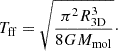 (12)
(12)This timescale describes the time required for a cloud to collapse in free fall due to the gravity of the cloud, provided that no pressure supports the system. Here, R3D is the three-dimensional radius of the cloud, estimated as
![Mathematical equation: $ R_{\mathrm{3D}} = \min{\bigg[R_{\mathrm{eq}}, \bigg(R_{\mathrm{eq}}^{2} \sqrt{\frac{h}{2\cos{i}}}\bigg)^{1/3}\bigg]} $](/articles/aa/full_html/2026/06/aa59653-26/aa59653-26-eq17.gif) , and Req is the equivalent radius of the cloud calculated from the number of pixels within the cloud (
, and Req is the equivalent radius of the cloud calculated from the number of pixels within the cloud ( , where Acloud is the area of the cloud, and it was directly estimated from the number of pixels within the cloud multiplied by the area of the pixel in pc2). The molecular gas disk scale height h was assumed to be 100 pc (Heyer & Dame 2015), and
  would be the inclination-corrected molecular disk scale height.
 -
Orbital time (Torb):
 (13)
(13)This is the period of the orbital revolution around the center of a galaxy. To approximate the angular velocity Ωcirc, we used rotation curve measurements from Sun et al. (2022) that were derived from CO line kinematics to find Ωcirc. The measurements were based on the PHANGS-ALMA dataset (Leroy et al. 2021) and were performed in radial bin sizes of 150 pc. We specifically adopted the universal rotation curve functional form suggested by Persic et al. (1996) for the rotation curves. Based on these best-fit analytical models of the co-rotation curves and the estimated uncertainties on the model parameters, the circular velocity (Vcirc), Ωcirc, and the logarithmic derivative of the rotation curve
 (where Rgal is the galactocentric distance) was extrapolated at each radius (see Sun et al. 2022 for more information). Orbital timescales for the clouds were estimated for 60 galaxies for which the rotation curve was measured.
 -
Shearing time (Tshear):
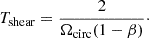 (14)
(14)Following Sun et al. (2022), this is the timescale for two objects to move closer/farther by a unit length azimuthally, given that they are on two circular orbits separated radially by the same unit length. The shearing timescale was estimated for clouds in 60 galaxies for which the rotation curve was measured.
-
Depletion time (Tdep):
 (15)
(15)This timescale corresponds to the inverse of the star formation efficiency (SFE). It indicates how long it would take a cloud to deplete its molecular gas reservoir at its current SFR. The depletion time was calculated for clouds in the 19 PHANGS-JWST Cycle 1 galaxies.
5. Results and discussion
In this section, we present the parameters of the truncated power-law fit. We then compare the GMC timescale estimates per galaxy and galactic environment, and to other timescale estimate methods. We used the PHANGS simple galactic environment masks (Querejeta et al. 2021), which classify regions into center (bulge or nucleus), bar (including bar ends), spiral arm, inter-arm, and disk (outside the bar) in galaxies lacking spiral arms (for more details, see B26). We also investigated whether there was a dependence of Tf and galactocentric radius, which might indicate large-scale processes that affect the evolution of GMCs (e.g., shear or gravity). Additionally, Table A.1 presents the timescale measurements in each galaxy.
5.1. The power-law index
The mass spectra of GMCs provide a straightforward way to understand the relative differences between regions within and across galaxies, as well as an intuitive understanding of whether most of the mass resides in low- or high-mass clouds. Specifically, the slope of the mass spectra would reflect which population of clouds dominates the mass distribution, with shallower slopes indicating the prominence of more massive clouds (e.g., Colombo et al. 2014; Faustino Vieira et al. 2024). A traditional way of fitting the mass spectra is by either a single power or a truncated power law (e.g., Williams & McKee 1997), since the mass spectrum generally steepens at high cloud masses (e.g., Fukui et al. 2001; Rosolowsky 2007). The functional form of this truncated power law is presented in Eq. (11), where the γ + 1 power-law index reflects the slope. The γ parameter is also the slope of the GMCMF, which means that the prominence of low- or high-mass clouds would give us information about the evolutionary track of GMCs within a galaxy, and it might be used to trace the lifetime of GMCs (e.g., Inutsuka et al. 2015; Kobayashi et al. 2017).
We therefore fit a truncated power law on the mass spectra across 66 galaxies and their different galactic environments. For the fits, we applied 100 bootstrap resamples while including the error on Mmol. The fit parameters are presented in Table 1. An example of the truncated power-law fit on NGC 0628 is displayed in Fig. 1. We used a Python-based fitting procedure similar to the approach used in Rosolowsky (2005)2. The γ parameter varied by up to a factor of two across galaxies, environments, and within the same environment across galaxies. This is also reflected in the log-normal distribution fit in B26, which indicates that the galactic environment and the galactic conditions both play a role in driving different mass distributions (the different factors are discussed in Sects. 5.2, 5.3, and 5.4). Generally, the shallowest slope is found for clouds within the central regions of the galaxies, followed by disks and spiral arms. This implies that those environments host more contribution from massive clouds to their mass spectrum compared to the inter-arm and bar regions. However, a caveat applies to the central regions, where overlapping GMCs cannot be distinguished in two-dimensional images, which might lead to artificially shallower slopes. Additionally, individual galaxies might show variation in their trend (see Table A.1).
 |
Fig. 1. Example of the truncated power-law fit on NGC 0628. We present the fit on all clouds (global) and per galactic environment (center, S-arm, and I-arm). The vertical dashed line shows the completeness limit we set in our analysis. The dashed curve shows the truncated power-law fit. The fit parameters are presented in the box in the lower left region of each plot. |
Parameters of the truncated power-law fit of the GMC mass spectrum across the galaxies.
Table 2 shows the Spearman correlation between γ and global galactic properties and cloud properties. The strongest correlations are with cloud-scale molecular mass surface density (Σmol) and the star formation rate surface density (ΣSFR), highlighting the role of localized processes, such as shocks from massive stars and supernovae, in enhancing cloud formation (see Sect. 5.2 for more information). The most notable anticorrelations are with M★ and SFR. This suggests that global star formation activity and galactic potential within galaxies drive steeper slopes in the mass spectrum, possibly due to the destruction of massive GMCs by feedback processes. On the other hand, the correlation between γ and Mmol implies that more molecular gas in galaxies leads to more massive GMCs.
Spearman correlation coefficients (ρ) and p values between the GMC mass function slope γ and selected galactic/cloud properties across the 66 galaxies, ordered by decreasing |ρ|.
5.2. Cloud formation drivers within galaxies
In this section, we examine the factors that may affect the various cloud formation timescales within galaxies. To do this, we tested whether star formation and the gas surface densities might play a role in enhancing their formation.
In the left panel of Fig. 2, we binned GMCs in each galaxy into five separate bins (quantiles; Q1–Q5) of increasing cloud-level Σmol, and within each galaxy, each bin had the same number of GMCs. We then computed γ and Tf from the mass spectra in each of the bins to test whether regions with high Σmol form clouds more quickly. The most notable difference is between the highest Σmol quantile and the lowest one, with a GMC formation quicker by 6.8 ± 2.2 Myr on average for the highest Σmol. The highest difference between Q5 and Q1 is measured for NGC 4321 (barred spiral galaxy) with ∼12.1 ± 2.8 Myr, followed by NGC 1566 (barred spiral galaxy) with 9.4 ± 2.4 Myr, and NGC 4254 (spiral galaxy) with ∼9.1 ± 2.4 Myr. Generally, in ∼73% of the barred galaxies, the formation in the highest Σmol quantile is significantly faster than in the lowest quantile. This might also indicate that a bar might play an additional role in accelerating cloud formation through large-scale gas inflows, for instance.
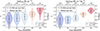 |
Fig. 2. Violin plots showing the distribution of the GMC mass spectra slope γ and Tf in increasing (Q1 to Q5) cloud-scale Σmol (left) and ΣSFR (right) bins within 66 (PHANGS Cycle 1 and 2) and 19 (PHANGS Cycle 1) galaxies, respectively. The upper x-axis shows the property median of each bin across the galaxies, with quantiles corresponding to the |


We also binned the galaxies into five separate bins of increasing cloud-level ΣSFR in the right panel of Fig. 2. This helped us to assess whether local star formation activity, which regulates the frequency of shocks from massive stars and supernovae, has a measurable effect on the cloud lifetimes. The most notable difference between the quantiles is Q5 and Q1 (∼6.9 ± 1.9 Myr) on average, specifically, in NGC 4321 (barred spiral) with ∼12.0 ± 1.9 Myr, in NGC 0628 (spiral galaxy) with ∼11.3 ± 2.2 Myr, and in NGC 1087 (barred disk) with ∼8.1 ± 2.1 Myr. This indicates that star formation might drive a faster cloud formation through supersonic compression of the surrounding gas (Kobayashi et al. 2017). Moreover, the highest contrast between the Σmol and ΣSFR bins is within spiral galaxies (∼77% of spirals), which indicates that spiral arms might play an additional role in enhancing cloud formation through spiral density waves, high Σmol regions, and additional supersonic compressions.
We estimated the exponential growth time Tage(m) of individual clouds assuming that clouds reach their mass m by secular growth from a seed mass mmin = 104 M⊙ using Eq. (6). In Fig. 3, the average age of individual clouds increases with SFR and M★. Kim et al. (2022) (see also Pan et al. 2022) reported similar trends, although they excluded galactic centers when estimating the cloud lifetime using a CO- and Hα-based analysis using the prescription of Kruijssen & Longmore (2014). This increase is expected, since the correlation between the molecular mass of the cloud and Tage(m) is exponential, according to Eq. (6). This implies that more massive clouds take longer to form than smaller clouds. Because SFR and M★ are also correlated since more star-forming galaxies tend to be more massive, an increase of Tage(m) with SFR is expected.
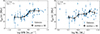 |
Fig. 3. Scatter plots with error bars showing the variation in the median Tage(m) with log SFR (left) and log M★ (right) for the 66 galaxies in our sample. The black line shows the running median with the same number of galaxies in each bin, and the error is the standard error on the median. The Spearman correlation coefficient (ρ) is presented in each figure with the p value. Galaxies tend to have a longer cloud formation time with increasing SFR and M★. |
We further split galaxies into active (hosting an AGN) and inactive following Véron-Cetty & Véron (2010). Out of the galaxies in the sample, 15 are classified as active. The formation timescale is similar across galactic environments between the groups. Therefore, the effect of instantaneous AGN feedback in our sample may be minimal and does not significantly reflect or affect the formation of GMCs.
5.3. Cloud formation across galactic environments
As mentioned before, the dispersal time for each cloud was assumed to be mainly driven by stellar radiative feedback and was assumed to be constant (see Sect. 5.6 for further discussion). We estimated the exponential growth time of individual clouds using Eq. (6). In Fig. 4 and Table 3, we provide median measurements for the 66 galaxies in our sample. However, it is worth noting that the central regions contain reasonably higher star and dust continuum than the other environments. So there exists a caveat toward central regions, and the timescale values might be slightly higher when we subtract these contaminants.
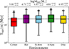 |
Fig. 4. Bar plot with outliers (in circles) showing the exponential growth timescale, Tage(m), of GMCs across the galactic environment in 66 galaxies. The upper x-axis shows the median cloud Mmol with a 84th–50th and 50th–16th percentile distribution as upper and lower limits, respectively. The dashed black line represents the median timescale for all the clouds. On average, clouds with Mmol ≤ 105 M⊙ form in ≲20 Myr, with more massive clouds (106 − 7 M⊙) taking up to 100 Myr. Also, central clouds form the quickest compared to other environments by ∼0.3 dex. |
Median GMC formation timescales and ages by galactic environment across the galaxies.
In general, the central regions exhibit the lowest Tage(m) compared to other galactic environments across the galaxies by ∼10 − 15 Myr on average. Their extreme environments, high Σmol, and high ΣSFR allow them to form clouds faster. Bars and inter-arm GMCs have ∼2 ± 1 Myr longer Tage(m) on average than spiral arm and disk GMCs. The low Tage(m) in bar GMCs is mainly driven by low Σmol and ΣSFR regions in dusty lanes, where the population of GMCs tends to be dominated by lower masses compared to other environments (see also B26).
Generally, in ∼58% of the spiral galaxies, spiral arms form GMC faster than inter-arm regions. Notably, NGC 3627, NGC 2090, and NGC 1672 show a cloud formation that is quicker by 9.7 ± 2.1, 7.5 ± 1.4, and 6.6 ± 1.6 Myr, respectively, in their spiral arms compared to inter-arm regions, which is mainly driven by higher Σmol, and ΣSFR in the arms (see Querejeta et al. 2024 and B26). As highlighted in Sect. 5.2, supersonic compressions and density waves within the spiral arms might play a role in quickening the cloud formation in arm regions.
5.4. Cloud formation across galactocentric radius
Examination of Tage(m) as a function of galactocentric radius (Rgal) provides insight into whether the average cloud formation timescale varies systematically across galaxy disks. Processes such as gravitational torques, spiral density waves, and hydrodynamic shocks (e.g., Lin & Shu 1964; Roberts et al. 1979; Sormani & Barnes 2019; Yu et al. 2022) primarily act on scales larger than individual clouds, shaping the spatial arrangement and surface density of the molecular gas and driving radial gas redistribution over timescales longer than typical cloud lifetimes. By contrast, cloud formation itself may proceed through local and transient instabilities, such as the Parker instability (e.g., Parker 1966) and swing amplification (e.g., Goldreich & Lynden-Bell 1965; Julian & Toomre 1966; Toomre 1981; Fuchs 2001; Binney 2020). The latter drives density waves, which then rapidly compress gas and form clouds on timescales comparable to the free-fall time (e.g., Meidt & van der Wel 2024). Trends with Rgal are therefore generally not intended to isolate the effect of specific dynamical structures such as bars or spiral arms, which are more appropriately probed through azimuthal variations or within the galactic environment, but rather to assess whether the average cloud formation timescale exhibits a systematic radial behavior.
Figure 5 shows the variation of Tage(m) as a function of Rgal for all 66 galaxies. The global trend across the galaxies shows ∼0.1 dex lower Tage(m) on average in the central 0.3 stellar effective radius than in the outer regions. We then split grand-design spirals, and the rest were multi-armed, flocculent spirals or disk (lacking spiral features) galaxies following Querejeta et al. (2024), where galaxies were visually classified from near-infrared imaging following Buta et al. (2015) classification scheme for galaxies in the S4G survey. On average, Tage(m) shows no significant difference between the different galaxy groups at different Rgal, indicating that cloud formation is largely alike in spiral and disk galaxies with similar average cloud Σmol values (see B26).
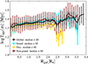 |
Fig. 5. Growth time of the clouds, Tage(m), as a function of galactocentric radius for the sample of 66 galaxies split into grand-design spirals (prominent spiral features), non-grand-design spirals, and disk galaxies (no spiral features). The binned median per galaxy group is shown as solid lines, with error bars representing the standard error on the median (SE = |

Most galaxies also exhibit flat trends in Tage(m) across all Rgal. Some exceptions are galaxies hosting central molecular zones (CMZs), such as NGC 1365, NGC 1433, and NGC 3627. These galaxies have timescales that are shorter by 0.2−1 dex toward their CMZs than in the outer regions, indicating an additional role of the extreme environment in the CMZ in driving a quicker cloud formation.
Figure 6 shows that cloud formation timescales in spiral arm regions are slightly shorter on average than in inter-arm regions, with typical offsets of ∼0.1 dex. However, these differences are modest and comparable to the intrinsic scatter at fixed Rgal. The small systematic offset suggests that spiral arms may provide enhancement to cloud formation, potentially through increased gas surface density and orbit crowding, and do not drive a fundamentally distinct formation mode. Clouds in the galactic disk environment appear to have similar timescales to those of spiral arms in the outer regions. However, toward the inner 0.3 Re, spiral arms show a could formation that is quicker by ∼0.2 dex than in disks. This might highlight the role of large-scale inflows via arms and bars. Within bars, however, and specifically, in bar lanes, the cloud Σmol is relatively lower than in other environments (see B26), which might prevent the formation of massive GMCs. It is also worth noting that within PHANGS galaxies, spiral arms have a 0.1 − 0.2 dex higher Σ★, a 0.2 − 0.5 dex higher Σmol, and a 0.2 − 0.5 dex higher ΣSFR on average compared to inter-arm regions (see Querejeta et al. 2024 and B26).
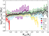 |
Fig. 6. Growth time of the clouds, Tage(m), as a function of galactocentric radius for the sample of 66 galaxies split according to galactic environment. The binned median per galaxy group is shown as solid lines, with error bars representing the standard error on the median. The solid black line represents the median trend for all the clouds regardless of galaxy group. All trends seem to be consistent with each other, with a ∼0.2 dex drop in the central regions. The scatterplot is a 2D histogram for the whole sample. |
5.5. The different timescales of clouds
Figure 7 shows the distribution of Tage(m) with respect to all other timescales for the galaxies in our sample. The timescales we present refer to those that take place within the cloud (Tdep, and Tff) and to those that occur on larger scales up to the scale of the galaxy (Tshear and Torb). Tdep is ∼1 − 5 Gyr in our sample, which is consistent with other studies on molecular-gas-dominated regions in nearby massive star-forming galaxies (e.g., Bigiel et al. 2008; Ellison et al. 2021; Sun et al. 2022). Tff operates on timescales of ∼5 − 20 Myr. These two timescales mean that the efficiency of the star formation per free-fall time is ∼0.1%−2%. This reaffirms that star formation is inefficient in nearby star-forming galaxies (see also Evans et al. 2014; Utomo et al. 2017; Sun et al. 2022). When we assume that clouds take ∼1 − 5 Myr to disperse from stellar feedback (e.g., Inutsuka et al. 2015; Kim et al. 2022; Bonne et al. 2023) and that the formation of individual clouds operates on timescales of tens of million years (as depicted in Table 3), the depletion per cloud lifetime is ∼1%, which is consistent with previous studies (e.g., Kruijssen et al. 2019; Chevance et al. 2020a; Kim et al. 2021). This further highlights the inefficiency of the star formation.
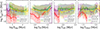 |
Fig. 7. Growth timescale as a function of Tdep (Eq. 15), Tff (Eq. 12), Torb (Eq. 13), and Tshear (Eq. 14). The median trend is plotted across galactic environments for the galaxies in our sample. The shaded region represents the 84th–50th, and 50th–16th percentiles, and the error bar is the standard error on the median. The Spearman correlation coefficient ρ is written in black when the correlation is significant (p < 0.05). Otherwise, it is not significant. |
The timescales that are associated with dynamical processes acting on kiloparsec scales (e.g., Tshear and Torb) take place over ∼60 − 200 Myr. The order-of-magnitude contrast between them and Tff implies that the effects of galactic-scale dynamics on individual molecular clouds are minimal. The shearing time being ∼0.6 dex higher than Tff indicates that shearing motions are generally small on cloud scales relative to motions generated by gravitational collapse (see also Sun et al. 2022), and Torb being ∼0.8 dex higher than Tage(m) indicates that molecular clouds can only last a small fraction of a complete orbital revolution around the galaxy center (e.g., Chevance et al. 2020a,b).
We also examined the correlation between Tage(m) and the other timescales using Spearman ρ (correlation) and p (probability) values. Among all comparisons, Tage(m) does not correlate with any of the timescales, as shown in Fig. 7. However, a typical offset of ∼0.1 dex between Tage(m) and Tff, with Tage(m) > Tff, indicates that the cloud lifetimes exceed the timescale required for gravitational collapse. This implies that additional physical processes, such as stellar feedback, act to slow collapse and prolong cloud evolution beyond a single free-fall time.
5.6. Cloud destruction across galaxies
In the previous sections, we assumed a star-formation-onset timescale within GMCs of 10 Myr (T★ = 10 Myr; see Sect. 4) and a destruction time of 4 Myr after the onset. Therefore, the self-dispersal timescale Td was set to be T* + 4 = 14 Myr. The underlying oversimplified assumption of a constant cloud-destruction time is that the SFE is universal for the population-average cloud properties across a mass spectrum (see Inutsuka et al. 2015). However, cloud destruction might not be universal (e.g., Federrath & Klessen 2012; Wainer et al. 2026), and recent studies showed that the feedback time within clouds can vary from 1 − 5 Myr, with an average of ∼4 Myr (see Chevance et al. 2020b; Kim et al. 2021, 2022; Ramambason et al. 2026). Therefore, in this section, we test the variation in Tf when the prescription for Td is changed.
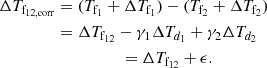
Figure E.1 shows that upon varying Td between 10 + 1 Myr and 10 + 5 Myr (the destruction timescale varies between 1 − 5 Myr across galaxies; see Kim et al. 2022), the formation time increases by a factor of γ. Steeper slopes imply longer Tf values. On the other hand, shallower slopes imply a faster cloud formation. However, when stellar feedback drives cloud destruction at longer timescales, the average formation time of clouds within galaxies would be affected by an additional ΔTf = −(γ + 1)×ΔTd according to the GMCMF prescription. Thus, the corrected difference of a varying Td from comparing different formation timescales across two different mass spectra, which is depicted as the shaded region in Fig. E.1, would be
 (16)
(16)
Here, both indices γ1 and γ2 are constants per galaxy. However, the variables are ΔTd1 and ΔTd2. If Td is universal, then ΔTf12, corr will be equal to ΔTf12. The power-law index γ might vary between −1.2 and −2.0, and Td might vary between 1 and 5 Myr. If Td is accurately calculated, with a variable SFE prescription, then the SFE-dependent factor (ϵ = −γ1ΔTd1 + γ2ΔTd2) would be introduced.
It is worth noting that if ϵ changes, it creates more contrast between the galactic environments. Multiple scenarios are envisioned if ϵ changes, some of which are that low Σmol clouds might be destroyed faster than high Σmol clouds, thus leading to similar Tf values between inter-arm and spiral arm regions. High Σmol clouds might be destroyed faster than low Σmol clouds, thus leading to more contrast in Tf between arms and inter-arms. However, our Tage(m) values, given a constant Td, are within the range of estimates from previous works (e.g., Chevance et al. 2020a; Kim et al. 2022, 2025).
6. Summary and conclusions
We used PAH-based GMCs identified from stellar-continuum-subtracted JWST/F770W maps, combined with PHANGS-ALMA CO(2−1) measurements and ancillary galaxy properties, to characterize the secular growth and evolutionary timescales of molecular clouds in 66 nearby star-forming galaxies. The cloud formation was interpreted within the steady-state cloud mass function framework of Inutsuka et al. (2015) and Kobayashi et al. (2017), who considered that GMCs form and grow through multiple repeated stellar feedback compressions. This model links the GMC mass function slope to a characteristic self-growth timescale Tf and a mass-dependent secular age Tage(m) (Eq. 6). We also assumed a constant GMC self-dispersal timescale of 14 Myr in our analysis. Below, we summarize our main findings.
-
The slope γ of the GMC mass spectra varies across different environments: The values of γ are generally between −1.2 and −2.0. The centers have the shallowest slopes and the highest maximum masses, followed by spiral arms and disks. This and the positive correlation of γ with Mmol indicate that massive clouds dominate the mass distribution in these environments compared to bars and inter-arms.
-
The average ages of clouds vary according to secular growth Tage(m): Clouds with masses ≤105 M⊙ form in ∼20 Myr, while more massive clouds (106 − 7 M⊙) take up to 100 Myr.
-
The cloud formation varies systematically across galaxies: Cloud growth proceeds fastest in systems with higher molecular gas surface densities and more massive GMC populations, indicating that dense gas-rich conditions favor an efficient secular cloud assembly.
-
High-Σmol and -ΣSFR regions accelerate cloud growth: Within individual galaxies, clouds in regions of high-Σmol or -ΣSFR display shorter Tf than those in low-Σmol or -ΣSFR environments. The contrast can reach several million years in barred actively star-forming systems. This suggests that the gas density, stellar feedback, dynamical compression, or all together might promote faster GMC growth.
-
The environmental dependence of Tage(m). Median cloud ages differ substantially between galactic environments: Central regions show the shortest Tage(m) (typically ∼16 Myr), ∼5 − 10 Myr lower than in spiral arms, inter-arms, or disks. Inter-arm and bar environments show the longest Tage(m), which is mainly driven by low Σmol within the disk and bar lanes.
-
The radial gradients reflect the effect of central molecular zones: Throughout the full sample, Tage(m) decreases toward small galactocentric radii, with a typical drop of ∼0.1 − 0.2 dex inside ∼0.3 Re. Galaxies hosting a bright dense central molecular zone exhibit the strongest gradients, with central clouds forming up to ∼0.2 − 1.0 dex faster than those in their outer disks. In contrast, galaxies lacking prominent non-axisymmetric structure show nearly flat radial trends.
-
The hierarchy of internal and galactic dynamical timescales: The GMC depletion time operates at scales of billions of years, while the free-fall times are ∼5 − 20 Myr. The shear and orbital times are much longer (∼60 − 200 Myr). The strong contrast between these quantities demonstrates that GMC evolution unfolds on timescales much shorter than those associated with galactic rotation or shear. However, shearing processes such as swing-amplification might still play a role in cloud formation.
-
Cloud growth and free-fall time: Tage(m) is higher by ∼0.1 dex on average than Tff (see Fig. 7), which indicates that clouds might persist for several free-fall times, requiring the presence of non-gravitational support such as turbulence, magnetic fields, or stellar feedback.
-
Implications for GMC life cycles and star formation efficiency: When we combine Tage(m), Tff, and plausible dispersal times due to feedback (a few million years), GMCs are expected to convert only ∼1% of their gas into stars over their lifetime. This is consistent with a picture in which cloud assembly, collapse, and destruction are jointly regulated by self-gravity, feedback, and large-scale galactic flows, leading to inherently inefficient star formation in nearby disk galaxies.
In summary, we found cloud lifetimes that are consistent on average with previous efforts that used cloud identification methods (Blitz et al. 2007; Fukui et al. 2008; Meidt et al. 2015; Corbelli et al. 2017), statistics of sight-line fractions with only CO or only Hα or both types of emission (Schinnerer et al. 2019; Pan et al. 2022), and those that used the tuning-fork analysis (Kruijssen et al. 2019; Chevance et al. 2020b; Kim et al. 2021, 2022, 2025). Future work would include a more focused analysis to determine the destruction timescale of clouds. Because this timescale varies per galaxy (e.g., Kim et al. 2022) and might also vary within each galaxy, a prescription of Td that takes this into account would be beneficial for our understanding of the mass distribution in galaxies.
Acknowledgments
This work has been carried out as part of the PHANGS collaboration. This work is based on observations made with the NASA/ESA/CSA JWST. The data were obtained from the Mikulski Archive for Space Telescopes at the Space Telescope Science Institute, which is operated by the Association of Universities for Research in Astronomy, Inc., under NASA contract NAS 5-03127 for JWST. These observations are associated with programs 2107 and 3707. ZB, DC, and FB gratefully acknowledge the Collaborative Research Center 1601 (SFB 1601 sub-project B3) funded by the Deutsche Forschungsgemeinschaft (DFG, German Research Foundation) – 500700252. M.I.N.K. is supported by Grants-in-Aid from the Ministry of Education, Culture, Sports, Science, and Technology of Japan (JP22K14080). S.K.S. is supported by an International Research Fellowship of the Japan Society for the Promotion of Science (JSPS). MB acknowledges support from the ANID BASAL project FB210003. This work was supported by the French government through the France 2030 investment plan managed by the National Research Agency (ANR), as part of the Initiative of Excellence of Université Côte d’Azur under reference number ANR-15-IDEX-01. HAP acknowledges support from the National Science and Technology Council of Taiwan under grant 113-2112-M-032-014-MY3. LECR is supported by the Deutsche Forschungsgemeinschaft (DFG, German Research Foundation) under Germany’s Excellence Strategy – EXC 2094/2 – 390783311. MQ and MJJD acknowledge support from the Spanish grant PID2022-138560NB-I00, funded by MCIN/AEI/10.13039/501100011033/FEDER, EU. RSK acknowledges financial support from the ERC via Synergy Grant “ECOGAL” (project ID 855130) and from the German Excellence Strategy via the Heidelberg Cluster “STRUCTURES” (EXC 2181 – 390900948). In addition RSK is grateful for funding from the German Ministry for Economic Affairs and Climate Action in project “MAINN” (funding ID 50OO2206), and from DFG and ANR for project “STARCLUSTERS” (funding ID KL 1358/22-1). AR and LR gratefully acknowledge funding from the DFG through an Emmy Noether Research Group (grant number CH2137/1-1).
References
- Abe, D., Inoue, T., Enokiya, R., & Fukui, Y. 2022, ApJ, 940, 106 [Google Scholar]
- Ali, A., Harries, T. J., & Douglas, T. A. 2018, MNRAS, 477, 5422 [NASA ADS] [CrossRef] [Google Scholar]
- Asplund, M., Grevesse, N., Sauval, A. J., & Scott, P. 2009, ARA&A, 47, 481 [NASA ADS] [CrossRef] [Google Scholar]
- Barnes, A. T., Watkins, E. J., Meidt, S. E., et al. 2023, ApJ, 944, L22 [NASA ADS] [CrossRef] [Google Scholar]
- Bazzi, Z., Colombo, D., Bigiel, F., et al. 2026, A&A, 706, A40 [NASA ADS] [CrossRef] [EDP Sciences] [Google Scholar]
- Belfiore, F., Leroy, A. K., Sun, J., et al. 2023, A&A, 670, A67 [NASA ADS] [CrossRef] [EDP Sciences] [Google Scholar]
- Bigiel, F., Leroy, A., Walter, F., et al. 2008, AJ, 136, 2846 [NASA ADS] [CrossRef] [Google Scholar]
- Binney, J. 2020, MNRAS, 496, 767 [NASA ADS] [CrossRef] [Google Scholar]
- Blitz, L., Fukui, Y., Kawamura, A., et al. 2007, in Protostars and Planets V, eds. B. Reipurth, D. Jewitt, & K. Keil, 81 [Google Scholar]
- Bolatto, A. D., Wolfire, M., & Leroy, A. K. 2013, ARA&A, 51, 207 [CrossRef] [Google Scholar]
- Bonne, L., Kabanovic, S., Schneider, N., et al. 2023, A&A, 679, L5 [NASA ADS] [CrossRef] [EDP Sciences] [Google Scholar]
- Brucy, N., Vázquez-Semadeni, E., Colman, T., Fensch, J., & Klessen, R. S. 2025, Open J. Astrophys., 8, 54637 [Google Scholar]
- Buta, R. J., Sheth, K., Athanassoula, E., et al. 2015, ApJS, 217, 32 [Google Scholar]
- Chevance, M., Kruijssen, J. M. D., Hygate, A. P. S., et al. 2020a, MNRAS, 493, 2872 [NASA ADS] [CrossRef] [Google Scholar]
- Chevance, M., Kruijssen, J. M. D., Vazquez-Semadeni, E., et al. 2020b, Space Sci. Rev., 216, A50 [Google Scholar]
- Chown, R., Li, C., Parker, L., et al. 2020, MNRAS, 500, 1261 [NASA ADS] [CrossRef] [Google Scholar]
- Chown, R., Leroy, A. K., Sandstrom, K., et al. 2025, ApJ, 983, 64 [Google Scholar]
- Colombo, D., Hughes, A., Schinnerer, E., et al. 2014, ApJ, 784, 3 [NASA ADS] [CrossRef] [Google Scholar]
- Colombo, D., Rosolowsky, E., Ginsburg, A., Duarte-Cabral, A., & Hughes, A. 2015, MNRAS, 454, 2067 [NASA ADS] [CrossRef] [Google Scholar]
- Congiu, E., Blanc, G. A., Belfiore, F., et al. 2023, A&A, 672, A148 [NASA ADS] [CrossRef] [EDP Sciences] [Google Scholar]
- Corbelli, E., Braine, J., Bandiera, R., et al. 2017, A&A, 601, A146 [NASA ADS] [CrossRef] [EDP Sciences] [Google Scholar]
- Dale, J. E. 2015, New Astron. Rev., 68, 1 [CrossRef] [Google Scholar]
- Dale, D. A., Graham, G. B., Barnes, A. T., et al. 2025, AJ, 169, 133 [Google Scholar]
- den Brok, J. S., Cantalupo, S., Mackenzie, R., et al. 2020, MNRAS, 495, 1874 [Google Scholar]
- Draine, B. T., & Li, A. 2007, ApJ, 657, 810 [CrossRef] [Google Scholar]
- Ellison, S. L., Lin, L., Thorp, M. D., et al. 2021, MNRAS, 501, 4777 [NASA ADS] [CrossRef] [Google Scholar]
- Emsellem, E., Schinnerer, E., Santoro, F., et al. 2022, A&A, 659, A191 [NASA ADS] [CrossRef] [EDP Sciences] [Google Scholar]
- Evans, N. J., II, Heiderman, A., & Vutisalchavakul, N. 2014, ApJ, 782, 114 [CrossRef] [Google Scholar]
- Faustino Vieira, H., Duarte-Cabral, A., Davis, T. A., et al. 2024, MNRAS, 527, 3639 [Google Scholar]
- Federrath, C., & Klessen, R. S. 2012, ApJ, 761, 156 [Google Scholar]
- Field, G. B., Goldsmith, D. W., & Habing, H. J. 1969, ApJ, 155, L149 [NASA ADS] [CrossRef] [Google Scholar]
- Fuchs, B. 2001, A&A, 368, 107 [NASA ADS] [CrossRef] [EDP Sciences] [Google Scholar]
- Fukui, Y., & Kawamura, A. 2010, ARA&A, 48, 547 [NASA ADS] [CrossRef] [Google Scholar]
- Fukui, Y., Mizuno, N., Yamaguchi, R., Mizuno, A., & Onishi, T. 2001, PASJ, 53, L41 [Google Scholar]
- Fukui, Y., Kawamura, A., Minamidani, T., et al. 2008, ApJS, 178, 56 [Google Scholar]
- Fukushima, H., & Yajima, H. 2021, MNRAS, 506, 5512 [NASA ADS] [CrossRef] [Google Scholar]
- Gao, Y., Xiao, T., Li, C., et al. 2019, ApJ, 887, 172 [Google Scholar]
- Geen, S., Soler, J. D., & Hennebelle, P. 2017, MNRAS, 471, 4844 [NASA ADS] [CrossRef] [Google Scholar]
- Goldreich, P., & Lynden-Bell, D. 1965, MNRAS, 130, 125 [Google Scholar]
- Heyer, M., & Dame, T. M. 2015, ARA&A, 53, 583 [Google Scholar]
- Hollenbach, D. J., & Tielens, A. G. G. M. 1999, Rev. Mod. Phys., 71, 173 [Google Scholar]
- Hosokawa, T., & Inutsuka, S.-I. 2006, ApJ, 646, 240 [NASA ADS] [CrossRef] [Google Scholar]
- Inoue, T., & Inutsuka, S.-I. 2008, ApJ, 687, 303 [NASA ADS] [CrossRef] [Google Scholar]
- Inoue, T., & Inutsuka, S.-I. 2009, ApJ, 704, 161 [NASA ADS] [CrossRef] [Google Scholar]
- Inoue, T., & Inutsuka, S.-I. 2012, ApJ, 759, 35 [Google Scholar]
- Inoue, T., Hennebelle, P., Fukui, Y., et al. 2018, PASJ, 70, S53 [NASA ADS] [Google Scholar]
- Inutsuka, S.-I., Inoue, T., Iwasaki, K., & Hosokawa, T. 2015, A&A, 580, A49 [NASA ADS] [CrossRef] [EDP Sciences] [Google Scholar]
- Iwasaki, K., Tomida, K., Inoue, T., & Inutsuka, S.-I. 2019, ApJ, 873, 6 [NASA ADS] [CrossRef] [Google Scholar]
- Julian, W. H., & Toomre, A. 1966, ApJ, 146, 810 [NASA ADS] [CrossRef] [Google Scholar]
- Kawamura, A., Mizuno, Y., Minamidani, T., et al. 2009, ApJS, 184, 1 [NASA ADS] [CrossRef] [Google Scholar]
- Kim, C.-G., & Ostriker, E. C. 2017, ApJ, 846, 133 [NASA ADS] [CrossRef] [Google Scholar]
- Kim, J.-G., Kim, W.-T., Ostriker, E. C., & Skinner, M. A. 2017, ApJ, 851, 93 [NASA ADS] [CrossRef] [Google Scholar]
- Kim, J., Chevance, M., Kruijssen, J. M. D., et al. 2021, MNRAS, 504, 487 [NASA ADS] [CrossRef] [Google Scholar]
- Kim, J., Chevance, M., Kruijssen, J. M. D., et al. 2022, MNRAS, 516, 3006 [NASA ADS] [CrossRef] [Google Scholar]
- Kim, J., Chevance, M., Ramambason, L., et al. 2025, ApJ, 988, 215 [Google Scholar]
- Klessen, R. S., & Glover, S. C. O. 2016, Saas-Fee Advanced Course, 43, 85 [Google Scholar]
- Kobayashi, M. I. N., Inutsuka, S.-I., Kobayashi, H., & Hasegawa, K. 2017, ApJ, 836, 175 [NASA ADS] [CrossRef] [Google Scholar]
- Kobayashi, M. I. N., Kobayashi, H., Inutsuka, S.-I., & Fukui, Y. 2018, PASJ, 70, S59 [NASA ADS] [CrossRef] [Google Scholar]
- Koda, J., Scoville, N., Sawada, T., et al. 2009, ApJ, 700, L132 [NASA ADS] [CrossRef] [Google Scholar]
- Kruijssen, J. M. D., & Longmore, S. N. 2014, MNRAS, 439, 3239 [NASA ADS] [CrossRef] [Google Scholar]
- Kruijssen, J. M. D., Schruba, A., Chevance, M., et al. 2019, Nature, 569, 519 [NASA ADS] [CrossRef] [Google Scholar]
- Krumholz, M. R. 2014, Phys. Rep., 539, 49 [Google Scholar]
- Krumholz, M. R., McKee, C. F., & Tumlinson, J. 2009, ApJ, 699, 850 [NASA ADS] [CrossRef] [Google Scholar]
- Kumar, M. S. N., Palmeirim, P., Arzoumanian, D., & Inutsuka, S. I. 2020, A&A, 642, A87 [EDP Sciences] [Google Scholar]
- Kwan, J. 1979, ApJ, 229, 567 [Google Scholar]
- Lee, J. C., Sandstrom, K. M., Leroy, A. K., et al. 2023, ApJ, 944, L17 [NASA ADS] [CrossRef] [Google Scholar]
- Leroy, A. K., Walter, F., Sandstrom, K., et al. 2013, AJ, 146, 19 [Google Scholar]
- Leroy, A. K., Schinnerer, E., Hughes, A., et al. 2021, ApJS, 257, 43 [NASA ADS] [CrossRef] [Google Scholar]
- Leroy, A. K., Rosolowsky, E., Usero, A., et al. 2022, ApJ, 927, 149 [NASA ADS] [CrossRef] [Google Scholar]
- Leroy, A. K., Bolatto, A. D., Sandstrom, K., et al. 2023a, ApJ, 944, L10 [NASA ADS] [CrossRef] [Google Scholar]
- Leroy, A. K., Sandstrom, K., Rosolowsky, E., et al. 2023b, ApJ, 944, L9 [NASA ADS] [CrossRef] [Google Scholar]
- Lin, C. C., & Shu, F. H. 1964, ApJ, 140, 646 [Google Scholar]
- Maity, A. K., Inoue, T., Fukui, Y., et al. 2024, ApJ, 974, 229 [NASA ADS] [CrossRef] [Google Scholar]
- McKee, C. F., & Ostriker, J. P. 1977, ApJ, 218, 148 [NASA ADS] [CrossRef] [Google Scholar]
- McKee, C. F., & Ostriker, E. C. 2007, ARA&A, 45, 565 [Google Scholar]
- Meidt, S. E., & van der Wel, A. 2024, ApJ, 966, 62 [NASA ADS] [CrossRef] [Google Scholar]
- Meidt, S. E., Hughes, A., Dobbs, C. L., et al. 2015, ApJ, 806, 72 [NASA ADS] [CrossRef] [Google Scholar]
- Mok, A., Chandar, R., & Fall, S. M. 2020, ApJ, 893, 135 [NASA ADS] [CrossRef] [Google Scholar]
- Pan, H.-A., Schinnerer, E., Hughes, A., et al. 2022, ApJ, 927, 9 [NASA ADS] [CrossRef] [Google Scholar]
- Parker, E. N. 1966, ApJ, 145, 811 [NASA ADS] [CrossRef] [Google Scholar]
- Persic, M., Salucci, P., & Stel, F. 1996, MNRAS, 281, 27 [Google Scholar]
- Pettini, M., & Pagel, B. E. J. 2004, MNRAS, 348, L59 [NASA ADS] [CrossRef] [Google Scholar]
- Querejeta, M., Schinnerer, E., Meidt, S., et al. 2021, A&A, 656, A133 [NASA ADS] [CrossRef] [EDP Sciences] [Google Scholar]
- Querejeta, M., Leroy, A. K., Meidt, S. E., et al. 2024, A&A, 687, A293 [NASA ADS] [CrossRef] [EDP Sciences] [Google Scholar]
- Rahner, D., Pellegrini, E. W., Glover, S. C. O., & Klessen, R. S. 2017, MNRAS, 470, 4453 [NASA ADS] [CrossRef] [Google Scholar]
- Rahner, D., Pellegrini, E. W., Glover, S. C. O., & Klessen, R. S. 2019, MNRAS, 483, 2547 [NASA ADS] [CrossRef] [Google Scholar]
- Ramambason, L., Chevance, M., Kim, J., et al. 2026, A&A, 706, A186 [NASA ADS] [CrossRef] [EDP Sciences] [Google Scholar]
- Regan, M. W., Thornley, M. D., Bendo, G. J., et al. 2004, ApJS, 154, 204 [Google Scholar]
- Roberts, W. W., Huntley, J. M., & van Albada, G. D. 1979, ApJ, 233, 67 [NASA ADS] [CrossRef] [Google Scholar]
- Romanelli, A., Chevance, M., Kruijssen, J. M. D., et al. 2025, A&A, 698, A296 [NASA ADS] [CrossRef] [EDP Sciences] [Google Scholar]
- Rosolowsky, E. 2005, PASP, 117, 1403 [NASA ADS] [CrossRef] [Google Scholar]
- Rosolowsky, E. 2007, ApJ, 654, 240 [NASA ADS] [CrossRef] [Google Scholar]
- Rosolowsky, E., Engargiola, G., Plambeck, R., & Blitz, L. 2003, ApJ, 599, 258 [NASA ADS] [CrossRef] [Google Scholar]
- Sánchez, S. F., Rosales-Ortega, F. F., Iglesias-Páramo, J., et al. 2014, A&A, 563, A49 [CrossRef] [EDP Sciences] [Google Scholar]
- Sánchez, S. F., Barrera-Ballesteros, J. K., López-Cobá, C., et al. 2019, MNRAS, 484, 3042 [CrossRef] [Google Scholar]
- Sandstrom, K. M., Koch, E. W., Leroy, A. K., et al. 2023, ApJ, 944, L8 [NASA ADS] [CrossRef] [Google Scholar]
- Schinnerer, E., & Leroy, A. 2024, ARA&A, 62, 369 [NASA ADS] [CrossRef] [Google Scholar]
- Schinnerer, E., Hughes, A., Leroy, A., et al. 2019, ApJ, 887, 49 [NASA ADS] [CrossRef] [Google Scholar]
- Scoville, N. Z., & Hersh, K. 1979, ApJ, 229, 578 [NASA ADS] [CrossRef] [Google Scholar]
- Shu, F. H., Adams, F. C., & Lizano, S. 1987, ARA&A, 25, 23 [Google Scholar]
- Somerville, R. S., & Davé, R. 2015, ARA&A, 53, 51 [Google Scholar]
- Sormani, M. C., & Barnes, A. T. 2019, MNRAS, 484, 1213 [NASA ADS] [CrossRef] [Google Scholar]
- Sun, J., Leroy, A. K., Rosolowsky, E., et al. 2022, AJ, 164, 43 [NASA ADS] [CrossRef] [Google Scholar]
- Sun, J., Teng, Y.-H., Chiang, I.-D., et al. 2025, ApJ, 994, 263 [Google Scholar]
- Sutter, J., Sandstrom, K., Chastenet, J., et al. 2024, ApJ, 971, 178 [NASA ADS] [CrossRef] [Google Scholar]
- Tahani, M., Glover, J., Lupypciw, W., et al. 2022a, A&A, 660, L7 [NASA ADS] [CrossRef] [EDP Sciences] [Google Scholar]
- Tahani, M., Lupypciw, W., Glover, J., et al. 2022b, A&A, 660, A97 [NASA ADS] [CrossRef] [EDP Sciences] [Google Scholar]
- Tomisaka, K. 1986, PASJ, 38, 95 [Google Scholar]
- Toomre, A. 1981, in Structure and Evolution of Normal Galaxies, eds. S. M. Fall, & D. Lynden-Bell, 111 [Google Scholar]
- Utomo, D., Bolatto, A. D., Wong, T., et al. 2017, ApJ, 849, 26 [NASA ADS] [CrossRef] [Google Scholar]
- Véron-Cetty, M. P., & Véron, P. 2010, A&A, 518, A10 [Google Scholar]
- Wainer, T. M., Dalcanton, J. J., Grudić, M. Y., et al. 2026, ApJ, 998, 215 [Google Scholar]
- Walch, S., Girichidis, P., Naab, T., et al. 2015, MNRAS, 454, 238 [Google Scholar]
- Watkins, E. J., Barnes, A. T., Henny, K., et al. 2023, ApJ, 944, L24 [NASA ADS] [CrossRef] [Google Scholar]
- Whitcomb, C. M., Sandstrom, K., Leroy, A., & Smith, J.-D. T. 2023a, ApJ, 948, 88 [CrossRef] [Google Scholar]
- Whitcomb, C. M., Sandstrom, K., & Smith, J.-D. T. 2023b, Res. AAS, 7, 38 [Google Scholar]
- Williams, J. P., & McKee, C. F. 1997, ApJ, 476, 166 [NASA ADS] [CrossRef] [Google Scholar]
- Williams, T. G., Lee, J. C., Larson, K. L., et al. 2024, ApJS, 273, 13 [NASA ADS] [CrossRef] [Google Scholar]
- Wolfire, M. G., Hollenbach, D., McKee, C. F., Tielens, A. G. G. M., & Bakes, E. L. O. 1995, ApJ, 443, 152 [Google Scholar]
- Wolfire, M. G., McKee, C. F., Hollenbach, D., & Tielens, A. G. G. M. 2003, ApJ, 587, 278 [Google Scholar]
- Wolfire, M. G., Hollenbach, D., & McKee, C. F. 2010, ApJ, 716, 1191 [Google Scholar]
- Yu, S.-Y., Kalinova, V., Colombo, D., et al. 2022, A&A, 666, A175 [NASA ADS] [CrossRef] [EDP Sciences] [Google Scholar]
Appendix A: Timescale across galaxies
PHANGS-JWST Galaxy Sample
Appendix B: The completeness limit
In this section, we test the impact of the completeness limit on Tf (see Fig. B.1). Generally, upon increasing the completness limit from 104 M⊙ to 2 × 10⁵ M⊙, we find that Tf increases too. However, the number of clouds in the fit decreases, and the error on Tf also increases. While this variation could be purely due to statistics (e.g., sample size, incompleteness), it also highlights that the slope γ of the mass spectrum is not universal at all masses (see also Colombo et al. 2014).
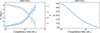 |
Fig. B.1. Left: The variation of the Tf (solid line) and γ (dashed line) as a function of the completeness limit in NGC4321. Error bars represent the fit scatter from running 100 random sampling bootstrap iterations on each completeness limit value. Right: Number of clouds (N) as a function of the completeness limit. |
Appendix C: The truncation limit
Our analysis follows that clouds follow a constant Tf per galaxy or environment for all clouds. However, as explained in Kobayashi et al. (2017), the mass-independent formulations overestimate the growth rate of very massive GMCs whose mass is comparable to the mass of a shell swept up by an expanding bubble. Thus, a truncation can be introduced in the form of Tf(m) = Tf[(1 + m/mtrunc)β] as explained in Section 4. Upon Taylor expansion, Tf(m) = Tf[(1 + βm/mtrunc)], and mcrit = mtrunc/β, where mcrit is the typical maximum GMC mass that can be created in the Inutsuka et al. (2015) evolution scenario. In Fig. C.1, we show how the age of a GMC varies when we add a truncation, where deviations start to occur at the more massive end of the mass spectrum (Mmol ≳ 106 M⊙), and thus we opt to fit without this truncation in our presented analysis. However, it is worth noting that the deviation is solely connected to the maximum GMC mass that can be swept up from a supernova remnant. Assuming multiple supernovae occur, or that the radius of the swept-up shell is greater than 100 pc, the truncation fit becomes closer to the GMC exponential growth fit that we used.
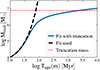 |
Fig. C.1. Left: Individual GMC Mmol as a function of Tage(m) following Eq. 6, where the black dashed line shows cloud exponential growth without a truncation, and the blue curve shows the cloud growth with a truncation mass of 7.7 × 10⁶ M⊙ (calculated for a shell of 100 pc radius and HI density of 10 cm−3; see expanding shell argument in Kobayashi et al. 2017). The truncation mass is shown with the dashed red line. |
Appendix D: The CO-to-H2 conversion factor
Comparison of truncated power-law fit parameters between SL24 (variable αCO; Schinnerer & Leroy 2024) and cst (constant αCO), where the percentage differences are computed as (SL24–cst)/cst.
In our analysis, we used the Schinnerer & Leroy (2024) prescription of the αCO conversion factor (see Sect. 3). However, multiple prescriptions exist and might bias the timescale estimates through the change of the slope γ of the GMC mass spectra. Therefore, to test if our analysis holds with another definition, we use a the constant Galactic  (K km s−1)−1, where R21 = 0.65 is based on Leroy et al. (2013) and den Brok et al. (2020), measured at kpc scales, and αCO(1 − 0) = 4.35 M⊙ pc−2 (K km s−1)−1 is the standard Galactic value at solar metallicity (i.e., Bolatto et al. 2013). Generally, as depicted in Table D.1, we find that γ and Tf only vary by less than 10 %, on average, upon adopting a different αCO prescription. Therefore, the results presented in the analysis are robust to the choice of αCO.
Appendix E: Additional Plots
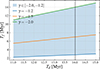 |
Fig. E.1. Tf as a function of Td for different γ indexes. The vertical dashed black line is the adopted value of Td = 14 Myr in our analysis. We vary γ from −1.2 to −2.0, which are the typical values across the galaxies, and note that Tf varies according to Tf = −(γ + 1)×Td. Thus, higher values of Td lead to more variation between Tf across the galaxies as depicted by the blue shaded regions. |
All Tables
Parameters of the truncated power-law fit of the GMC mass spectrum across the galaxies.
Spearman correlation coefficients (ρ) and p values between the GMC mass function slope γ and selected galactic/cloud properties across the 66 galaxies, ordered by decreasing |ρ|.
Median GMC formation timescales and ages by galactic environment across the galaxies.
Comparison of truncated power-law fit parameters between SL24 (variable αCO; Schinnerer & Leroy 2024) and cst (constant αCO), where the percentage differences are computed as (SL24–cst)/cst.
All Figures
|
Fig. 1. Example of the truncated power-law fit on NGC 0628. We present the fit on all clouds (global) and per galactic environment (center, S-arm, and I-arm). The vertical dashed line shows the completeness limit we set in our analysis. The dashed curve shows the truncated power-law fit. The fit parameters are presented in the box in the lower left region of each plot. |
| In the text | |
|
Fig. 2. Violin plots showing the distribution of the GMC mass spectra slope γ and Tf in increasing (Q1 to Q5) cloud-scale Σmol (left) and ΣSFR (right) bins within 66 (PHANGS Cycle 1 and 2) and 19 (PHANGS Cycle 1) galaxies, respectively. The upper x-axis shows the property median of each bin across the galaxies, with quantiles corresponding to the |
| In the text | |
|
Fig. 3. Scatter plots with error bars showing the variation in the median Tage(m) with log SFR (left) and log M★ (right) for the 66 galaxies in our sample. The black line shows the running median with the same number of galaxies in each bin, and the error is the standard error on the median. The Spearman correlation coefficient (ρ) is presented in each figure with the p value. Galaxies tend to have a longer cloud formation time with increasing SFR and M★. |
| In the text | |
|
Fig. 4. Bar plot with outliers (in circles) showing the exponential growth timescale, Tage(m), of GMCs across the galactic environment in 66 galaxies. The upper x-axis shows the median cloud Mmol with a 84th–50th and 50th–16th percentile distribution as upper and lower limits, respectively. The dashed black line represents the median timescale for all the clouds. On average, clouds with Mmol ≤ 105 M⊙ form in ≲20 Myr, with more massive clouds (106 − 7 M⊙) taking up to 100 Myr. Also, central clouds form the quickest compared to other environments by ∼0.3 dex. |
| In the text | |
|
Fig. 5. Growth time of the clouds, Tage(m), as a function of galactocentric radius for the sample of 66 galaxies split into grand-design spirals (prominent spiral features), non-grand-design spirals, and disk galaxies (no spiral features). The binned median per galaxy group is shown as solid lines, with error bars representing the standard error on the median (SE = |
| In the text | |
|
Fig. 6. Growth time of the clouds, Tage(m), as a function of galactocentric radius for the sample of 66 galaxies split according to galactic environment. The binned median per galaxy group is shown as solid lines, with error bars representing the standard error on the median. The solid black line represents the median trend for all the clouds regardless of galaxy group. All trends seem to be consistent with each other, with a ∼0.2 dex drop in the central regions. The scatterplot is a 2D histogram for the whole sample. |
| In the text | |
|
Fig. 7. Growth timescale as a function of Tdep (Eq. 15), Tff (Eq. 12), Torb (Eq. 13), and Tshear (Eq. 14). The median trend is plotted across galactic environments for the galaxies in our sample. The shaded region represents the 84th–50th, and 50th–16th percentiles, and the error bar is the standard error on the median. The Spearman correlation coefficient ρ is written in black when the correlation is significant (p < 0.05). Otherwise, it is not significant. |
| In the text | |
|
Fig. B.1. Left: The variation of the Tf (solid line) and γ (dashed line) as a function of the completeness limit in NGC4321. Error bars represent the fit scatter from running 100 random sampling bootstrap iterations on each completeness limit value. Right: Number of clouds (N) as a function of the completeness limit. |
| In the text | |
|
Fig. C.1. Left: Individual GMC Mmol as a function of Tage(m) following Eq. 6, where the black dashed line shows cloud exponential growth without a truncation, and the blue curve shows the cloud growth with a truncation mass of 7.7 × 10⁶ M⊙ (calculated for a shell of 100 pc radius and HI density of 10 cm−3; see expanding shell argument in Kobayashi et al. 2017). The truncation mass is shown with the dashed red line. |
| In the text | |
|
Fig. E.1. Tf as a function of Td for different γ indexes. The vertical dashed black line is the adopted value of Td = 14 Myr in our analysis. We vary γ from −1.2 to −2.0, which are the typical values across the galaxies, and note that Tf varies according to Tf = −(γ + 1)×Td. Thus, higher values of Td lead to more variation between Tf across the galaxies as depicted by the blue shaded regions. |
| In the text | |
Current usage metrics show cumulative count of Article Views (full-text article views including HTML views, PDF and ePub downloads, according to the available data) and Abstracts Views on Vision4Press platform.
Data correspond to usage on the plateform after 2015. The current usage metrics is available 48-96 hours after online publication and is updated daily on week days.
Initial download of the metrics may take a while.