


| Issue |
A&A
Volume 710, June 2026
|
|
|---|---|---|
| Article Number | A293 | |
| Number of page(s) | 19 | |
| Section | Planets, planetary systems, and small bodies | |
| DOI | https://doi.org/10.1051/0004-6361/202659296 | |
| Published online | 22 June 2026 | |
JWST high-contrast spectroscopy with speckle modelling: Atmospheric retrievals of the T-dwarf companion HD 19467 B
1
Leiden Observatory, Leiden University,
PO Box 9513,
2300 RA,
Leiden,
The Netherlands
2
Department of Astronomy & Astrophysics, University of California,
San Diego, La Jolla,
CA
92093,
USA
★ Corresponding author: This email address is being protected from spambots. You need JavaScript enabled to view it.
Received:
3
February
2026
Accepted:
30
April
2026
Abstract
Context. High-contrast medium-resolution spectroscopy with JWST can resolve molecular and isotopic features in cool substellar atmospheres, but for close-in companions, the extracted spectra can be biased by wavelength-dependent residual stellar contamination.
Aims. We assess the impact of residual speckles on atmospheric inference for the T-dwarf companion HD 19467 B and compare the results to those for the field T dwarf 2MASS J0415−0935.
Methods. We analysed JWST/NIRSpec G395H spectra (2.87–5.2 µm; R ∼ 2700) and performed Bayesian atmospheric retrievals with petitRADTRANS coupled with nested sampling using ultranest. We used a flexible parametrised pressure–temperature profile with free constant-with-altitude molecular abundances. For HD 19467 B, we fitted the PSF-subtracted spectrum with a linear model that included the atmospheric model and a set of speckle spectra from the integral field unit.
Results. We detected H2O, CH4, CO, CO2, and NH3 in both atmospheres and measured carbon isotopic ratios from CO isotopologues, finding 12C/13C = 154−17+19 for HD 19467 B and 12C/13C = 85 ± 5 for 2MASS J0415−0935. Speckle contamination primarily affects the low-frequency spectral shape at 3.0–3.7 µm and can affect the retrieved abundances when it is not accounted for. We obtained apparently constrained posteriors for some additional species (e.g. SiO and H2S) in some cases, but treated them as tentative because a cross-correlation yielded no significant detections; PH3 is not detected in either target.
Conclusions. A joint fitting of the atmospheric spectrum and the speckle contamination enabled us to perform native-resolution retrievals of the high-contrast companion HD 19467 B with JWST/NIRSpec without continuum subtraction. Over 2.87–5.2 µm medium-resolution spectroscopy constrains the elemental and isotopic composition. Both objects exhibit near-solar metallicity and subsolar C/O ratios.
Key words: instrumentation: spectrographs / planets and satellites: atmospheres / brown dwarfs
© The Authors 2026
 Open Access article, published by EDP Sciences, under the terms of the Creative Commons Attribution License (https://creativecommons.org/licenses/by/4.0), which permits unrestricted use, distribution, and reproduction in any medium, provided the original work is properly cited.
This article is published in open access under the Subscribe to Open model. This email address is being protected from spambots. You need JavaScript enabled to view it. to support open access publication.
1 Introduction
Brown dwarfs have masses below the hydrogen-burning limit and bridge the gap between giant planets and low-mass stars. As brown dwarfs evolve and cool, their atmospheres become rich in molecules and condensates. This shapes their spectra in the M, L, T, and Y classes (Kirkpatrick et al. 1999; Burrows et al. 2001; Cushing et al. 2005). The overlap in effective temperatures between brown dwarfs and directly imaged exoplanets makes them a valuable laboratory for the physics and chemistry that govern planetary atmospheres Faherty et al. (2016).
During the brown dwarf cooling sequence, the L/T transition marks a major change in atmospheric appearance that is commonly linked to cloud structure and dynamics (Burgasser et al. 2002b; Gao et al. 2018). Older objects with a higher gravity often exhibit largely cloud-free photospheres, with clouds thought to sink to deeper atmospheric layers (Allard et al. 2001; Saumon & Marley 2008). Conversely, younger objects with a lower gravity often exhibit cloudier atmospheres, with condensates present at or above the photosphere (Ackerman & Marley 2001; Burrows et al. 2006). A further hallmark is the increase in CH4 at the expense of CO as temperatures fall below ∼1500 K (e.g. Zahnle & Marley 2014). Disequilibrium chemistry can inhibit CO→CH4 conversion, leaving detectable CO in cool T dwarfs and providing a diagnostic of atmospheric mixing timescales (e.g. Fegley & Lodders 1996; Moses et al. 2011).
T dwarfs show prominent H2O, CH4, and NH3 absorption in the infrared, with frequent evidence of CO (e.g. Burgasser et al. 2002a; Burrows et al. 2003; Calamari et al. 2022). The presence of CO in the spectra of T dwarfs indicates disequilibrium chemistry, as was first identified in Jupiter (Prinn & Barshay 1977; Bézard et al. 2002). Historically, most spectroscopy of brown dwarfs was obtained from the ground between 1 and 2.5 µm. The 3–5 µm window, which carries critical information on CH4, H2O, NH3, CO, and CO2, is challenging from the ground because the thermal background is high, but was accessed by space-based facilities such as Spitzer (Cushing et al. 2005) and the infrared satellite AKARI (Sorahana et al. 2013). The advent of JWST has transformed the field of brown dwarf atmospheres. Medium-resolution spectroscopy beyond 3 µm at unprecedented sensitivity and stability (Rigby et al. 2023) is now possible for objects that are too faint for ground-based facilities. Recent observations of brown dwarfs with NIRSpec and MIRI demonstrate the remarkable data quality achievable at these wavelengths (Miles et al. 2023; Hood et al. 2024; Hoch et al. 2024).
Despite JWST’s stability and sensitivity, it remains challenging to characterise close-in companions because of the high contrast and structured point-spread functions. Robust modelling and subtraction of the host-star point-spread function (PSF) are essential to unlock medium-resolution spectroscopy with the NIRSpec IFU at small angular separations. Building on moderate-resolution high-contrast methods developed from the ground, Ruffio et al. (2024) demonstrated advanced PSF modelling and companion extraction that improved the sensitivity at small to moderate separations (i.e. 300–2000 mas). These strategies are directly relevant to systems such as HD 19467, where high-contrast techniques are essential to obtain spectroscopy of companions at small angular separations (Maire et al. 2020; Ruffio et al. 2024). The imperfect subtraction of diffracted starlight can leave a significant imprint on direct-imaging datasets. This is often referred to as speckles (Currie et al. 2023). A central goal of current high-contrast instrumentation and post-processing is therefore to mitigate and quantify speckle residuals to enable a reliable characterisation of faint companions at progressively smaller separations (Ruffio & Pueyo 2026).
The wealth of spectral features in brown dwarf atmospheres enables us to characterise atmospheric composition, structure, and dynamics in detail. The analysis of chemical abundances is key to understanding the formation pathways of brown dwarfs and planets. The elemental ratios and bulk metallicity encode the relative contributions of gas and solids accreted during formation and may be linked to the birth location (Öberg et al. 2011; Madhusudhan 2019; Mollière et al. 2022; Zhang 2020; Fortney 2012). Recent work on carbon, oxygen, and sulfur ratios in a multi-planet system revealed super-stellar ratios similar to those of Jupiter, suggesting that the enrichment pathways of Solar System gas giants might be applicable to super-Jupiters such as the HR 8799 planets (Ruffio et al. 2026). Isotope ratios have been proposed as complementary tracers of formation pathways (Mollière & Snellen 2019; Zhang et al. 2021a). Isotopologues of carbon monoxide such as 13CO and C18O have been measured for a number of brown dwarfs and directly imaged planets (Zhang et al. 2021b; Gandhi et al. 2023; Xuan et al. 2024; Grasser et al. 2025). These measurements provide valuable insights into the birth environment and potential accretion of solids into the atmosphere, and they can be used to separate the formation pathways of planets and brown dwarfs (Zhang et al. 2021a). The distinct carbon isotope ratios in the HR 8799 planets (Ruffio et al. 2026) suggest that isotopic abundances might vary as a function of birth location within the same system.
The large number of molecular features in the spectra of sub-stellar objects requires a detailed modelling of the temperature and chemistry of the atmosphere. Traditionally, grids of forward models incorporating radiative-convective thermochemical equilibrium, condensation, and non-equilibrium chemistry are used to predict spectra for a small set of fundamental parameters (Allard et al. 2012; Marley et al. 2021). However, these models are limited by the number of free parameters and the assumptions made about the chemistry and physics of the atmosphere. A complementary approach is to use data-driven retrievals to infer molecular abundances and bulk properties directly from the observations, as originally developed for planetary sciences (Rodgers 2000; Irwin et al. 2008).
The forward models used in atmospheric retrievals typically incorporate minimal physical constraints, and are able to adjust the temperature structure and composition of the atmosphere to fit the observations (e.g. Line et al. 2015; Burningham et al. 2017; Mollière et al. 2020). Retrievals are typically performed using a Bayesian framework, and the resulting posterior distributions of the free parameters are used to interpret the properties of the atmosphere. The number of free parameters in the retrieval is typically much larger than the number of free parameters in the forward model (e.g. de Regt et al. 2024). Despite this, atmospheric retrievals have been very successful at fitting the near-infrared spectra of brown dwarfs to high precision, even in situations where additional physical processes were needed to explain the observations (e.g. thermal inversions; Faherty et al. 2024).
2 Data
We analysed spectra of two well-studied T dwarfs: the high-contrast companion HD 19467 B, and the nearest known isolated T dwarf 2MASS J0415−0935. The comparative analysis of the two objects probes the effect of residual speckles in the 2.9–5.3 µm spectrum of HD 19467 B and highlights the modelling limitations for T-dwarf atmospheres.
2.1 HD 19467 B
HD 19467 B is a brown dwarf companion to the G3V star HD 19467, discovered through the TRENDS high-contrast imaging survey (Crepp et al. 2014). This system has been extensively characterised through multiple observational campaigns, providing one of the most comprehensive datasets for a substellar companion.
The companion was first detected through Keck/NIRC2 coronagraphic imaging combined with long-baseline radial velocity measurements, establishing a firm dynamical lower limit on the companion mass (Crepp et al. 2014). Low-resolution ground-based spectroscopy confirmed the T-dwarf nature with a spectral classification of T5.5 ± 1 (Crepp et al. 2015).
Subsequent high-contrast imaging with VLT/SPHERE and NaCo, combined with archival data and joint orbital fitting, refined the dynamical mass estimates (Maire et al. 2020). The most recent analysis incorporating JWST astrometry and orbital constraints yields an updated dynamical mass of  MJ (Hoch et al. 2024). The orbital characterisation by Maire et al. (2020) showed that HD 19467 B is in a long-period high-eccentricity orbit.
The host star age is old (8–10 Gyr; Maire et al. 2020; Greenbaum et al. 2023), making HD 19467 B a rare target for high-contrast spectroscopy of an old, cool brown dwarf.
Observations by the IFU on JWST/NIRSpec of HD 19467 B were obtained as part of Cycle 1 GTO programme 1414 (PI: Marshall Perrin) targeting high-contrast companions. We used the companion spectrum as extracted and processed by Ruffio et al. (2024). Using a reference-star PSF subtraction (reference differential imaging; RDI), they extracted the first moderate-resolution spectrum of HD 19467 B between 2.9–5.3 µm at a signal-to-noise ratio (S/N) of ∼10 in the continuum. The reduction used the JWST calibration pipeline (v1.10.2) to generate flux-calibrated detector images, with stellar PSF subtraction and flux extraction performed directly on the detector images rather than reconstructed spectral cubes (Ruffio et al. 2024); the same extracted spectrum was analysed with atmospheric grids by Hoch et al. (2024). The extracted spectra of both targets are shown in Fig. 1.
2.2 2MASS J0415-0935
The T8 dwarf 2MASS J04151954−0935066 (2M 0415 hereafter) was discovered by Burgasser et al. (2002a). It has become a standard for the spectral classification of late-type cool T dwarfs. This object has been extensively studied in multiple wavelength regimes, making it a useful reference object for atmospheric modelling (e.g. Leggett et al. 2007; Yamamura et al. 2010; Hood et al. 2024; Alejandro Merchan et al. 2025).
Discovered in the 2MASS survey, 2M 0415 is a nearby (5.71 ± 0.06 pc; Dupuy & Liu 2012) late-T dwarf (T8). Its near-infrared magnitudes are J = 15.34 and H = 15.67, and its near-infrared spectrum shows the strong CH4 and H2O absorption characteristic of late-T dwarfs (Burgasser et al. 2002a).
Mid-infrared spectroscopy with Spitzer/IRS (5–20 µm) and Subaru/IRCS (2.9–4.1 µm) provided key constraints on the spectral energy distribution (Cushing et al. 2005; Saumon & Marley 2008). Model fits to these data yielded the first comprehensive estimates of the fundamental parameters that were later broadly confirmed by subsequent studies (Saumon & Marley 2008; Filippazzo et al. 2015). More recently, near-complete SED analyses of 2M 0415 have delivered some of the most precise fundamental-parameter constraints for any T dwarf by combining the same G395H dataset analysed here with additional data spanning ∼1–20 µm (Hood et al. 2024; Alejandro Merchan et al. 2025).
Observations with JWST/NIRSpec of 2MASS J0415−0935 were obtained in Cycle 1 GO programme 2124 (PI J. Faherty) using the G395H grating and F290LP filter, covering 2.87–5.14 µm at R ≈ 2700. The data and a detailed analysis were presented by Hood et al. (2024), who performed grid-based fits and combined the NIRSpec spectrum with lower-resolution spectra (i.e. IRTF/SpeX and Spitzer/IRS) in a full SED retrieval. The resulting parameters agree well with earlier determinations and have substantially reduced the uncertainties (see Section 5).
The NIRSpec spectrum shows prominent bands of H2O, CH4, CO2, and CO. In particular, strong CO absorption at 4.6–5.0 µm indicates disequilibrium chemistry, consistent with earlier lower-resolution evidence from AKARI (Yamamura et al. 2010). The spectrum also covers the ν1 band of NH3 near 3 µm, which was previously identified in JWST low-resolution data of the Y0 dwarf WISE J035934.06−540154.6 (Beiler et al. 2023).
 |
Fig. 1 Spectrum obtained with JWST NIRSpec of HD 19467 B and 2MASS J0415−0935. The flux has been scaled for plotting purposes to a reference spectrum of a 1 RJup object at 10 pc. The data for detectors NRS1 (panel a) and NRS2 (panel b) are shown. The different wavelength coverage is due to the different observing setups for the two objects (i.e. IFU and fixed slit). Molecular opacity is overlaid for a reference temperature and pressure of 900 K and 2 bar. The opacity was calculated using the retrieved volume mixing ratios for the detected species, and for non-detections, we used reference values from the models (i.e. PH3). |
3 Methods
3.1 Atmospheric modelling
We computed high-resolution emission spectra with petitRADTRANS v3.1 (Mollière et al. 2019; Blain et al. 2024). The line opacities were taken from petitRADTRANS where available or were generated with pyROX1 (de Regt et al. 2025) using the latest line lists (Gordon et al. 2022; Tennyson et al. 2024). We used the following line lists for 12CH4 (Yurchenko et al. 2024), 13CH4 (Gordon et al. 2022), CH3D (Rothman et al. 2013),  (Polyansky et al. 2018),
  (Polyansky et al. 2017), CO isotopologues (Rothman et al. 2010; Li et al. 2015), NH3 (Coles et al. 2019), 12CO2 and 13CO2 (Hargreaves et al. 2025), SiO (Yurchenko et al. 2022), H2S (Azzam et al. 2016; Chubb et al. 2018), and PH3 (Sousa-Silva et al. 2015).
The model spectra were generated at a resolving power of R=100 000 and were subsequently convolved to the instrumental resolution of NIRSpec using a wavelength-dependent Gaussian kernel whose full width at half maximum (FWHM) is set by the NIRSpec calibration files (see also González Picos et al. 2025a2). Recent in-flight measurements suggest that the actual resolving power may be higher by 1–24% (Shajib et al. 2025). The resolving power could alternatively be parametrised and fitted (Gandhi et al. 2023; Ruffio et al. 2026); we nevertheless fixed it to the calibration values for simplicity. This choice reproduces the observed line shapes well, as evidenced by the quality of the fit and the shape of the cross-correlation functions (see Figs. 3 and B.1).
We adopted a flexible atmospheric retrieval framework in which we retrieved a parametrised pressure–temperature profile together with constant-with-altitude molecular abundances. The model spectra were generated with petitRADTRANS using the same line lists and resolving power throughout.
The free parameters were the radius, mass or log g, the radial velocity (one per detector; Appendix F), an error-inflation parameter, molecular abundances, and the isotopologue ratios. For HD 19467 B, we used the dynamical mass  MJup (Hoch et al. 2024) as a Gaussian prior (truncated at 2σ with scipy.stats.truncnorm3); this was our default configuration throughout the paper. The surface gravity was then derived from the retrieved radius and mass. The dynamical constraint breaks the well-known degeneracy between log g and metallicity in medium-resolution retrievals of cool T dwarfs (see Section 5.2 for a discussion of the unconstrained case). For 2M 0415, which lacks a dynamical mass, we retrieved log g directly as a free parameter. The complete list of retrieved parameters and priors is given in Table C.1.
The pressure–temperature profile was parametrised with free temperature gradients and pressure levels following González Picos et al. (2025a) based on Zhang et al. (2023). The temperature at each atmospheric layer Tj was calculated from the temperature gradients, which were linearly interpolated from the gradients at the reference points ∇i and the pressure levels Pi with i = 0, 1,…, 6,
 (1)
(1)
where T0 is the surface temperature at 100 bar. The pressure levels were fixed at the bottom (P0 = 100 bar) and top (P6 = 10−4 bar) of the atmosphere; the intermediate levels were set by the free parameters log PRCE and ∆ log P via log Pi = log PRCE + x(i) · ∆ log P with x(i) = −2, −1, 0, 1, 2 for i = 1,…, 5. The composition was modelled with constant-with-altitude volume mixing ratios, with a free parameter for each molecule (except for minor isotopologues, which were fitted via ratios with the main isotopologues).
From the individual abundances, we calculated the gas-phase C/O ratio as
 (2)
(2)
The gas-phase abundances neglect any elemental reservoirs in condensates (e.g. oxygen sequestration into silicates; Burrows & Sharp 1999; Line et al. 2017). As a result, (C/O)gas can overestimate the bulk C/O ratio when condensation is high. To facilitate comparisons to bulk compositions, we estimated the bulk C/O and O/H using empirical corrections (Calamari et al. 2024; Kothari et al. 2026). Specifically, we adopted an oxygen condensation fraction fO = 0.371 (Calamari et al. 2024), such that
 (3)
(3)
![Mathematical equation: ${\left( {{\rm{O/H}}} \right)_{{\rm{bulk}}}} = {\left( {{\rm{O/H}}} \right)_{{\rm{gas}}}}\left[ {1 - {f_{\rm{O}}}{{\left( {{\rm{C/O}}} \right)}_{{\rm{bulk}}}}} \right].$](/articles/aa/full_html/2026/06/aa59296-26/aa59296-26-eq9.png) (4)
(4)
We note that a typo in Equation (11) of Kothari et al. (2026) is corrected here. When not explicitly stated, the abundances should represent the bulk composition throughout the present work. We report elemental ratios with respect to the solar values as
![Mathematical equation: $\left[ {{\rm{X/H}}} \right] = {\log _{10}}\left( {{\rm{X/H}}} \right) - {\log _{10}}{\left( {{\rm{X/H}}} \right)_ \odot },$](/articles/aa/full_html/2026/06/aa59296-26/aa59296-26-eq10.png) (5)
(5)
with abundances from Asplund et al. (2021). To derive effective temperatures from the posteriors, we computed a low-resolution spectrum (λ/∆λ = 100) for each posterior sample over 0.3– 28 µm and integrated it to obtain the bolometric flux,
 (6)
(6)
with λ1 = 0.3 µm and λ2 = 28 µm. Outside the G395H window, we included additional opacity sources relevant at shorter wavelengths (TiO, VO, FeH, HCN, Na, and K), adopting chemical equilibrium abundances at the corresponding bulk C/O and metallicity (using [C/H] as a proxy). We then computed Teff = (Fbol/σSB)1/4. Additional opacity sources not included here (in particular, oxides and hydrides at bluer optical and near-infrared wavelengths; e.g. MgO, CrH) might bias Fbol if they are significant absorbers and thus shift Teff to lower values. We therefore report Teff primarily as a consistency check, but we note that the most robust constraints on fundamental parameters come from full SED observations and analyses.
3.2 Speckle modelling for HD 19467 B
Because the PSF subtraction is imperfect, residual starlight (also referred to as speckles) is present in the companion spectrum. This residual signal exhibits a small non-zero mean that was subtracted from the companion spectrum as described in Ruffio et al. (2024). Residual contamination from the host star was therefore not fully removed at the companion position and might bias the retrieval of atmospheric parameters if it is not accounted for. In some cases, stray light leaked into the instrument and produced bright stripes across the detector. These stripes also referred to as ghosts (see panel b of Fig. 2 and Ruffio et al. (2024) for more details).
For HD 19467 B, we implemented a speckle-modelling approach using a linear model framework that included the atmospheric signal and a set of speckle model spectra. The speckle spectra used here were provided by Ruffio et al. (2024)4 and were extracted from an annular region (0.3–0.4 arcseconds) around the companion. This is an alternative to using a covariance matrix to model the speckle structure (Greco & Brandt 20160), which is implemented in Ruffio et al. (2024).
We calculated the dominant modes of the speckle spectra using a principal component analysis (PCA) decomposition (see Fig. 2, also Hoeijmakers et al. 2018). The speckle model was defined by smoothing the PCA components with a Gaussian filter (51 pixels) and retaining N = 30 components. We tested a range of filter widths and component numbers by iteratively performing linear fits on the best-fit model from an initial retrieval. We found that the selected number of components and filter width captured 90% of the variance in the speckle spectra and that the results were not very sensitive to further optimisation. We used the same number of components for all detectors, but we note that the linear fit was performed on each detector separately. We refrained from further optimisation of the speckle model (i.e. filter width and number of components for each detector) to avoid overfitting and to preserve the simplicity of the model. The speckle field we used to construct the speckle basis is shown in Fig. 2.
 |
Fig. 2 Speckle spectral field for HD 19467 B. a. The annular slice of the integral field unit used to extract the speckle model spectra was adopted from Ruffio et al. (2024). b. Spectra from individual pixels in the annular slice of the IFU (n = 120 pixels). c. PCA reconstruction of the speckle spectra with 30 components. From top to bottom, we show the components with the largest fitted amplitudes. d. Amplitude of the five speckle components with the largest amplitude from the joint atmospheric and speckle fit. e. Combined speckle model from the best-fit retrieval. |
3.3 Bayesian retrieval framework
We employed a Bayesian retrieval framework to determine atmospheric parameters from the observed spectra. For 2M 0415, the residuals between the atmospheric model and the data were computed directly and the likelihood was evaluated with Equation (12). For HD 19467 B, a few additional steps were required to account for residual speckle contamination. We used a linear model that included the planetary signal and a set of speckle model spectra, following the approach of Wilcomb et al. (2020); Landman et al. (2024).
The model is expressed as
 (7)
(7)
where d is the spectrum extracted at the companion position, M is the model matrix, ϕ is the vector of linear coefficients, and n is Gaussian-distributed noise with zero mean and covariance matrix Σ. The coefficient ϕ0 scales the companion model, and ϕ1…N scale the speckle components. The column M0 is the atmospheric model of the companion generated with petitRADTRANS, and M1…N are the speckle components derived from PCA decomposition of the annular region spectra.
The covariance incorporates an error-inflation parameter b that accounts for systematic uncertainties beyond the formal errors. The effective variance for each data point is
 (8)
(8)
where σi is the formal uncertainty for the ith data point. We adopted a diagonal covariance,  , which in preliminary tests captured the residual structure without additional correlated-noise parameters.
When speckle correction was applied, we solved for the optimal speckle coefficients ϕspeckles using a least-squares solver5,
 (9)
(9)
where r = f − s denotes the residuals between the observed flux f and the model spectrum s. The corrected residuals are then
 (10)
(10)
Because the amplitude of the atmospheric model is set by the radius, the speckle amplitudes were fitted after subtracting the atmospheric model.
The χ2-statistic is computed as
 (11)
(11)
where r denotes either the original or speckle-corrected residuals r′, and N is the number of valid data points. The log-likelihood is given by
 (12)
(12)
where |Σ| is the determinant of the covariance matrix. The optimal linear parameters  and noise scaling factor
  are obtained by minimising χ2.
We used nested sampling for the posterior exploration and evidence computation (ultranest; Skilling 2004; Buchner 2021). We adopted 1000 live points and a convergence criterion of ∆ ln Z = 0.5, using a mixed-mode step sampler (Buchner 2023, 2022). For HD 19467 B, we verified consistency with PyMultiNest in constant-efficiency mode (Fig. G.1).
3.4 Detection of minor species
We assessed the detectability of minor species (e.g. SiO and C18O) by removing each species from the best-fit free model and quantifying the preference for inclusion using the Akaike information criterion (AIC; Akaike 1974). We defined ∆AIC ≡ AIC(no molecule) − AIC(baseline), where positive values favour inclusion. The detection significance was estimated using the criterion of Thorngren et al. (2026). While an evidence-based comparison would be more robust, full Bayesian retrievals for each species are unfeasible given the computational cost (∼104 CPU hours per retrieval).
 |
Fig. 3 Best-fit model spectrum for HD 19467 B. We show the individual contributions from the atmospheric model and the speckle model. The selected opacity sources are indicated in the relevant wavelength regions. The equivalent figure for 2M 0415 is shown in Fig. A.1. The data products required to reproduce this figure are available on Zenodo (González Picos et al. 2026). |
4 Results
We present atmospheric retrieval results for HD 19467 B and 2M 0415 using the framework described in Section 3.1. For HD 19467 B, we adopted the dynamical mass of Hoch et al. (2024) as a Gaussian prior; this was our default configuration and the one we discuss throughout. The effect of dropping the mass prior is discussed in Section 5.2. For 2M 0415, no dynamical mass is available, and log g was a free parameter. We focus on the spectral fits, atmospheric structure, molecular abundances, and isotopic ratios inferred from the G395H data.
Fig. 3 shows the best-fit spectrum of HD 19467 B and highlights the contribution of residual speckle contamination. Fig. A.1 shows the best-fit spectrum for 2M 0415. In Fig. 4 we compare our best-fit model spectrum for HD 19467 B with Hoch et al. (2024). Fig. 5 summarises the best-fit temperature profiles, emission contribution functions, and retrieved compositions for both targets. The posterior probability distributions are shown in Fig. D.1 for HD 19467 B and in Fig. E.1 for 2M 0415. The isotopologue posteriors are shown in Fig. 6, and a full list of the retrieved parameters is provided in Table C.1.
 |
Fig. 4 Comparison of our best-fit model spectrum for HD 19467 B in two selected wavelength regions with the best-fit model from Hoch et al. (2024) using a custom NewEra model grid (Hauschildt et al. 2025). |
4.1 Spectral fits
We fitted the full JWST/NIRSpec G395H spectra of HD 19467 B and 2M 0415 and achieved a residual scatter comparable to the S/N of the data with error-scaling factors of s = 1.10 and s = 1.99, respectively (typical uncertainty ±0.02). The joint spectrum and speckle linear model reproduces the native-resolution data for HD 19467 B without requiring continuum subtraction (see Fig. 3 and Section 5.1).
4.2 Temperature–pressure profile
The temperature-pressure profiles of the two objects are well constrained by the data, as shown in Figure 5.
Our pressure-range sensitivity, as represented by the emission contribution function in Fig. 5, extends from approximately 10 to 0.01 bar.
4.3 Chemical composition
We report detections of H2O, CO, CH4, NH3, and CO2 in the atmospheres of HD 19467 B and 2M 0415. We found constrained posterior distributions for the abundances of all these species (see Figs. D.1 and E.1) and significant cross-correlation peaks (S/N > 3; see Fig. B.1).
Additionally, our retrievals appear to constrain the abundance of SiO in HD 19467 B, but find only weak evidence for its presence in 2M 0415. This is discussed in more detail in Section 5.4. In both cases, however, the cross-correlation analysis yields no significant detection of SiO (S/N < 3; Fig. B.1), and we therefore treat any apparent constraints on SiO as tentative. We also constrained the abundances of minor isotopologues including 13CO C18O and tentative evidence for H218O. We assess the potential presence of 13CH4 and 13CO2 in Section 5.3.
Figure 5 (right column) shows the volume-mixing ratios of the detected species as a function of pressure compared with Sonora elf owl models (Mukherjee et al. 2024; Wogan et al. 2025). Both objects exhibit moderate vertical mixing, with log Kzz ≈ 3–4 dex, required to reconcile the observed CO absorption features and volume-mixing ratios. The balance of the chemical timescales at lower pressures drives the atmosphere out of chemical equilibrium, thereby inhibiting the conversion of CO into CH4 and preserving a relatively high abundance of CO compared to chemical equilibrium predictions (Zahnle & Marley 2014). CO2 is also significantly sensitive to Kzz: vertical mixing can transport CO2 from deeper, hotter layers into the photosphere, potentially enhancing its observable abundance (Wogan et al. 2025; Beiler et al. 2024). We detect CO2 in both objects, with abundances consistent with the updated Sonora elf owl model atmospheres (Beiler et al. 2024000; Wogan et al. 2025).
We report elemental ratios including the empirical correction for oxygen sequestration (see Section 3.1),
![Mathematical equation: $\matrix{ {{{\left[ {{\rm{C/H}}} \right]}_{{\rm{HD 19467 B}}}}} \hfill & = \hfill & {0.14_{ - 0.04}^{ + 0.04},} \hfill & {{{\left[ {{\rm{C/H}}} \right]}_{{\rm{2M 0415}}}}} \hfill & = \hfill & {0.15_{ - 0.07}^{ + 0.09}} \hfill \cr {{{\left[ {{\rm{O/H}}} \right]}_{{\rm{HD 19467 B}}}}} \hfill & = \hfill & {0.18_{ - 0.04}^{ + 0.05},} \hfill & {{{\left[ {{\rm{O/H}}} \right]}_{{\rm{2M 0415}}}}} \hfill & = \hfill & {0.11_{ - 0.08}^{ + 0.09}} \hfill \cr {{\rm{C/}}{{\rm{O}}_{{\rm{HD 19467 B}}}}} \hfill & = \hfill & {0.389_{ - 0.012}^{ + 0.012},} \hfill & {{\rm{C/}}{{\rm{O}}_{{\rm{2M 0415}}}}} \hfill & = \hfill & {0.451_{ - 0.006}^{ + 0.005} \cdot } \hfill \cr } $](/articles/aa/full_html/2026/06/aa59296-26/aa59296-26-eq21.png) (13)
(13)
The carbon and oxygen abundances are slightly super-solar for both objects, while the C/O ratios are sub-solar (C/O⊙ = 0.59 ± 0.08; Asplund et al. 2021). Our C/O value for HD 19467 B is consistent with previous ground-based measurements from Mesa et al. (2020) (C/O=0.36 ± 0.03). For 2M 0415, our C/O value is lower than the full SED retrieval from Hood et al. (2024) (C/O=0.53 ± 0.01; corrected for oxygen condensation similar to our empirical correction), but we note that in the same study, the authors also found lower C/O values when using Sonora elf owl models (C/O=0.36 ± 0.002).
5 Discussion
5.1 Speckle contamination in HD 19467 B
The high-contrast nature of the HD 19467 B system necessitates a careful treatment of residual stellar contamination in the extracted companion spectrum. At a separation of 1.6 arc-seconds, the flux ratio of the companion and host star ranges from 10−5 to 10−6 across 3–5 µm. Despite the PSF-subtraction approach described in Ruffio et al. (2024), speckle contamination remains a significant systematic that must be addressed to correctly fit the spectrum and interpret atmospheric parameters. We identified this contamination after numerous attempts to extend our atmospheric model to include additional effects that might account for the clear mismatch between data and model around 3.0–3.7 µm. This discrepancy was independently noted by Hoch et al. (2024), who fitted the same dataset with four different self-consistent models and found a similar mismatch in all cases (see Fig. 4). To mitigate this issue, Hoch et al. (2024) removed the continuum from the data and model, but this approach resulted in information loss and may not eliminate the speckle contamination on the spectral features.
Speckle contamination predominantly affects the low-frequency spectral continuum, with the most severe residuals concentrated in the 3.0–3.7 µm interval (see Fig. 3). Speckle residuals are smaller at 4.3–5.2 µm but remain non-negligible and can still bias the inferred abundances. Omitting the speckle component from our retrieval yields a dramatically worse fit (disfavoured at ∼60σ; Fig. 4) and introduces systematic biases in the retrieved parameters, including a smaller inferred radius, the non-detection of NH3, a spurious H2S detection, and inaccurate isotopic abundance ratios (Fig. D.1). Simply excluding the 3.0–3.7 µm region reduces the apparent residuals, but does not prevent these biases, as speckle contamination persists throughout the full wavelength range.
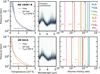 |
Fig. 5 Atmospheric structure of HD 19467 B and 2M 0415 from the free retrievals. Left: temperature profiles. The pressure and temperature range of the photosphere (emission contribution function >1%) is indicated by the error bars. Middle: emission contribution function. The dark regions indicate a high contribution. Right: Volume-mixing ratios. The arrows indicate the upper limits for the abundances of non-detected species. Sonora elf owl models (Mukherjee et al. 2024; Wogan et al. 2025) are overlaid for the temperature and volume-mixing ratios assuming a common metallicity of [M/H] = 0.2, a default C/O=0.458, and moderate vertical mixing, log Kzz = 3, which yields photospheric abundances broadly consistent with the retrievals. For HD 19467 B, we used Teff = 1000 K and log g = 5.5, and for 2M 0415, we used Teff = 700 K and log g = 5.0. |
5.2 Fundamental parameters
We computed Teff from the bolometric flux inferred by integrating low-resolution model spectra over 0.3–28 µm (see Section 3.1). The retrieved radii and masses are summarised in Table C.1. The quoted radii primarily capture the statistical uncertainties from the retrieval. An additional systematic uncertainty arises from the absolute flux calibration of NIRSpec, which is typically at the 5–10% level for spectroscopy6.
For HD 19467 B, our default retrieval used the dynamical mass of Hoch et al. (2024) as a Gaussian prior, yielding a surface gravity log g = 5.45 ± 0.03 consistent with an old, high-gravity brown dwarf and near-solar metallicity (Table 1).
Comparison to previous analyses of HD 19467 B (Table 1), Greenbaum et al. (2023) found a significantly smaller radius (and correspondingly lower luminosity) than expected for an old brown dwarf, while Hoch et al. (2024) derived a dynamical mass consistent with earlier orbit-based estimates and argued for stronger vertical mixing. Medium-resolution long-slit spectroscopy of HD 19467 B with SPHERE/IRDIS by Mesa et al. (2020) yielded an independent spectral characterisation (T6±1) and atmospheric parameters that are broadly consistent with a cool (Teff ∼ 1000 K), high-gravity (log g ∼ 5) object. Our inferred Teff ∼ 1080 K agrees well with the effective-temperature scale found in these studies.
For completeness, we also performed a retrieval without the mass prior: this led to a lower surface gravity and a mass significantly lower than the dynamical constraint (around 20 MJup) with a slightly (∼4σ) improved fit, but this is likely a way for the model to compensate for other mismatches between data and model. All parameters are consistent within 1σ except for the surface gravity and the abundances, which are shifted accordingly due to the metallicity–surface gravity degeneracy. This results in a very low metallicity (∼−0.50), an effect also observed in this type of analysis of other objects. Inclusion of the mass prior therefore adds relevant information to correctly interpret the abundances and fundamental parameters, and we adopted the mass-constrained retrieval as our default throughout.
For 2M 0415, the inferred fundamental parameters and literature comparisons are summarised in Table 1. Despite the limited wavelength coverage, our G395H-only inference yields an Lbol and Teff consistent with full SED analyses (Hood et al. 2024; Alejandro Merchan et al. 2025). In particular, the near-complete SED analysis of Alejandro Merchan et al. (2025) should provide the most direct constraints on fundamental parameters owing to its extended wavelength coverage, which are consistent with our inferred parameters within 1σ. This agreement suggests that the 2.87–5.27 µm window already captures much of the information needed to constrain the bolometric flux and effective temperature of this object. However, the smaller uncertainties of our analysis do not account for the assumptions made outside the wavelength range of the G395H window, which may introduce additional systematic uncertainties. We recommend the use of full SED analyses for more precise constraints on fundamental parameters.
 |
Fig. 6 Posterior distributions of the isotopologue ratios for HD 19467 B (top; with dynamical mass prior) and 2M 0415 (bottom). The values of the ISM (68 ± 15; Milam et al. 2005) and solar (93.5 ± 3.1; Lyons et al. 2018) are shown for reference. |
Summary of the fundamental parameters.
5.3 Isotopic ratios
We inferred the carbon and oxygen isotope ratios from CO and H2O isotopologues (Figure 6). We quote the CO-based ratios (higher sensitivity) and find consistent constraints from H2O. We find
 (14)
(14)
The ratios of the two objects are higher than solar (12C/13C⊙ = 93±3, 16O/18O⊙ = 525±21; Ayres et al. 2013; Lyons et al. 2018), and the ratio of HD 19467 B is higher than that of 2M 0415. This is qualitatively consistent with the galactic chemical evolution: older systems are expected to show higher 12C/13C and 16O/18O as the ISM becomes enriched in 13C and 18O (Prantzos et al. 1996; Romano 2022). Given the broad age estimates for 2M 0415 (1–8 Gyr; Hsu et al. 2021; Hood et al. 2024; Alejandro Merchan et al. 2025), our measurements suggest that it is younger than the 8–10 Gyr HD 19467 system and might be closer to the age of the Sun (Bouvier & Wadhwa 2010). Similarly high ratios have been reported for old M dwarfs (Crossfield et al. 2019; González Picos et al. 2025b).
We also tested 13CH4, 13CO2 and CH3D. 13CH4 is only tentatively detected; for HD 19467 B, the strongest feature (3.32 µm) overlaps strong speckle residuals (Figure 7), likely biasing the inferred 12C/13C. 13CO2 is not detected in HD 19467 B and is weakly constrained in 2M 0415  . For C17O, the posteriors approach the upper prior wall in both objects (log 12CO/C17O>3.2; Table C.1), indicating that this isotopologue is not detected with the current data.
Finally, we found no evidence of CH3D in either object and placed 3σ upper limits on the methane D/H ratio of D/H <5.8 × 10⁻⁴ for HD 19467 B and D/H < 1.29 × 10⁻⁴ for 2M 0415. These constraints are consistent with the protosolar value (D/H = 2 × 10⁻⁵; Geiss & Gloeckler 1998) and with the lower values inferred for Jupiter (Pierel et al. 2017). The recent JWST/NIRSpec measurement of  in a Y dwarf (Rowland et al. 2024) suggests that D/H constraints may be more readily accessible for colder brown dwarfs, where methane features are stronger because the CO abundances are lower.
5.4 Additional trace molecules
Silicon oxide (SiO) can be abundant in the deep atmospheres of substellar objects in thermochemical equilibrium, but is expected to decrease above the silicate cloud base due to condensation (Allard et al. 2001; Gao et al. 2021). At the photospheric temperatures of HD 19467 B and 2M 0415, Si-bearing species are expected to be largely sequestered by silicate condensation, and SiO is therefore not expected to be readily observable. While our retrievals return apparently constrained posteriors for SiO in both objects (Table C.1), we found no significant SiO cross-correlation peaks (S/N < 3; Fig. B.1), and we treat these constraints as tentative.
Hydrogen sulfide (H2S) is expected to contain most of the sulfur inventory in giant planet and brown dwarf atmospheres (Visscher et al. 2006), and has been detected in comparably cool atmospheres JWST/NIRSpec (e.g. Ruffio et al. 2026; Xuan et al. 2026). In our retrievals, H2S can appear to be constrained in 2M 0415, but we did not obtain a significant H2S cross-correlation detection (S/N < 3; Fig. B.1). We therefore treated it as a tentative constraint at best. A key practical limitation is that the strongest H2S opacity across the G395H window overlaps the NRS1/NRS2 detector gap (see Fig. 1), reducing the effective leverage on the broad 3.6–4.0 µm band; for HD 19467 B, the sensitivity is further affected because this band overlaps regions of strong speckle residuals (Section 5.1 and Fig. 2).
Phosphine (PH3) is expected in reducing H2-dominated atmospheres, and its observability depends on metallicity, thermal structure, and disequilibrium chemistry (Visscher et al. 2006; Beiler et al. 2024; Rowland et al. 2024; Burgasser et al. 2025). We found no evidence of PH3 in either target and report 3σ upper limits of log  (HD 19467 B) and log
  (2M 0415; Table C.1).
6 Conclusion
We presented native-resolution (2.87–5.2 µm; R ∼ 2700) JWST/NIRSpec retrievals for HD 19467 B and 2MASS J0415−0935, with modelling of the residual stellar contamination. Our main conclusions are listed below:
Speckle modelling is required for a robust inference of directly imaged companions in the presence of residual starlight: for HD 19467 B, speckles primarily affect the continuum regions and the 3.0–3.7 µm interval (Section 5.1 and Fig. 4), and neglecting them biases the retrieved parameters (e.g. the NH3 abundance; Fig. D.1);
We detected H2O, CH4, CO, CO2, and NH3 in both atmospheres (Section 4.3 and Fig. 5), and we assessed the detection of minor isotopologues of H2O, CH4, CO, and CO2 (Fig. 7);
The observed CO absorption requires moderate vertical mixing with log Kzz ≈ 3–4 dex (Section 4.3), consistent with inhibited CO→CH4 conversion at low pressures;
From the CO isotopologues, we inferred
 (HD 19467 B) and 85 ± 5 (2M 0415), and
  (HD 19467 B) and
  (2M 0415) (Section 5.3 and Fig. 6). The higher ratios for the older HD 19467 system are qualitatively consistent with the galactic chemical evolution;
For SiO and H2S, our retrievals in some cases returned apparently constrained posteriors, but the lack of significant cross-correlation peaks implies that these are tentative/non-detections (S/N < 3; Section 5.4 and Fig. B.1). This is consistent with physical expectations for SiO (condensation at these photospheric temperatures) and with a reduced H2S coverage due to the NRS1/NRS2 detector gap (Fig. 1) and speckle residuals around 3.6–4.0 µm for HD 19467 B (Section 5.1 and Fig. 2). We found no evidence of PH3 and provided upper limits for both objects (see Table C.1);
We did not detect CH3D and placed 3σ upper limits on methane D/H of D/H < 5.8 × 10⁻⁴ (HD 19467 B) and D/H < 1.29 × 10⁻⁴ (2M 0415), consistent with protosolar and Jovian values (Section 5.3).
Our results demonstrate that native-resolution retrievals of directly imaged companions with JWST/NIRSpec require careful treatment of the residual stellar contamination to obtain unbiased atmospheric inferences. Over 2.87–5.2 µm, we constrained a rich molecular inventory in the two T dwarfs and accessed isotopic composition via CO isotopologues in the 4.6 µm band. Our G395H-only fundamental-parameter estimates are broadly consistent with full SED analyses for 2M 0415 (Alejandro Merchan et al. 2025), and for HD 19467 B, the dynamical-mass prior is key to obtaining physically meaningful log g and abundances from this restricted wavelength window.
An extension of this analysis to broader SEDs (e.g. combining NIRSpec with MIRI) will tighten the constraints on radius and Teff, while improved treatments of instrumental systematics (including absolute flux calibration and correlated noise) will reduce biases in the derived masses and trace-species abundances. The application of similar speckle-aware retrieval frameworks to larger samples of high-contrast companions will enable us to conduct population-level tests of condensation, disequilibrium chemistry, and formation pathways through joint constraints on the elemental and isotopic composition. As future ground- and space-based facilities move toward directly imaging temperate planets at small angular separations (e.g. ELT; Brandl et al. 2021, HWO; Mennesson et al. 2024), their scientific return will be determined not only by raw contrast, but also by advances in post-processing and forward-modelling frameworks that incorporate speckles into the atmospheric inference, as demonstrated here.
 |
Fig. 7 Detection assessment of minor isotopologues in HD 19467 B. Left: model contribution of each species across the wavelength range. Right: data (grey) and best-fit model without the given isotopologue (solid black). The shaded regions show the change when adding that isotopologue and the line contrast of each species (right axis). The ∆AIC values are shown in each panel. Positive values favour inclusion. |
Data availability
The model spectra for HD 19467 B (including the speckle model), 2M 0415, and the temperature profiles presented in Picos et al. 2026).
Acknowledgements
We thank the referee for their careful reading of the manuscript and for their helpful comments and suggestions. We thank J. B. Ruffio for making the extracted JWST/NIRSpec spectra of HD 19467 B and the speckles publicly accessible7. We thank K. Hoch for insightful discussions on atmospheric modelling. D.G.P. and I.S. acknowledge NWO grant OCENW.M.21.010. Support for this work was provided by the NL-NWO Spinoza (SPI.2022.004). This work used the Dutch national e-infrastructure with the support of the SURF Cooperative using grant no. EINF-4556. This work is based in part on observations made with the NASA/ESA/CSA James Webb Space Telescope. The data were obtained from the Mikulski Archive for Space Telescopes (MAST) at the Space Telescope Science Institute, which is operated by the Association of Universities for Research in Astronomy, Inc., under NASA contract NAS 5-03127 for JWST. These observations are associated with programme #1414. This data can be found in MAST: https://doi.org/10.17909/q524-zn59 (DOI creator: Ruffio, Jean-Baptiste). Software: NumPy (Harris et al. 2020), SciPy (Virtanen et al. 2020), Matplotlib (Hunter 2007), jwst (Bushouse et al. 2025), petitRADTRANS (Mollière et al. 2019), fastchem (Kitzmann et al. 2024), ultranest (Buchner 2021), PyMultiNest (Buchner 2016), Astropy (Astropy Collaboration 2022), corner (Foreman-Mackey 2016), ExoMol (Tennyson et al. 2024), HITEMP (Rothman et al. 2010), pyROX (de Regt et al. 2025), and Claude Sonnet 4.x (Anthropic 2026).
References
- Ackerman, A. S., & Marley, M. S. 2001, ApJ, 556, 872 [Google Scholar]
- Akaike, H. 1974, IEEE Trans. Automatic Control, 19, 716 [CrossRef] [Google Scholar]
- Alderson, L., Wakeford, H. R., Alam, M. K., et al. 2023, Nature, 614, 664 [NASA ADS] [CrossRef] [Google Scholar]
- Alejandro Merchan, S., Faherty, J. K., Suárez, G., et al. 2025, ApJ, 989, 80 [Google Scholar]
- Allard, F., Hauschildt, P. H., Alexander, D. R., Tamanai, A., & Schweitzer, A. 2001, ApJ, 556, 357 [Google Scholar]
- Allard, F., Homeier, D., & Freytag, B. 2012, Philos. Trans. Roy. Soc. Lond. Ser. A, 370, 2765 [NASA ADS] [Google Scholar]
- Anthropic. 2026, Claude Sonnet 4.x, https://www.anthropic.com/claude, large language model; accessed 2026-04-20 [Google Scholar]
- Asplund, M., Amarsi, A. M., & Grevesse, N. 2021, A&A, 653, A141 [NASA ADS] [CrossRef] [EDP Sciences] [Google Scholar]
- Astropy Collaboration (Price-Whelan, A. M., et al.) 2022, ApJ, 935, 167 [NASA ADS] [CrossRef] [Google Scholar]
- Ayres, T. R., Lyons, J. R., Ludwig, H.-G., Caffau, E., & Wedemeyer-Böhm, S. 2013, ApJ, 765, 46 [NASA ADS] [CrossRef] [Google Scholar]
- Azzam, A. A. A., Tennyson, J., Yurchenko, S. N., & Naumenko, O. V. 2016, MNRAS, 460, 4063 [NASA ADS] [CrossRef] [Google Scholar]
- Beiler, S. A., Cushing, M. C., Kirkpatrick, J. D., et al. 2023, ApJ, 951, L48 [CrossRef] [Google Scholar]
- Beiler, S. A., Mukherjee, S., Cushing, M. C., et al. 2024, ApJ, 973, 60 [Google Scholar]
- Bézard, B., Lellouch, E., Strobel, D., Maillard, J.-P., & Drossart, P. 2002, Icarus, 159, 95 [CrossRef] [Google Scholar]
- Blain, D., Mollière, P., & Nasedkin, E. 2024, J. Open Source Softw., 9, 7028 [Google Scholar]
- Bouvier, A., & Wadhwa, M. 2010, Nat. Geosci., 3, 637 [NASA ADS] [CrossRef] [Google Scholar]
- Brandl, B., Bettonvil, F., van Boekel, R., et al. 2021, The Messenger, 182, 22 [NASA ADS] [Google Scholar]
- Buchner, J. 2016, PyMultiNest: Python interface for MultiNest, Astrophysics Source Code Library [record ascl:1606.005] [Google Scholar]
- Buchner, J. 2021, J. Open Source Softw., 6, 3001 [CrossRef] [Google Scholar]
- Buchner, J. 2022, in Physical Sciences Forum, 5, Physical Sciences Forum, 46 [NASA ADS] [Google Scholar]
- Buchner, J. 2023, Statist. Surv., 17, 169 [NASA ADS] [CrossRef] [Google Scholar]
- Burgasser, A. J., Kirkpatrick, J. D., Brown, M. E., et al. 2002a, ApJ, 564, 421 [NASA ADS] [CrossRef] [Google Scholar]
- Burgasser, A. J., Marley, M. S., Ackerman, A. S., et al. 2002b, ApJ, 571, L151 [NASA ADS] [CrossRef] [Google Scholar]
- Burgasser, A. J., Gonzales, E. C., Beiler, S. A., et al. 2025, Science, 390, 697 [Google Scholar]
- Burningham, B., Marley, M. S., Line, M. R., et al. 2017, MNRAS, 470, 1177 [NASA ADS] [CrossRef] [Google Scholar]
- Burrows, A., Hubbard, W. B., Lunine, J. I., & Liebert, J. 2001, Rev. Mod. Phys., 73, 719 [Google Scholar]
- Burrows, A., & Sharp, C. M. 1999, ApJ, 512, 843 [NASA ADS] [CrossRef] [Google Scholar]
- Burrows, A., Sudarsky, D., & Lunine, J. I. 2003, ApJ, 596, 587 [CrossRef] [Google Scholar]
- Burrows, A., Sudarsky, D., & Hubeny, I. 2006, ApJ, 640, 1063 [Google Scholar]
- Bushouse, H., Eisenhamer, J., Dencheva, N., et al. 2025, JWST Calibration Pipeline [Google Scholar]
- Calamari, E., Faherty, J. K., Burningham, B., et al. 2022, ApJ, 940, 164 [NASA ADS] [CrossRef] [Google Scholar]
- Calamari, E., Faherty, J. K., Visscher, C., et al. 2024, ApJ, 963, 67 [NASA ADS] [CrossRef] [Google Scholar]
- Chubb, K. L., Naumenko, O., Keely, S., et al. 2018, J. Quant. Spec. Radiat. Transf., 218, 178 [NASA ADS] [CrossRef] [Google Scholar]
- Coles, P. A., Yurchenko, S. N., & Tennyson, J. 2019, MNRAS, 490, 4638 [CrossRef] [Google Scholar]
- Crepp, J. R., Johnson, J. A., Howard, A. W., et al. 2014, ApJ, 781, 29 [Google Scholar]
- Crepp, J. R., Rice, E. L., Veicht, A., et al. 2015, ApJ, 798, L43 [Google Scholar]
- Crossfield, I. J. M., Lothringer, J. D., Flores, B., et al. 2019, ApJ, 871, L3 [NASA ADS] [CrossRef] [Google Scholar]
- Currie, T., Biller, B., Lagrange, A., et al. 2023, in Astronomical Society of the Pacific Conference Series, 534, Protostars and Planets VII, eds. Inutsuka, S., Aikawa, Y., Muto, T., Tomida, K., & Tamura, M., 799 [NASA ADS] [Google Scholar]
- Cushing, M. C., Rayner, J. T., & Vacca, W. D. 2005, ApJ, 623, 1115 [Google Scholar]
- de Regt, S., Gandhi, S., Snellen, I. A. G., et al. 2024, A&A, 688, A116 [NASA ADS] [CrossRef] [EDP Sciences] [Google Scholar]
- de Regt, S., Gandhi, S., Siebenaler, L., & González Picos, D. 2025, J. Open Source Software, under review [arXiv:2510.20870] [Google Scholar]
- Dupuy, T. J., & Liu, M. C. 2012, ApJS, 201, 19 [NASA ADS] [CrossRef] [Google Scholar]
- Faherty, J. K., Riedel, A. R., Cruz, K. L., et al. 2016, ApJS, 225, 10 [Google Scholar]
- Faherty, J. K., Burningham, B., Gagné, J., et al. 2024, Nature, 628, 511 [NASA ADS] [CrossRef] [Google Scholar]
- Fegley, B., Jr., & Lodders, K. 1996, ApJ, 472, L37 [NASA ADS] [CrossRef] [Google Scholar]
- Filippazzo, J. C., Rice, E. L., Faherty, J., et al. 2015, ApJ, 810, 158 [Google Scholar]
- Foreman-Mackey, D. 2016, J. Open Source Softw., 1, 24 [Google Scholar]
- Fortney, J. J. 2012, ApJ, 747, L27 [NASA ADS] [CrossRef] [Google Scholar]
- Gandhi, S., de Regt, S., Snellen, I., et al. 2023, ApJ, 957, L36 [NASA ADS] [CrossRef] [Google Scholar]
- Gao, P., Marley, M. S., & Ackerman, A. S. 2018, ApJ, 855, 86 [Google Scholar]
- Gao, P., Wakeford, H. R., Moran, S. E., & Parmentier, V. 2021, J. Geophys. Res. (Planets), 126, e06655 [NASA ADS] [Google Scholar]
- Geiss, J., & Gloeckler, G. 1998, Space Sci. Rev., 84, 239 [Google Scholar]
- González Picos, D., de Regt, S., Gandhi, S., Grasser, N., & Snellen, I. A. G. 2025a, A&A, 703, A65 [NASA ADS] [CrossRef] [EDP Sciences] [Google Scholar]
- González Picos, D., Snellen, I., & de Regt, S. 2025b, Nat. Astron., 9, 1692 [Google Scholar]
- González Picos, D., van der Post, T., de Regt, S., et al. 2026, https://zenodo.org/records/19130087 [Google Scholar]
- Gordon, I. E., Rothman, L. S., Hargreaves, R. J., et al. 2022, J. Quant. Spec. Radiat. Transf., 277, 107949 [NASA ADS] [CrossRef] [Google Scholar]
- Grasser, N., Snellen, I. A. G., de Regt, S., et al. 2025, A&A, 698, A252 [NASA ADS] [CrossRef] [EDP Sciences] [Google Scholar]
- Greco, J. P., & Brandt, T. D. 2016, ApJ, 833, 134 [NASA ADS] [CrossRef] [Google Scholar]
- Greenbaum, A. Z., Llop-Sayson, J., Lew, B. W. P., et al. 2023, ApJ, 945, 126 [Google Scholar]
- Hargreaves, R. J., Gordon, I. E., Huang, X., Toon, G. C., & Rothman, L. S. 2025, J. Quant. Spec. Radiat. Transf., 333, 109324 [Google Scholar]
- Harris, C. R., Millman, K. J., van der Walt, S. J., et al. 2020, Nature, 585, 357 [NASA ADS] [CrossRef] [Google Scholar]
- Hauschildt, P. H., Barman, T., Baron, E., Aufdenberg, J. P., & Schweitzer, A. 2025, A&A, 698, A47 [NASA ADS] [CrossRef] [EDP Sciences] [Google Scholar]
- Hoch, K. K. W., Theissen, C. A., Barman, T. S., et al. 2024, AJ, 168, 187 [Google Scholar]
- Hoeijmakers, H. J., Schwarz, H., Snellen, I. A. G., et al. 2018, A&A, 617, A144 [NASA ADS] [CrossRef] [EDP Sciences] [Google Scholar]
- Hood, C. E., Mukherjee, S., Fortney, J. J., et al. 2024, arXiv e-prints [arXiv:2402.05345] [Google Scholar]
- Hsu, C.-C., Burgasser, A. J., Theissen, C. A., et al. 2021, ApJS, 257, 45 [NASA ADS] [CrossRef] [Google Scholar]
- Hunter, J. D. 2007, Comput. Sci. Eng., 9, 90 [NASA ADS] [CrossRef] [Google Scholar]
- Irwin, P. G. J., Teanby, N. A., de Kok, R., et al. 2008, J. Quant. Spec. Radiat. Transf., 109, 1136 [NASA ADS] [CrossRef] [Google Scholar]
- Kirkpatrick, J. D., Reid, I. N., Liebert, J., et al. 1999, ApJ, 519, 802 [NASA ADS] [CrossRef] [Google Scholar]
- Kitzmann, D., Stock, J. W., & Patzer, A. B. C. 2024, MNRAS, 527, 7263 [Google Scholar]
- Kothari, H., Cushing, M. C., Beiler, S. A., et al. 2026, ApJ, 1002, 164 [Google Scholar]
- Landman, R., Stolker, T., Snellen, I. A. G., et al. 2024, A&A, 682, A48 [NASA ADS] [CrossRef] [EDP Sciences] [Google Scholar]
- Leggett, S. K., Marley, M. S., Freedman, R., et al. 2007, ApJ, 667, 537 [Google Scholar]
- Li, G., Gordon, I. E., Rothman, L. S., et al. 2015, ApJS, 216, 15 [NASA ADS] [CrossRef] [Google Scholar]
- Line, M. R., Teske, J., Burningham, B., Fortney, J. J., & Marley, M. S. 2015, ApJ, 807, 183 [NASA ADS] [CrossRef] [Google Scholar]
- Line, M. R., Marley, M. S., Liu, M. C., et al. 2017, ApJ, 848, 83 [NASA ADS] [CrossRef] [Google Scholar]
- Lyons, J. R., Gharib-Nezhad, E., & Ayres, T. R. 2018, Nat. Commun., 9, 908 [Google Scholar]
- Madhusudhan, N. 2019, ARA&A, 57, 617 [Google Scholar]
- Maire, A.-L., Molaverdikhani, K., Desidera, S., et al. 2020, A&A, 639, A47 [NASA ADS] [CrossRef] [EDP Sciences] [Google Scholar]
- Marley, M. S., Saumon, D., Visscher, C., et al. 2021, ApJ, 920, 85 [NASA ADS] [CrossRef] [Google Scholar]
- Mennesson, B., Belikov, R., Por, E., et al. 2024, J. Astron. Telesc. Instrum. Syst., 10, 035004 [Google Scholar]
- Mesa, D., D’Orazi, V., Vigan, A., et al. 2020, MNRAS, 495, 4279 [Google Scholar]
- Milam, S. N., Savage, C., Brewster, M. A., Ziurys, L. M., & Wyckoff, S. 2005, ApJ, 634, 1126 [Google Scholar]
- Miles, B. E., Biller, B. A., Patapis, P., et al. 2023, ApJ, 946, L6 [NASA ADS] [CrossRef] [Google Scholar]
- Mollière, P., Molyarova, T., Bitsch, B., et al. 2022, ApJ, 934, 74 [CrossRef] [Google Scholar]
- Mollière, P., & Snellen, I. A. G. 2019, A&A, 622, A139 [NASA ADS] [CrossRef] [EDP Sciences] [Google Scholar]
- Mollière, P., Wardenier, J. P., van Boekel, R., et al. 2019, A&A, 627, A67 [Google Scholar]
- Mollière, P., Stolker, T., Lacour, S., et al. 2020, A&A, 640, A131 [Google Scholar]
- Moses, J. I., Visscher, C., Fortney, J. J., et al. 2011, ApJ, 737, 15 [Google Scholar]
- Mukherjee, S., Fortney, J. J., Morley, C. V., et al. 2024, ApJ, 963, 73 [NASA ADS] [CrossRef] [Google Scholar]
- Öberg, K. I., Murray-Clay, R., & Bergin, E. A. 2011, ApJ, 743, L16 [Google Scholar]
- Pierel, J. D. R., Nixon, C. A., Lellouch, E., et al. 2017, AJ, 154, 178 [NASA ADS] [CrossRef] [Google Scholar]
- Polyansky, O. L., Kyuberis, A. A., Lodi, L., et al. 2017, MNRAS, 466, 1363 [NASA ADS] [CrossRef] [Google Scholar]
- Polyansky, O. L., Kyuberis, A. A., Zobov, N. F., et al. 2018, MNRAS, 480, 2597 [NASA ADS] [CrossRef] [Google Scholar]
- Prantzos, N., Aubert, O., & Audouze, J. 1996, A&A, 309, 760 [NASA ADS] [Google Scholar]
- Prinn, R. G., & Barshay, S. S. 1977, Science, 198, 1031 [NASA ADS] [CrossRef] [Google Scholar]
- Rigby, J., Perrin, M., McElwain, M., et al. 2023, PASP, 135, 048001 [NASA ADS] [CrossRef] [Google Scholar]
- Rodgers, C. D. 2000, Inverse Methods for Atmospheric Sounding: Theory and Practice (World Scientific) [Google Scholar]
- Romano, D. 2022, A&A Rev., 30, 7 [Google Scholar]
- Rothman, L. S., Gordon, I. E., Barber, R. J., et al. 2010, J. Quant. Spec. Radiat. Transf., 111, 2139 [NASA ADS] [CrossRef] [Google Scholar]
- Rothman, L. S., Gordon, I. E., Babikov, Y., et al. 2013, J. Quant. Spec. Radiat. Transf., 130, 4 [NASA ADS] [CrossRef] [Google Scholar]
- Rowland, M. J., Morley, C. V., Miles, B. E., et al. 2024, ApJ, 977, L49 [Google Scholar]
- Ruffio, J.-B., & Pueyo, L. 2026, arXiv e-prints [arXiv:2601.05598], preprint [Google Scholar]
- Ruffio, J.-B., Perrin, M. D., Hoch, K. K. W., et al. 2024, AJ, 168, 73 [NASA ADS] [CrossRef] [Google Scholar]
- Ruffio, J.-B., Xuan, J. W., Chachan, Y., et al. 2026, Nat. Astron. [arXiv:2601.08227] [Google Scholar]
- Saumon, D., & Marley, M. S. 2008, ApJ, 689, 1327 [Google Scholar]
- Shajib, A. J., Treu, T., Melo, A., et al. 2025, A&A, 702, L12 [NASA ADS] [CrossRef] [EDP Sciences] [Google Scholar]
- Skilling, J. 2004, in American Institute of Physics Conference Series, 735, Bayesian Inference and Maximum Entropy Methods in Science and Engineering: 24th International Workshop on Bayesian Inference and Maximum Entropy Methods in Science and Engineering, eds. Fischer, R., Preuss, R., & Toussaint, U. V. (AIP), 395 [Google Scholar]
- Sorahana, S., Yamamura, I., & Murakami, H. 2013, ApJ, 767, 77 [NASA ADS] [CrossRef] [Google Scholar]
- Sousa-Silva, C., Al-Refaie, A. F., Tennyson, J., & Yurchenko, S. N. 2015, MNRAS, 446, 2337 [Google Scholar]
- Tennyson, J., Yurchenko, S. N., Zhang, J., et al. 2024, J. Quant. Spec. Radiat. Transf., 326, 109083 [NASA ADS] [CrossRef] [Google Scholar]
- Thorngren, D. P., Sing, D. K., & Mukherjee, S. 2026, ApJS, 283, 10 [Google Scholar]
- Ting, Y.-S., Conroy, C., Rix, H.-W., & Cargile, P. 2019, ApJ, 879, 69 [Google Scholar]
- Vasist, M., Rozet, F., Absil, O., et al. 2023, A&A, 672, A147 [NASA ADS] [CrossRef] [EDP Sciences] [Google Scholar]
- Virtanen, P., Gommers, R., Oliphant, T. E., et al. 2020, Nat. Med., 17, 261 [Google Scholar]
- Visscher, C., Lodders, K., & Fegley, Jr., B. 2006, ApJ, 648, 1181 [NASA ADS] [CrossRef] [Google Scholar]
- Wilcomb, K. K., Konopacky, Q. M., Barman, T. S., et al. 2020, AJ, 160, 207 [Google Scholar]
- Wogan, N. F., Mang, J., Batalha, N. E., et al. 2025, RNAAS, 9, 108 [Google Scholar]
- Xuan, J. W., Hsu, C.-C., Finnerty, L., et al. 2024, ApJ, 970, 71 [CrossRef] [Google Scholar]
- Xuan, J. W., Ruffio, J.-B., Chachan, Y., et al. 2026, ApJ, 1000, 27 [Google Scholar]
- Yamamura, I., Tsuji, T., & Tanabé, T. 2010, ApJ, 722, 682 [Google Scholar]
- Yurchenko, S. N., Tennyson, J., Syme, A.-M., et al. 2022, MNRAS, 510, 903 [Google Scholar]
- Yurchenko, S. N., Szajna, W., Hakalla, R., et al. 2024, MNRAS, 527, 9736 [Google Scholar]
- Zahnle, K. J., & Marley, M. S. 2014, ApJ, 797, 41 [CrossRef] [Google Scholar]
- Zhang, X. 2020, Res. Astron. Astrophys., 20, 099 [NASA ADS] [CrossRef] [Google Scholar]
- Zhang, Y., Snellen, I. A. G., Bohn, A. J., et al. 2021a, Nature, 595, 370 [NASA ADS] [CrossRef] [Google Scholar]
- Zhang, Y., Snellen, I. A. G., & Mollière, P. 2021b, A&A, 656, A76 [NASA ADS] [CrossRef] [EDP Sciences] [Google Scholar]
- Zhang, Z., Mollière, P., Hawkins, K., et al. 2023, AJ, 166, 198 [NASA ADS] [CrossRef] [Google Scholar]
https://github.com/jruffio/HD_19467_B commit hashb853a66.
Appendix A Best-fit model spectrum for 2M 0415
 |
Fig. A.1 Best-fit model spectrum for 2M 0415. |
Appendix B Cross-correlation functions
 |
Fig. B.1 Cross-correlation functions for all species for HD 19467 B (top grid) and 2MASS 0415 (bottom grid). Detections (blue) are defined as peaks with S/N > 3, while non-detections (brown) fall below this threshold. Dotted lines show the model auto-correlation function. |
Appendix C Retrieved parameters
Retrieved parameters for HD 19467 B and 2M 0415.
Appendix D Posterior distributions of HD 19467 B
 |
Fig. D.1 Posterior distributions of selected parameters for HD 19467 B, comparing the default retrieval (with dynamical-mass prior and speckle component) with a variant that omits the speckle component. Titles indicate the 16th, 50th and 84th percentiles of the 1D marginals; 2D contours show the 0.5, 1.0, 1.5 and 2.0-σ credible intervals for a 2D Gaussian distribution. The upper-right panel shows the corresponding pressure–temperature profiles with their 1, 2, 3-σ envelopes, and the inset table summarises the derived parameters. |
Appendix E Posterior distributions of 2M 0415
Appendix F Radial velocity
The high-quality observations and broad wavelength coverage allow us to measure radial velocities even at the modest resolving power of NIRSpec (R ∼ 2700). In practice, the achievable precision is limited by uncertainties in the wavelength calibration for each detector, as noted by Ruffio et al. (2024). We therefore retrieve an independent radial velocity for each detector (NRS1 and NRS2), achieving typical precisions of ∼ 1 km s−1 (NRS1) and 0.5 km s−1 (NRS2). The NRS2 values are more precise, likely owing to its higher signal-to-noise ratio; however, we find a systematic offset of ∼ 4–5 km s−1 between the two detectors. The mean radial velocities (with standard deviations across detectors) are:
 (F.1)
(F.1)
For HD 19467 B, the detector-level radial velocities (NRS1: 1.2 ± 0.9 km s−1; NRS2:  km s−1) are consistent with the values reported by Ruffio et al. (2024) for the same dataset (their Figure 21). They also broadly overlap the range of radial velocities inferred by Hoch et al. (2024), with some model-dependent differences among their self-consistent grid fits (their Figures 12–16).
For 2M 0415, Alejandro Merchan et al. (2025) report vrad = 47.1 ± 1.8 km s−1 from the same NIRSpec/G395H dataset, but do not discuss the inter-detector offset. Our mean value (RV2M 0415 = 40.2 ± 2.2 km s−1; Eq. above) is lower than both detector-level measurements at the ∼ 2σ level and also lower than the high-resolution measurement 51.1 ± 1.8 km s−1 from Hsu et al. (2021) (∼ 3σ). We therefore caution that JWST/NIRSpec radial velocities can be limited by systematic wavelength-calibration uncertainties and detector-dependent offsets (Ruffio et al. 2024).
Appendix G ultranest and PyMultiNest comparison for HD 19467 B
Nested sampling (NS) is widely used in atmospheric retrievals to explore high-dimensional parameter spaces and compute Bayesian evidences. PyMultiNest (Buchner 2016) has been used extensively in the exoplanet literature (e.g. Alderson et al. 2023; Landman et al. 2024); in practice, many applications enable constant-efficiency mode to reduce runtime. This setting may bias the sampling, as it preferentially replaces live points in a way that can discard relevant posterior mass in complex problems. We therefore benchmark PyMultiNest against ultranest (Buchner 2021), which provides modern step samplers designed to improve robustness (at the cost of speed). For the HD 19467 B free retrieval with mass-prior, we find consistent posteriors between the two samplers (Fig. G.1), with PyMultiNest yielding slightly tighter constraints; this may reflect an underestimation of uncertainties in constant-efficiency mode. This validation supports our use of NS for atmospheric retrievals, where the computational bottleneck is forward modelling (at R = 100 000 across 2.87–5.28 µm). Further gains will likely come from faster radiative transfer or surrogate models (e.g. neural-network emulators; Ting et al. 2019) and amortised inference (e.g. neural posterior estimation; Vasist et al. 2023).
 |
Fig. G.1 As Fig. D.1, but comparing the ultranest and PyMultiNest samplers for the HD 19467 B default retrieval. Both samplers used 1000 live points and ∆ ln Z = 0.5; ultranest with a slice sampler (nsteps = ndim = 30) and PyMultiNest with a constant sampling efficiency of 5%. This benchmark was run with an earlier setup than the final one, so the central values differ slightly from the adopted results quoted in the main text and Table C.1. |
All Tables
All Figures
|
Fig. 1 Spectrum obtained with JWST NIRSpec of HD 19467 B and 2MASS J0415−0935. The flux has been scaled for plotting purposes to a reference spectrum of a 1 RJup object at 10 pc. The data for detectors NRS1 (panel a) and NRS2 (panel b) are shown. The different wavelength coverage is due to the different observing setups for the two objects (i.e. IFU and fixed slit). Molecular opacity is overlaid for a reference temperature and pressure of 900 K and 2 bar. The opacity was calculated using the retrieved volume mixing ratios for the detected species, and for non-detections, we used reference values from the models (i.e. PH3). |
| In the text | |
|
Fig. 2 Speckle spectral field for HD 19467 B. a. The annular slice of the integral field unit used to extract the speckle model spectra was adopted from Ruffio et al. (2024). b. Spectra from individual pixels in the annular slice of the IFU (n = 120 pixels). c. PCA reconstruction of the speckle spectra with 30 components. From top to bottom, we show the components with the largest fitted amplitudes. d. Amplitude of the five speckle components with the largest amplitude from the joint atmospheric and speckle fit. e. Combined speckle model from the best-fit retrieval. |
| In the text | |
|
Fig. 3 Best-fit model spectrum for HD 19467 B. We show the individual contributions from the atmospheric model and the speckle model. The selected opacity sources are indicated in the relevant wavelength regions. The equivalent figure for 2M 0415 is shown in Fig. A.1. The data products required to reproduce this figure are available on Zenodo (González Picos et al. 2026). |
| In the text | |
|
Fig. 4 Comparison of our best-fit model spectrum for HD 19467 B in two selected wavelength regions with the best-fit model from Hoch et al. (2024) using a custom NewEra model grid (Hauschildt et al. 2025). |
| In the text | |
|
Fig. 5 Atmospheric structure of HD 19467 B and 2M 0415 from the free retrievals. Left: temperature profiles. The pressure and temperature range of the photosphere (emission contribution function >1%) is indicated by the error bars. Middle: emission contribution function. The dark regions indicate a high contribution. Right: Volume-mixing ratios. The arrows indicate the upper limits for the abundances of non-detected species. Sonora elf owl models (Mukherjee et al. 2024; Wogan et al. 2025) are overlaid for the temperature and volume-mixing ratios assuming a common metallicity of [M/H] = 0.2, a default C/O=0.458, and moderate vertical mixing, log Kzz = 3, which yields photospheric abundances broadly consistent with the retrievals. For HD 19467 B, we used Teff = 1000 K and log g = 5.5, and for 2M 0415, we used Teff = 700 K and log g = 5.0. |
| In the text | |
|
Fig. 6 Posterior distributions of the isotopologue ratios for HD 19467 B (top; with dynamical mass prior) and 2M 0415 (bottom). The values of the ISM (68 ± 15; Milam et al. 2005) and solar (93.5 ± 3.1; Lyons et al. 2018) are shown for reference. |
| In the text | |
|
Fig. 7 Detection assessment of minor isotopologues in HD 19467 B. Left: model contribution of each species across the wavelength range. Right: data (grey) and best-fit model without the given isotopologue (solid black). The shaded regions show the change when adding that isotopologue and the line contrast of each species (right axis). The ∆AIC values are shown in each panel. Positive values favour inclusion. |
| In the text | |
|
Fig. A.1 Best-fit model spectrum for 2M 0415. |
| In the text | |
|
Fig. B.1 Cross-correlation functions for all species for HD 19467 B (top grid) and 2MASS 0415 (bottom grid). Detections (blue) are defined as peaks with S/N > 3, while non-detections (brown) fall below this threshold. Dotted lines show the model auto-correlation function. |
| In the text | |
|
Fig. D.1 Posterior distributions of selected parameters for HD 19467 B, comparing the default retrieval (with dynamical-mass prior and speckle component) with a variant that omits the speckle component. Titles indicate the 16th, 50th and 84th percentiles of the 1D marginals; 2D contours show the 0.5, 1.0, 1.5 and 2.0-σ credible intervals for a 2D Gaussian distribution. The upper-right panel shows the corresponding pressure–temperature profiles with their 1, 2, 3-σ envelopes, and the inset table summarises the derived parameters. |
| In the text | |
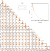 |
Fig. E.1 As Fig. D.1, but for 2M 0415 (single retrieval, with log g as a free parameter). |
| In the text | |
|
Fig. G.1 As Fig. D.1, but comparing the ultranest and PyMultiNest samplers for the HD 19467 B default retrieval. Both samplers used 1000 live points and ∆ ln Z = 0.5; ultranest with a slice sampler (nsteps = ndim = 30) and PyMultiNest with a constant sampling efficiency of 5%. This benchmark was run with an earlier setup than the final one, so the central values differ slightly from the adopted results quoted in the main text and Table C.1. |
| In the text | |
Current usage metrics show cumulative count of Article Views (full-text article views including HTML views, PDF and ePub downloads, according to the available data) and Abstracts Views on Vision4Press platform.
Data correspond to usage on the plateform after 2015. The current usage metrics is available 48-96 hours after online publication and is updated daily on week days.
Initial download of the metrics may take a while.