


| Issue |
A&A
Volume 710, June 2026
|
|
|---|---|---|
| Article Number | A164 | |
| Number of page(s) | 16 | |
| Section | Galactic structure, stellar clusters and populations | |
| DOI | https://doi.org/10.1051/0004-6361/202659278 | |
| Published online | 10 June 2026 | |
NGC 1647: A young open cluster with a broad main sequence observed with LAMOST
1
INAF – Osservatorio Astrofisico di Catania,
via S. Sofia, 78,
95123
Catania,
Italy
2
Institute for Frontiers in Astronomy and Astrophysics, Beijing Normal University,
Beijing
102206,
PR China
3
School of Physics and Astronomy, Beijing Normal University,
Beijing
100875,
PR China
4
Institut für Astronomie und Astrophysik, Eberhard Karls Universität Tübingen,
Sand 1,
72076
Tübingen,
Germany
5
INAF – Osservatorio di Astrofisica e Fisica dello Spazio,
via P. Gobetti 93/3,
40129
Bologna,
Italy
★ Corresponding authors: This email address is being protected from spambots. You need JavaScript enabled to view it.
; This email address is being protected from spambots. You need JavaScript enabled to view it.
Received:
2
February
2026
Accepted:
7
April
2026
Abstract
Aims. In this work we present the results of our analysis of medium-resolution LAMOST spectra of candidate members of the cluster NGC 1647 with the aim of determining the stellar parameters, activity level, lithium abundance, and to study the cluster properties.
Methods. We used the code ROTFIT to determine the atmospheric parameters (Teff, log g, and [Fe/H]), radial velocity (Vr), and projected rotation velocity (v sin i). Moreover, for solar-type and cooler stars (Teff≤ 6500 K), we calculated the Hα and Li Iλ6708 net equivalent width by means of the subtraction of non-active photospheric templates. We determined the rotation periods for 160 stars by analyzing the available TESS photometry.
Results. We derived Vr, v sin i, and atmospheric parameters for 341 spectra of 155 stars, plus three additional bright targets with archival UVES spectra. Moreover, we found four double-lined spectroscopic systems for which we provide the radial velocities of the two components. The Vr distribution of the cluster members peaks at −5.3 km s−1 with a dispersion of 1.6 km s−1, while the average metallicity is [Fe/H] = −0.08±0.08 dex, in line with previous determinations, which were based on only a handful stars. From the fitting of the spectral energy distribution of 160 likely members we infer the existence of a differential reddening across the cluster field with an average value of AV = 1.1 mag. The AV values show a distinct correlation with the color offset from the lower boundary of the main sequence, as observed in the Gaia color–magnitude diagram; conversely, this offset appears to be uncorrelated with v sin i. These two findings confirm that differential reddening is the primary driver behind the observed extended main-sequence turnoff (eMSTO) in this cluster. The age of NGC 1647, obtained from the lithium abundance, is 203±27 Myr, which is compatible with the values inferred from a gyrochronological approach and the isochrone fitting.
Key words: stars: abundances / stars: activity / binaries: spectroscopic / stars: fundamental parameters / open clusters and associations: individual: NGC 1647
© The Authors 2026
 Open Access article, published by EDP Sciences, under the terms of the Creative Commons Attribution License (https://creativecommons.org/licenses/by/4.0), which permits unrestricted use, distribution, and reproduction in any medium, provided the original work is properly cited.
This article is published in open access under the Subscribe to Open model. This email address is being protected from spambots. You need JavaScript enabled to view it. to support open access publication.
1 Introduction
The study of open star clusters (OCs) is fundamental for understanding the formation and evolution of the Galactic disk. Crucially, as groups of stars born simultaneously from the same progenitor cloud, OCs represent homogeneous samples in terms of both age and initial chemical composition (metallicity). This inherent uniformity makes them powerful tools for testing stellar evolutionary models, calibrating astrophysical distance scales, and mapping the chemical and structural properties of the Milky Way.
The advent of the Gaia mission has revolutionized cluster studies by providing highly accurate astrometric and photometric data for billions of stars. The extreme precision of these data has enabled an unprecedentedly complete census of cluster membership and allowed the definitive determination of cluster parameters, including distance, proper motion, and stellar density profiles. Recent efforts, notably by Cantat-Gaudin et al. (2018, 2020), and Hunt & Reffert (2024), have leveraged the massive Gaia datasets to redefine the membership and fundamental properties of thousands of OCs across the Galaxy.
The high photometric precision provided by Gaia also yields color–magnitude diagrams (CMDs) of exceptional detail. These CMDs reveal features such as the binary star sequence and the extended main-sequence turnoff (eMSTO) region of the main sequence (MS), the origin of which remains a subject of active debate in stellar astrophysics.
In this context, NGC 1647 serves as an excellent case study. Located in the Taurus-Auriga region, its CMD exhibits a broad MS (Zdanavičius et al. 2005). While the eMSTO phenomenon can contribute to this feature, the cluster’s position suggests that the observed broadness may be significantly influenced by differential extinction caused by intervening dust clouds in the Taurus region. NGC 1647 is a poorly studied cluster with only a few astrometric and photometric studies dating back several decades (e.g., Seares 1915; Geffert et al. 1996; Zdanavičius et al. 2005). More recently, NGC 1647 has been included in the large surveys that have automatically processed Gaia data (e.g., Cantat-Gaudin et al. 2020; Hunt & Reffert 2024). Both studies place the cluster at around 600 pc, but differ on its age (117–363 Myr) and extinction (AV=0.64–1.35 mag).
To address these issues and to derive better cluster parameters, such as the age and metallicity, spectra of a significant number of members in different regions of the CMD are needed. In this work, we conducted a comprehensive study of the cluster properties based on the characterization of the largest sample of members to date. By combining mid-resolution spectroscopy (R ≃ 7500) from LAMOST and Gaia DR3 astrometric and photometric data we delved deeper into the identification of the cluster members and their individual properties, such as atmospheric parameters, activity level, and lithium abundance. This allowed us to examine cluster properties and to investigate the origin of the observed eMSTO and broad MS.
This paper is structured as follows. Section 2 describes the selection of cluster members and the extraction of LAMOST mid-resolution data. Section 3 details the methodology used for the spectroscopic determination of stellar parameters and extinction. Section 4 presents the refined cluster properties, including the radial velocity distribution of the cluster members, a revised age, and metallicity. Section 5 discusses the implications of these findings, particularly in the context of the eMSTO and differential extinction. Finally, we summarize our conclusions in Sect. 6.
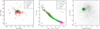 |
Fig. 1 Left panel: spatial distribution of the NGC 1647 members according to Hunt & Reffert (2024, magenta dots), Cantat-Gaudin et al. (2018, blue dots), and Qin et al. (2026, green dots). The symbol size scales with the G magnitude. The red circles highlight the data points that correspond to objects observed with LAMOST MRS. The black squares enclose the three stars with UVES archive observations. The meaning of the symbols is also indicated in the legend. Middle panel: color–magnitude diagram of the same sources. The arrow indicates the extinction vector for a value of AV = 1.1 mag. Right panel: proper motion diagram of all the Gaia DR3 sources with G ≤ 16 mag (small gray dots) in the field of NGC 1647 (center coordinates RA(2000) = 71.5◦, Dec(2000) = +19◦, radius=3◦). The cluster members are highlighted with the same symbols as in the other panels (red circles have been omitted to avoid confusion). The violet asterisk denotes the average proper motion of the cluster according to Hunt & Reffert (2024) and the violet ellipse is the 5σ contour. |
2 Observations and sample selection
2.1 Sample selection
To select the candidate members of this cluster, we used the catalog of Cantat-Gaudin et al. (2018), who listed 645 candidate members selected on the basis of Gaia DR2 astrometry and photometry (down to G = 18 mag) and the application of an unsupervised membership assignment code (UPMASK). Additionally, we used the new catalog of members of Galactic OCs compiled by Hunt & Reffert (2024), who used a similar approach, but with a different algorithm, namely the Hierarchical Density-Based Spatial Clustering of Applications with Noise (HDBSCAN) that was applied to the Gaia DR3 data down to magnitude G ≈ 20 mag. They found 982 members, 623 of which are in common with Cantat-Gaudin et al. (2018). The higher number of sources found by Hunt & Reffert (2024), apart from the different algorithm, is mostly the result of a larger sampled sky area and the deeper limiting magnitude.
A list of 931 candidate members was compiled by Qin et al. (2026) who also applied the HDBSCAN code to a sample of 40 070 Gaia sources selected around the center of NGC 1647 defined by Cantat-Gaudin et al. (2018) as explained in their work. In the latter sample, 764 objects overlap with the catalog presented by Hunt & Reffert (2024) and 614 objects overlap with that of Cantat-Gaudin et al. (2018). Furthermore, 610 stars are common to all three samples, which hereafter we refer to simply as the CG, H&R, and Qin samples. We considered this subset of 610 stars (henceforth the golden sample) to be bona fide candidates, electing not to use the membership probabilities, which are defined differently across the respective papers.
2.2 LAMOST spectroscopy
Following a five-year low-resolution spectroscopic survey (LRS; RLRS ≃ 1800, λ ∈ [3000,9000] Å, Zhao et al. 2012; Luo et al. 2015), LAMOST launched its medium-resolution spectroscopic survey (MRS; RMRS ≃ 7500) in September 2017 (Liu et al. 2020). The MRS covers the λ ∈ [4950,5350] Å (blue) and λ ∈ [6300,6800] Å (red) bands.
In this work, we utilized LAMOST MRS DR121, which comprises about 46 million spectra collected through June 2023. This data release is presently restricted to the Chinese astronomical community. The cross-match of our sample of members with the LAMOST DR12 catalog, adopting a radius of 3.″7 on the basis of the fiber pointing precision (0.″4) and the 3.″3 diameter of the fiber (e.g., Zong et al. 2018), produced 173 targets with a total of 428 MRS spectra, 159 of which have spectra with a sufficient signal-to-noise ratio (S/N typically ≥5) in at least one arm that we considered worthy to be analyzed (red circles in Fig. 1). In total we analyzed 345 LAMOST MRS co-added spectra corresponding to 159 candidate members of NGC 1647, 114 of which are in the golden sample of bona fide members, while 45 of them belong to two (or only one) of the C-G, H&R, and Qin samples and are thus considered lower-probability members. To estimate the potential contamination of the golden sample, we cross-checked the membership probabilities (P) from the three reference catalogs. Out of the 114 golden sample sources, 113 (99%) have a membership probability P > 0.5 in at least one catalog, while 80 sources (70%) meet the more stringent criterion of P > 0.5 in all three catalogs simultaneously. This indicates that the fraction of potential nonmembers is negligible (less than 1%) under a relaxed threshold and remains well-constrained at ≈30% even when adopting the most restrictive membership criteria. We chose to use co-added spectra, where each spectrum is the sum of all exposures obtained during a single observing night, to achieve the best possible S/N.
A precise evaluation of the spectral resolution, Rλ, during the observations of our targets is a necessary prerequisite to the subsequent analysis, especially for correctly measuring rotational broadening. To achieve this, we used the spectra of Th-Ar calibration lamps acquired during the science observations. For both arms we found values larger than the nominal Rλ = 7500: specifically, Rblue = 8200 ± 200 and Rred = 8400 ± 300. More details can be found in Appendix A.
2.3 Archive spectra
Since the LAMOST spectra do not cover the brightest MS targets, which are critical for constraining the eMSTO and the cluster age, we supplemented our dataset with archival data. We retrieved high-resolution spectra for three such stars: HD 30123, HD 284839, and HD 284841. These spectra were originally collected in February 2019 by Siebenmorgen et al. (2020), under ESO program 0102.C-0040, with UVES at the VLT-U2 telescope, using the CD#2 and CD#4 cross-dispersers and resolutions of about 65 000 and 74 500 for the blue and red arm, respectively. The aim of these observations was to investigate interstellar clouds. While Fitzpatrick & Massa (2007) classified these targets as B8 III or B9 III, Siebenmorgen et al. (2020) assigned spectral types in the range B5–B8 and luminosity class V or IV. Notably, HD 30123, the second brightest MS star in the cluster, is identified as a Be star, exhibiting distinct core emission in both Balmer and Paschen lines. We used these spectra for determining the atmospheric parameters and radial and rotational velocities as for the stars with LAMOST data.
2.4 Photometry
Time-series photometric observations form the foundation for studying stellar rotation periods. In NGC 1647, a total of 112 members were observed by the K2 mission (Howell et al. 2014; Furlan et al. 2018). However, because all stars with K2 light curves also have observations from the Transiting Exoplanet Survey Satellite (TESS; Ricker et al. 2015), and since our primary goal was to determine reliable rotation periods for the largest number of targets as possible, we based our analysis exclusively on the TESS photometry. In total, 623 candidate members possess TESS light curves. All of them were observed in Sectors 43 (September 16 to October 11, 2021) and 44 (October 12 to November 5, 2021), providing nearly continuous, high-quality photometry over approximately 55 days with a cadence of 600 s. A subset of stars also received additional monitoring in Sectors 70 (September 20 to October 16, 2023) and 71 (October 16 to November 11, 2023), where the exposure time was 200 s. These additional data extend the observational baseline and enable independent confirmation of rotational signals when present. We retrieved the TESS Science Processing Operations Center (SPOC) light curves (Caldwell et al. 2020) available in the Mikulski Archive for Space Telescopes (MAST)2 through the Lightkurve package (Lightkurve Collaboration et al. 2018). The latter was also used for a quick look and data preparation for the following analysis, which was based on the Pre-search Data Conditioning Simple Aperture Photometry (PSDCSAP).
3 Data analysis
The code ROTFIT (e.g., Frasca et al. 2006, 2015) was used to measure Vr, v sin i, and the atmospheric parameters (Teff, log g, and [Fe/H]). The version of ROTFIT developed for LAMOST MRS was described by Frasca et al. (2022), who analyzed thousands of MRS spectra in the Kepler field, and by Frasca et al. (2025), who applied it to the MRS spectra of the Pleiades cluster members. For objects cooler than about 7000 K (henceforth cool stars), as judged from the spectrum appearance and the position on the CMD, ELODIE archive spectra (R ≃ 42 000; Moultaka et al. 2004) of slowly rotating stars (v sin i ≤ 3 km s−1) with a low activity level (based on the residual flux in the Hα core) were used as templates. This grid is composed of spectra of 388 different stars of FGKM spectral types (Teff ≤ 7000 K), which sufficiently cover the space of parameters, especially at metallicity values around [Fe/H]=0 dex. For stars hotter than or close to 7000 K (hereafter hot stars), we used instead a grid composed of synthetic BT-Settl spectra (Allard 2014) with a solar metallicity, Teff in the range 6000–12 000 K, and log g between 3.0 and 5.0 (in steps of 0.5 dex). As the grid of the spectra is computed with steps of [Fe/H] = 0.5 dex, we used the value of [Fe/H]=0 dex, which is the closest to the previously derived cluster metallicity. These stars are located in the Gaia CMD at a G ≤ 12.9 mag and GBP − GRP color bluer than 1.12 mag. For a few stars close to the threshold for hot stars we used both template grids to check the consistency of the results. An example of the fitting results by the ROTFIT code with both template grids is shown in Fig. B.1. For the cool stars we opted for real-star templates, because they reproduce more faithfully the photospheric features and they are best suited for the measure of Hα chromospheric core emission and the Li I absorption by the application photospheric spectral subtraction.
For the stars with more LAMOST MRS spectra we computed, for each arm, the atmospheric parameters for all the spectra (excluding those with strong flaws) and averaged them using a variance-defined weight  , where σi is the error of the given parameter in the i-th measure. Therefore, we obtained two sets of parameters per each star, one derived from the analysis of the blue-arm and the other of the red-arm spectra. The comparison of the results from the two arms was used to evaluate the accuracy of our measures in different regions of the parameter space (Sects. 3.1 and 3.2). The final parameters, which are reported in Table 1, are the weighted mean of the values derived from each arm, using the variance-defined weights, as before. The uncertainties for the parameters listed in Table 1 represent the maximum value between the standard error of the weighted mean and the weighted standard deviation derived from the measurements obtained from the blue- and red-arm spectra.
We analyzed the three archival UVES spectra using a spectral-synthesis approach, since the combination of high effective temperature and rapid rotation results in a severe paucity of measurable metal lines. The synthetic spectra were computed in three steps. First, LTE model atmospheres were calculated with the ATLAS9 code (Kurucz 1993). Second, the corresponding synthetic spectra were generated with the radiative-transfer code SYNTHE (Kurucz & Avrett 1981). Third, the best-fitting solution was obtained with ad hoc IDL routines by minimizing the χ2 of the residuals between observed and synthetic spectra. The stellar parameters Teff and log g were primarily constrained from the Balmer-line profiles in the blue UVES arm. The projected rotational velocity, v sin i, was determined by fitting the Mg II λ4481 Å line, and all synthetic spectra were convolved with the instrumental line-spread function (set by the UVES resolving power) and with the rotational broadening kernel before comparison with the observations. Owing to the small number of iron lines and the strong rotational broadening, the metallicity could not be inferred. Therefore, we fixed it to [Fe/H] = 0 dex, consistently with the assumption adopted for the hot LAMOST sources.
Stellar parameters of the investigated sources (extract).
3.1 Radial velocity
The radial velocities measured on LAMOST MRS spectra are affected by systematic offsets in different runs that are related to the wavelength calibration and are different for the blue and red arm of each spectrograph (e.g., Zong et al. 2020; Frasca et al. 2022). To correct for the radial velocity zero-point offsets, we cross-matched our sample with the official LAMOST DR 12 catalog and adopted the corresponding zero-point corrections for the red and blue arms provided therein. For spectra without available correction parameters (i.e., those with default values of −9999 in the LAMOST DR12 catalog), we applied the typical offsets reported by Wang et al. (2019), namely +0.25 km s−1 for the blue arm and −0.09 km s−1 for the red arm.
The Vr uncertainties derived from ROTFIT and reported in Table 1 range from 0.4 to 27.3 km s−1, with a median value of 2.2 km s−1. To investigate the precision of the Vr measures and its dependence on other parameters, such as the v sin i, we compared the results of the blue- and red-arm spectra, which are obtained simultaneously. This comparison is shown in Fig. 2, where we used a symbol size proportional to v sin i and different colors for the hot and cool stars that were analyzed with different grids of templates, as explained in Sect. 3. The largest scatter around the one-to-one relation is displayed by the fastest rotators, which are mostly hot stars. The root-mean-square (rms) of the difference  is about 6.9 km s−1, which reduces to about 3.6 km s−1 if we exclude the stars with v sin i ≥ 70 km s−1. By dividing this value by
  , as it includes the uncertainties of the Vr in the two arms, we get an estimate of 2.5 km s−1 for the average precision of the Vr measurements, which is close to that found by us for the LAMOST MRS observations of the Pleiades (Frasca et al. 2025).
We performed a search for sources displaying intrinsic radial velocity variability – indicative of binarity or pulsations – by analyzing objects for which multiple spectra were acquired on separate nights. To identify statistically significant variations, we computed the reduced χ2 statistic and the corresponding probability P(χ2) that the Vr scatter is merely due to random chance (e.g., Press et al. 1992). We assigned the RVvar flag in Table 1 to the 31 sources where P(χ2) < 0.05, indicating significant Vr variation. For these candidates, we have between two and five spectra per source, with a median of three. We found no objects previously classified as single-lined spectroscopic binaries (SB1s) in our sample, with the exception of Gaia DR3 3409916343231260032, which is classified as an SB1 in the Gaia DR3, nonsingle stars catalog (Gaia Collaboration 2023). However, this source was not analyzed by us for the atmospheric parameters, due to the low S/N of the single LAMOST MRS spectrum we possess. The Vr derived from the blue arm, −25.6 ± 1.7 km s−1, is significantly different from the cluster average, as expected for an SB1 system. Furthermore, for four objects (five spectra in total), we observed two CCF peaks above the noise that were deemed significant. These objects were classified as new double-lined spectroscopic binaries (SB2s). Since the parameters derived for these objects are unreliable, they are not included in Table 1; instead, we report the measured Vr values for both components of these new SB2s in Table B.1, where Vr1 corresponds to the component with the highest CCF peak.
For a quality check, we compared in Fig. B.2 the average Vr values of the single-lined sources (Table 1) with those contained in the Gaia DR3 catalog, which were derived using the RVS spectrograph. Many targets follow a one-to-one relation and cluster around the mean radial velocity of NGC 1647, with some sources, including a few among those classified by us as ‘RVvar’, exhibiting significant scatter.
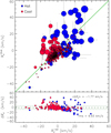 |
Fig. 2 Comparison between the radial velocities measured from blue-and red-arm LAMOST MRS spectra (top panel). Blue and red symbols are used for the hot and cool stars, analyzed with BT-Settl and ELODIE grids of templates, respectively. The symbol size scales with the v sin i of the source. The one-to-one relation is shown by the solid green line. The differences |

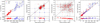 |
Fig. 3 Comparison of the atmospheric parameters derived from the blue- and red-arm LAMOST MRS spectra using ROTFIT. The panels, from left to right, show the effective temperature (Teff), surface gravity (log g), metallicity ([Fe/H]), and projected rotation velocity (v sin i). The symbols are consistent with those presented in Fig. 2. We note the significantly larger rms dispersion observed for the Teff of the hot stars (blue data points). |
3.2 Atmospheric parameters and projected rotation velocity
Comparing the blue- and red-arm values for the other stellar parameters (Teff, log g, [Fe/H], and v sin i) allows us to obtain reliable estimates of their errors in different regions of the parameter space and to highlight any specific issues encountered during their determination (Fig. 3). As explained previously, we generated two sets of parameters for each source – one from the analysis of the blue-arm spectrum and one from the red-arm spectrum – which we can compare, as we did for the radial velocities.
Regarding the effective temperature, the measured values generally follow the one-to-one relation, although a significantly larger scatter is apparent for the hot stars compared to the cool ones. This is likely due to the characteristics of early-type spectra, which feature fewer and shallower absorption lines, particularly in the red spectral range, combined with higher average v sin i values that further blend the available diagnostic features. Specifically, the average difference between blue-arm and red-arm effective temperature is  for the cool stars and −162 K for the hot stars. The rms deviation is ≈250 K for the cool stars, while it increases to about 850 K for the hot ones. This larger dispersion for the hot targets is consistent with the average errors evaluated by ROTFIT, which scale with the Teff, yielding median values of 55 K for the cool stars and 210 K for the hot ones.
The remaining parameters (log g, [Fe/H], and v sin i) exhibit very good agreement for the cool spectra (ELODIE templates) between the two independent arm analyses, with very small average offsets and rms dispersions of approximately 0.15 dex, 0.18 dex, and 23 km s−1, respectively. For the hot stars, the gravity values are clustered around the available model steps (log g=3.5 dex, 4.0 dex, and 4.5 dex). Furthermore, the single data point observed in the [Fe/H] plot is a direct result of our choice to use only solar metallicity BT-Settl spectra.
The scatter on v sin i is significantly reduced for sources with v sin i < 100 km s−1, dropping to about 15 km s−1. Notably, the v sin i measurements appear equally robust for both hot and cool spectra, as illustrated in the right panel of Fig. 3 and confirmed by a similar overall rms scatter (≈30 km s−1). As previously reported by Frasca et al. (2022), the resolution and sampling of the LAMOST MRS spectra prevent reliable measurements of v sin i values below 8 km s−1. Therefore, any measurement smaller than this limit in at least one arm must be considered a non-detection. Accordingly, we treated the final v sin i values (the weighted averages of the blue and red arms) that are less than 8 km s−1 as upper limits and flagged them appropriately in Table 1.
A statistically significant comparison between the parameters measured by us using the LAMOST MRS spectra and values available in the literature, which could serve as a quality control for our data, cannot be performed. In fact, there are only seven stars observed within the GALactic Archaeology with HERMES (GALAH) Survey (Buder et al. 2021) and six stars observed by APOGEE (Abdurro’uf et al. 2022) that overlap with those observed by LAMOST MRS; the majority of these are cool objects. The temperature values for these few overlapping sources show a substantially good agreement (rms = 337 K, excluding the three hot sources observed by APOGEE). As regards the metallicity, the values from the literature are scattered around [Fe/H] = 0 dex with a dispersion much larger than our values.
Accurate parameter values were derived by Carrera et al. (2022) for the only two giant stars in the cluster using high-resolution spectra, but we do not possess LAMOST MRS spectra for these sources. Nonetheless, the parameters derived from those high-resolution data by Carrera et al. (2022) have been utilized in the subsequent analysis.
4 Results
4.1 Radial velocity distribution
We have Vr values for 158 single-lined sources (including the three MS stars with UVES spectra). For each of those with multiple LAMOST observations we calculated the weighted average of the individual values (with  as the weight), which are also reported in Table 1 along with the error, which is the largest between the standard error and the weighted standard deviation of individual values. With these average radial velocities, we built the Vr distribution, which is shown as a green histogram in Fig. 4. The center µ = −5.18 km s−1 and the dispersion σ = 1.65 km s−1 of this distribution were found by means of a Gaussian fitting. We note that the intrinsic dispersion of the cluster RV distribution is narrower than the median formal uncertainty derived from ROTFIT (≈2.2 km s−1). This suggests that our formal error estimates are likely conservative, particularly for stars with high signal-to-noise spectra and low rotation.
Since a relevant fraction of the selected candidates is composed of warm (Teff ≥ 7000 K) and fast rotating stars, we distinguished the slowly (v sin i ≤ 70 km s−1) and the fast rotating (v sin i > 70 km s−1) stars, for which the measure of Vr is less accurate. We have overplotted their Vr distributions with different colors in Fig. 4. As apparent, the fast rotating stars display a flatter and more scattered distribution compared to the slowly rotating ones. The distribution of the latter subsample (94 sources) is similar to that of the full sample and is fitted by a Gaussian with µ = −5.32 km s−1 and σ = 1.57 km s−1. We consider the latter values as more representative for the average Vr of the cluster and its dispersion, although the inclusion of the fast-rotating stars does not significantly affect the result.
Some of the values significantly far from the Gaussian center (by more than 5σ) may be partially attributed to single-lined spectroscopic binaries (SB1s) or pulsating stars. In Fig. 4, we highlight potential SB1 systems (those labeled as RVvar in Table 1) whose average radial velocity falls within this range using orange dots. The extended tail of the Vr distribution may also be attributed to nonmember contaminants or a stellar population characterized by a more dispersed kinematic distribution. Notably, this tail contains numerous stars excluded from the golden sample of high-probability members; these objects are highlighted with blue downward arrows in Fig. 4.
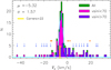 |
Fig. 4 Radial velocity distribution obtained from all analyzed LAMOST MRS spectra of the cluster members (green histogram). Separate distributions are shown for the slowly rotating and fast rotating stars, as indicated in the legend. The best-fit Gaussian function applied specifically to the slowly rotating stars histogram is overplotted as a solid cyan line; its center (µ) and dispersion (σ) are also marked. The cluster Vr measured by Carrera et al. (2022) is indicated by the vertical yellow bar. The downward blue arrows highlight lower-probability targets (those not included in the golden sample) that lie outside the 5σ limit of the Gaussian center. Within this same velocity range, the orange dots denote the mean Vr of sources exhibiting variable radial velocity. |
4.2 Cluster metallicity
Similar to the other parameters, the final metallicity listed in Table 1 is the weighted average of the values derived from the blue and red arms. The [Fe/H] distribution for the cool stars is shown in Fig. 5, distinguishing the stars in the golden sample with a different color histogram. However, the two distributions are basically the same and are both centered at slightly under-solar values. By fitting them with a Gaussian, we derive an average cluster metallicity of [Fe/H] = −0.12 ± 0.11 dex, where the Gaussian dispersion (σ) is taken as the cluster metallicity uncertainty. If we calculate instead the weighted average and standard deviation of the metallicity values we find <[Fe/H]>= −0.08 ± 0.08 dex for both the full and golden sample. These values are in good agreement with the robust metallicity determination made by Carrera et al. (2022) for the two giant member stars, which was based on high-resolution spectra.
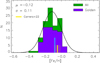 |
Fig. 5 Metallicity ([Fe/H]) distribution for all the cool stars of NGC 1647 (green histogram) and for the high-probability golden sample (purple histogram). The best-fit Gaussian function is overlaid as a solid black line; its center (µ) and dispersion (σ) are also marked. The cyan line denotes the weighted average of our [Fe/H] measures. The weighted-average metallicity measured by Carrera et al. (2022) for the two giants of the cluster is indicated by the vertical yellow bar, with the associated uncertainty represented by the hatched histogram. |
4.3 SED Fitting: reddening and luminosities
To determine the interstellar extinction (AV) and luminosity (L) for our sources, we employed the spectral energy distribution (SED) fitting method. We constructed the corresponding SEDs using publicly available optical and NIR photometric data and fitted them with BT-Settl synthetic spectra (Allard 2014). Specifically, for the majority of sources, we utilized optical BVg′r′i′ photometry from the APASS catalog (Henden et al. 2016) and NIR data from 2MASS (Skrutskie et al. 2006). Additionally, mid-infrared data from the WISE catalog (Cutri et al. 2021) were retrieved to identify potential mid-IR excesses and for visualization purposes. These data were excluded from the actual SED fit, which was restricted to the BVg′r′i′JHKs bands. No sources exhibiting mid-IR excess were found. For the few sources lacking APASS entries, we substituted the optical data with Sloan photometry from the Pan-STARRS catalog (Magnier et al. 2020).
For each target, we fixed the distance using its Gaia DR3 parallax and adopted the atmospheric parameters (Teff and log g) derived in Sect. 3. We included the two giants, whose parameters were measured by Carrera et al. (2022). This fitting method left the stellar radius (R) and AV as free parameters. These variables were determined via χ2 minimization, and the stellar luminosity was subsequently calculated as  . Two examples of the fitting procedure for a hot and a cool stars are presented in Figs. B.3 and B.4, respectively. Uncertainties for AV and R were derived from the 1σ confidence level of the χ2 maps. To account for the Teff–AV degeneracy, we incorporated the uncertainty in Teff by recalculating the best-fit values at its upper and lower 1σ limits.
The AV values determined by us via the SED fitting of the 160 sources with known parameters (including the three MS stars with UVES spectra and the two giants) range from about 0.3 to 2.1 mag and are reported in Table B.2. The AV distribution is displayed in Fig. 6 along with that of the AV values measured by Zdanavičius et al. (2005), which span the same range. The weighted average extinction from our measures is AV=1.12 ± 0.30 mag, where the error represents the weighted standard deviation. The same average value, AV=1.10 ± 0.33 mag, is found from the photometric determination by Zdanavičius et al. (2005). Assuming a standard reddening law with RV=3.1, this corresponds to E(B − V) = 0.35 ± 0.11 mag. For 43 sources we have AV measured both in this work and from Zdanavičius et al. (2005). As shown in Fig. B.5, these AV values are well correlated with each other, with a Pearson’s correlation coefficient ρ = 0.677. This reinforces the validity of our analysis.
As a further test of the reliability of our extinction measurements, we have overlaid the stellar positions in Fig. 7 on an IRAS 100 µm emission map, displayed in grayscale with inverted intensity levels. This map effectively traces the dust column density along the line of sight. The symbols are color-coded by extinction value, demonstrating a strong spatial correlation between the measured AV and the 100 µm thermal emission.
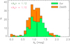 |
Fig. 6 Extinction distribution for all the NGC 1647 members with LAMOST data (green histogram) and for the stars analyzed by Zdanavičius et al. (2005) (Zda05, orange histogram). The average AV values from the two datasets are marked with vertical solid lines and are reported in the corresponding color in the upper left corner of the panel. |
4.4 Hertzsprung-Russell diagram
An additional tool used to validate our results and infer the cluster age is the Hertzsprung-Russell diagram, presented in Fig. 8 alongside PARSEC isochrones (Nguyen et al. 2022) for [Fe/H] = −0.08 dex at four different ages. This diagram plots intrinsic (unreddened) quantities, as extinction was accounted for during the luminosity calculations.
As shown in the figure, most targets are located in the region where the MS isochrones overlap; consequently, the MS targets observed with LAMOST MRS alone provide limited constraints on the cluster age. In this regard, the parameters of the two giants and the bright MS stars observed with UVES are particularly useful. Their positions in the Hertzsprung-Russell diagram allow us to exclude ages significantly younger than 150 Myr or older than 200 Myr. This age range is consistent with both previous determinations and the age inferred by us from the lithium depletion pattern (see Sect. 4.5). Furthermore, this result is in good agreement with the asteroseismic age derived by Qin et al. (2026).
In Fig. 8, we have enclosed in green squares the stars marked with blue arrows in Fig. 4. These represent objects that do not belong to the golden sample and have Vr deviating by more than 5σ from the cluster mean (−5.32 km s−1). The most striking case is Gaia DR3 3406926251422646400, which lies well above the MS and is identified as a subgiant (K0 IV, Teff = 5153 K, and log g = 3.53 dex) unrelated to the cluster.
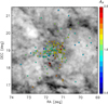 |
Fig. 7 Spatial distribution of the stars in our sample. The symbols are color-coded according to their individual AV values. The grayscale image in the background is the 100 µm IRAS flux map. |
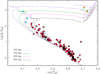 |
Fig. 8 HR diagram for NGC 1647. The MS stars are denoted with dots (red for LAMOST MRS and cyan for UVES spectra). The orange squares represent the two giants studied by Carrera et al. (2022). PARSEC isochrones (Nguyen et al. 2022) at 100, 150, 200, and 300 Myr for models with the cluster metallicity ([Fe/H] = −0.08 dex) are overlaid. Green squares enclose the lower-probability members indicated by arrows in Fig. 4. |
4.5 Chromospheric emission and lithium abundance
For stars later than about F5 spectral type, both chromospheric emission (traced by the Balmer Hα line in the LAMOST MRS spectra) and lithium absorption are age-dependent parameters (see, e.g., Jeffries 2014; Frasca et al. 2018, and references therein). Since chromospheric emission in Hα can only show up as a small filling of the line core, which depends on the star’s activity level and photospheric flux, removal of the underlying photospheric spectrum is mandatory. To achieve this, we subtracted a non-active, lithium-poor template spectrum that best matches the final atmospheric parameters from each LAMOST red-arm spectrum. This template was aligned to the Vr of the target, rotationally broadened by convolution with a rotational profile corresponding to the measured v sin i, and resampled onto the spectral points of the target spectrum.
The emission Hα equivalent width  was then measured by integrating the residual emission profile, as also shown in Frasca et al. (2022). We adopted the convention of
  for excess emission. We excluded the SB2 systems from this analysis and retained only the
  values that were significantly larger than zero – that is, those greater than or equal to their respective errors (70 sources). For the remaining 15 single-lined sources, the error was adopted as the upper limit of the measurement. These data are reported in Table 2, where we list the weighted mean of the values measured in the individual spectra for stars with multiple observations. The equivalent width of a chromospheric line is generally not the optimal diagnostic for magnetic activity. More accurate indicators of chromospheric activity are the line flux in units of stellar surface
  and the ratio between the line luminosity and bolometric luminosity
  . These values were evaluated according to Eqs. (2) and (3) of Frasca et al. (2022) and are also reported in Table 2.
The Hα luminosity ratio,  , is plotted as a function of Teff in Fig. 9. This plot also displays the dividing line, empirically determined by Frasca et al. (2015), which separates chromospherically active stars from objects still undergoing mass accretion. This line is situated close to the level of saturated chromospheric activity, defined as
  by Barrado y Navascués & Martín (2003). The
  values measured in our study place all NGC 1647 members firmly within the region of chromospherically active sources, largely occupying the same domain as the Pleiades members (Frasca et al. 2025). The only apparent difference between the two clusters in this diagram is the lack of MS stars cooler than about 5200 K for NGC 1647. This is the results of the larger distance and extinction of NGC 1647, which limits our ability to observe these fainter, cooler stars. This prevents us from studying the saturated regime in this cluster, as we did in Frasca et al. (2025), and to use this diagram as an age proxy.
The equivalent width of the Li I λ6708 Å absorption line (EWLi, defined as positive for absortpion) was also measured in the residual (subtracted) spectra, where blends with nearby photospheric lines had effectively been removed. This procedure ensures a better measure of EWLi and a reliable estimate of its error. The error was calculated as  , where D is the average dispersion of the flux values in the residual spectrum on both sides of the line (with
  ), w is the integration width in wavelength units, and ∆λ (=0.15 Å) is the pixel size in wavelength units. This expression is consistent with the formula proposed by Cayrel (1988).
We successfully detected the lithium line ( in at least one spectrum) for 85 objects, while for 2 objects we could only determine an upper limit. We did not measure EWLi for the SB2 systems. For stars with time-series spectra, we calculated the weighted mean of the individual EWLi values and adopted the weighted standard deviation or the standard error of the weighted mean (whichever was greater) as the error estimate. For objects with only non-detections across all their spectra, we adopted the lowest upper limit. These final values are quoted in Table 3.
Lithium is a fragile element that is burned in stellar interiors at temperatures as low as 2.5×10⁶ K. It is progressively depleted from the stellar atmosphere as internal mixing reaches the Li-burning layer, with the depletion rate dependent on the star’s internal structure (i.e., stellar mass). Consequently, Li abundance serves as a robust age proxy for stars cooler than about 6500 K. We derived the lithium abundance, A(Li), from our values of Teff, log g, and EWLi by interpolating the curves of growth presented by Lind et al. (2009). These curves span the Teff range 4000–8000 K and log g from 1.0 to 5.0 dex and include corrections for non-LTE effects. The errors of A(Li) were calculated by propagating the uncertainties in Teff and EWLi. These final abundances are listed in Table 3.
Notes. The full table is available at the CDS. (a) LAMOST designation. (b) Subsample to which the target belongs.
On the basis of the Teff (Sect. 3.2) and EWLi measurements, we estimated the cluster age by using the EAGLES code (Jeffries et al. 2023). This code fits Li-depletion isochrones to the Teff (in the range 3000–6500 K) and EWLi values of a coeval stellar group. We note that EAGLES performs optimally for clusters exhibiting a wide Teff distribution among their members, reaching out the coldest members, where the Lithium depletion is more pronounced. Unlike nearby clusters, like the Pleiades (e.g., Frasca et al. 2025), the useful LAMOST MRS spectra of the NGC 1647 members are limited to stars as cool as the Sun, with only a handful of stars extending down to ≈5300 K. However, this temperature range is sufficient to obtain a reliable estimate of the age of NGC 1647. For this analysis, we selected the stars cooler than 6500 K, including also the few EWLi upper limits (a total of 73 objects). The results of applying EAGLES to our data are shown in Fig. 10. We find an age of 203 ± 27 Myr.
Activity indicators: Net Hα equivalent width  , line flux
  , and luminosity ratio
  (extract).
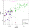 |
Fig. 9 Hα luminosity ratio |


Lithium equivalent widths (EWLi) and abundances (A(Li)) (extract).
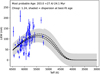 |
Fig. 10 Fit to the lithium depletion pattern of the EWLi measured in this work obtained with the EAGLES code (Jeffries et al. 2023). |
4.6 Gyrochronology
Another helpful diagnostic tool for cluster age estimation is the distribution of rotation periods when plotted against stellar mass or a color index (e.g., Barnes 2003, and references therein). To this end, as mentioned in Sect. 2.4, we used the high-precision, high-cadence photometric TESS data to measure the rotation period for the largest possible number of cluster members. In total, we analyzed the light curves of 637 members of NGC 1647 by means of a Lomb–Scargle periodogram to search for the highest frequencies in their power spectra. We focused on the low-frequency domain of the power spectrum ( f ≤ 10 d−1), which contains the power excesses typically associated with rotational modulations caused by starspots on the stellar photospheres. For each star, we visually inspected the periodogram and the phase-folded light curve. By combining the periodic signals with the stars’ effective temperatures, surface gravities, and their locations on the CMD, we identified a sample of 160 stars whose variability is confidently attributed to stellar rotation. These stars occupy the lower main sequence and exhibit a single, well-defined peak in the periodogram, characteristic of spot-induced rotational modulation. The uncertainties in Prot were conservatively estimated from the half-width at half-maximum of the corresponding periodogram peak and are reported alongside the periods in Table B.3.
We compared the rotation periods derived in this work with those reported by Long et al. (2023). We identified 15 stars in common between the two samples, and their rotation periods show excellent agreement, as can be seen in Table B.4. Furthermore, when comparing our results with those from Breton et al. (2025), we found two overlapping sources whose rotation periods are also fully consistent.
We applied extinction corrections to obtain homogeneous intrinsic colors. Since our goal is to compare NGC 1647 with other benchmark OCs, whose members have Gaia magnitudes and colors, we did not adopt the extinction AV values derived from our SED fitting. Instead, we used the machine-learning regression extinction map from Bai et al. (2020), which provides uniform estimates of Gaia color excess E(GBP − GRP) across the sky. The intrinsic color for each star was therefore computed as

After obtaining the de-reddened colors, we then constructed the color-period diagram (CPD) for NGC 1647 using the de-reddened (GBP − GRP)0 colors and the derived rotation periods. The results are shown as black crosses in Fig. 11. For comparison, we overplotted the rotation sequences of two benchmark clusters: the 125 Myr Pleiades (orange points, Rebull et al. 2016; Frasca et al. 2025) and the 300 Myr NGC 3532 (blue points, Barnes 2003; Fritzewski et al. 2021). The rotation-period distribution of NGC 1647 falls between these two reference clusters. In particular, its upper I sequence (slow rotators) overlaps that of the Pleiades and the low-color portion of that of NGC 3532, lying in between the two ones. Its lower C sequence (fast rotators) is more similar to that of the Pleiades, because fast rotators are observed only for low-mass stars, (GBP − GRP)0 > 1.1, in 300-Myr-old clusters like NGC 3532, and the C sequence totally disappears at older ages. This comparison indicates that NGC 1647 has an intermediate level of rotational evolution. Therefore, based on gyrochronology, we infer that the age of NGC 1647 lies between approximately 125 and 300 Myr, in good agreement with the constraints from CMD isochrone fitting and photospheric lithium abundances.
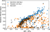 |
Fig. 11 Rotation periods vs. the dereddened color index (GBP − GRP)0 for the members of NGC 1647 (black crosses). The periods of Pleiades (τ ≃ 125 Myr) members based on K2 (Rebull et al. 2016) and TESS (Frasca et al. 2025) are overplotted as orange dots, while those of NGC 3532 (τ ≃ 300 Myr) members (Fritzewski et al. 2021) are shown as blue dots for comparison. |
5 Discussion
The phenomenon of eMSTO was first detected in massive Mag-ellanic Cloud clusters and initially interpreted as a manifestation of prolonged star formation lasting several hundred million years (e.g., Milone et al. 2009). More recently, eMSTOs and broadened main sequences have been identified within Galactic OCs (e.g., Cordoni et al. 2018, 2024, and references therein). However, no direct evidence of such long-lived star formation has been found (e.g., Cabrera-Ziri et al. 2016). Moreover, many low-mass OCs lack the escape velocity required to retain the gas necessary for secondary star-forming events (Bastian et al. 2018).
The most widely accepted explanation currently attributes the eMSTO to a spread in stellar rotation rates among stars of the same age (Bastian & de Mink 2009; Lim et al. 2019). Rapid rotation causes structural changes (centrifugal support) and internal mixing, making these stars appear cooler (redder) and extending their main-sequence lifetimes. Furthermore, for very fast rotators, the inclination of the rotation axis plays a significant role: due to gravity darkening, the stellar poles appear hotter and brighter than the equatorial regions, making the observed color and magnitude dependent on the viewing angle. In specific cases, such as the cluster Stock 2, the observed eMSTO is primarily caused by non-uniform interstellar extinction (differential reddening) rather than intrinsic stellar physics (Alonso-Santiago et al. 2021). However, this does not appear to be a universal cause, as many clusters with eMSTOs show no significant reddening variations (Cordoni et al. 2018).
To investigate the primary mechanism driving the eMSTO and the broadened MS in NGC 1647, we examined potential correlations between a star’s position on the Gaia CMD and parameters such as stellar rotation and extinction. Operationally, we empirically defined a lower envelope for the MS belt (see Fig. B.6) using a fourth-order polynomial and calculated the color offset of each star relative to this locus. In Fig. 12 we plot v sin i values against the observed color offset. As evidenced by the figure, and further supported by a near-zero Pearson correlation coefficient (ρ = 0.015), stellar rotation does not appear to be the primary mechanism driving the MS broadening. In contrast, Fig. 13 illustrates that interstellar extinction exhibits a strong correlation with the Gaia color shift. We find Pearson correlation coefficients of 0.520 using our AV estimates and 0.722 using the AV values from Zdanavičius et al. (2005). This provides compelling evidence that differential extinction accounts for most, if not all, of the observed MS spread.
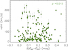 |
Fig. 12 Projected rotational velocity (v sin i) vs. the Gaia color shift ∆(GBP −GRP). The color shift is measured relative to the lower envelope of the MS strip (Fig. B.6). The Pearson’s correlation coefficients (ρ) is marked in the upper right corner of the panel. |
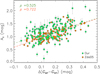 |
Fig. 13 Extinction (AV) vs. the Gaia color shift ∆(GBP − GRP). The data derived in the present work and by Zdanavičius et al. (2005) are distinguished by different colors, as indicated in the legend. The linear best fits to our data and to the Zdanavičius et al. (2005) data are shown as a green dashed line and an orange dot-dashed line, respectively. The Pearson’s correlation coefficients (ρ) are also marked in the upper left corner. |
6 Summary
We have presented the results of the analysis of 347 LAMOST medium-resolution spectra of stars that are members or candidates to the NGC 1647 open cluster. This represents by far the largest sample studied to date. We were able to determine, with the analysis code ROTFIT, the atmospheric parameters (Teff, log g, and [Fe/H]), the radial velocity (Vr), and the projected rotational velocity (v sin i) for most of these spectra corresponding to 158 unique stars. For four additional sources that we discovered as new double-lined spectroscopic binaries (SB2s), we report the radial velocities of the two components but did not determine their parameters.
We found a radial velocity distribution with a nearly symmetric peak centered at −5.32 km s−1 with a dispersion σ = 1.57 km s−1. Some discrepant Vr values (by more than 5σ from the peak center) are associated with rapidly rotating stars or to objects with multi-epoch spectra exhibiting Vr variations (possible SB1 systems). However, some stars with a lower membership probability are found among them. From the analysis of the cooler sources in our sample (Teff ≤ 7000 K) we derived an average metallicity [Fe/H] = −0.08 ± 0.08 dex, which is in good agreement with the few literature determinations that are essentially based on the two only giant cluster members.
Thanks to the parameters derived with ROTFIT and to the spectral energy distributions from publicly available optical and NIR photometry, we could measure the stellar radius, luminosity, and interstellar extinction (AV) for these sources. We found an excellent agreement between our extinction determinations and those from the literature (Zdanavičius et al. 2005) with a wide AV distribution suggesting a differential reddening in the cluster field. We found a high correlation between AV and the red-ward shift of the Gaia color (GBP − GRP) with respect to the lower envelope of the main sequence (MS) in the color-magnitude diagram (CMD), while no correlation is found with the v sin i. This suggests the differential extinction as the mainly responsible for the broad MS.
From the lithium equivalent widths of the cluster members with Teff in the range 5300–6500 K, we derived an age of 203 ± 27 Myr, by fitting empirical lithium isochrones thanks to the EAGLES code (Jeffries et al. 2023). This age determination is in close agreement with that inferred from the CMD and Hertzsprung-Russell diagram (in the range 150–200 Myr) and the one we got from the gyrochronology. In particular, for the last age diagnostics, we retrieved TESS light curves for 637 cluster members, which were analyzed with Lomb-Scargle periodogram technique. We found rotation periods for 160 stars and built the color-period diagram, which was compared to two reference clusters, i.e., the Pleiades (125 Myr) and NGC 3532 (300 Myr), placing NGC 1647 in between them. This is the first study of NGC 1647 to combine detailed spectroscopy for over a hundred members with high-precision photometry, establishing a crucial anchor for characterizing the eMSTO phenomenon, mapping differential extinction, and constraining the evolutionary properties of open clusters at this age.
Data availability
Tables 1, 2, 3, B.2, and B.3 are available at the CDS via https://cdsarc.cds.unistra.fr/viz-bin/cat/J/A+A/710/A164.
Acknowledgements
We are grateful to the anonymous referee for a careful reading of the manuscript and very useful suggestions. Guoshoujing Telescope (the Large Sky Area Multi-Object Fibre Spectroscopic Telescope LAMOST) is a National Major Scientific Project built by the Chinese Academy of Sciences. Funding for the project has been provided by the National Development and Reform Commission. LAMOST is operated and managed by the National Astronomical Observatories, Chinese Academy of Sciences. A.F., J.A.S., and G.C. acknowledge funding from the Large Grant INAF-2024 “Spectral Key features of Young stellar objects: Wind-Accretion LinKs Explored in the infraRed (SKY-WALKER)”. A.B. acknowledges funding from the INAF MiniGrant 2022 “High resolution spectroscopy of open clusters”. M.Q., J.N.F., and J.Z. acknowledge the support of National Natural Science Foundation of China (NSFC) through the Grants 12427804, and the science research grants from the China Manned Space Project. This research made use of SIMBAD and VIZIER databases, operated at the CDS, Strasbourg, France.
References
- Abdurro’uf, Accetta, K., Aerts, C., et al. 2022, ApJS, 259, 35 [NASA ADS] [CrossRef] [Google Scholar]
- Allard, F. 2014, IAU Symp., 299, 271 [Google Scholar]
- Alonso-Santiago, J., Frasca, A., Catanzaro, G., et al. 2021, A&A, 656, A149 [NASA ADS] [CrossRef] [EDP Sciences] [Google Scholar]
- Bai, Y., Liu, J., Wang, Y., & Wang, S. 2020, AJ, 159, 84 [NASA ADS] [CrossRef] [Google Scholar]
- Barnes, S. A. 2003, ApJ, 586, 464 [Google Scholar]
- Barrado y Navascués, D., & Martín, E. L. 2003, AJ, 126, 2997 [Google Scholar]
- Bastian, N., & de Mink, S. E. 2009, MNRAS, 398, L11 [NASA ADS] [CrossRef] [Google Scholar]
- Bastian, N., Kamann, S., Cabrera-Ziri, I., et al. 2018, MNRAS, 480, 3739 [NASA ADS] [CrossRef] [Google Scholar]
- Breton, S. N., Distefano, E., Lanzafame, A. C., & Palakkatharappil, D. B. 2025, A&A, 701, A263 [NASA ADS] [CrossRef] [EDP Sciences] [Google Scholar]
- Buder, S., Sharma, S., Kos, J., et al. 2021, MNRAS, 506, 150 [NASA ADS] [CrossRef] [Google Scholar]
- Cabrera-Ziri, I., Bastian, N., Hilker, M., et al. 2016, MNRAS, 457, 809 [NASA ADS] [CrossRef] [Google Scholar]
- Caldwell, D. A., Tenenbaum, P., Twicken, J. D., et al. 2020, Res. Notes Am. Astron. Soc., 4, 201 [Google Scholar]
- Cantat-Gaudin, T., Jordi, C., Vallenari, A., et al. 2018, A&A, 618, A93 [NASA ADS] [CrossRef] [EDP Sciences] [Google Scholar]
- Cantat-Gaudin, T., Anders, F., Castro-Ginard, A., et al. 2020, A&A, 640, A1 [NASA ADS] [CrossRef] [EDP Sciences] [Google Scholar]
- Carrera, R., Casamiquela, L., Bragaglia, A., et al. 2022, A&A, 663, A148 [NASA ADS] [CrossRef] [EDP Sciences] [Google Scholar]
- Cayrel, R. 1988, IAU Symp., 132, 345 [Google Scholar]
- Cordoni, G., Milone, A. P., Marino, A. F., et al. 2018, ApJ, 869, 139 [CrossRef] [Google Scholar]
- Cordoni, G., Casagrande, L., Yu, J., et al. 2024, MNRAS, 532, 1547 [CrossRef] [Google Scholar]
- Cutri, R. M., Wright, E. L., Conrow, T., et al. 2021, VizieR Online Data Catalog: II/328 Fitzpatrick, E. L., & Massa, D. 2007, ApJ, 663, 320 [Google Scholar]
- Frasca, A., Guillout, P., Marilli, E., et al. 2006, A&A, 454, 301 [NASA ADS] [CrossRef] [EDP Sciences] [Google Scholar]
- Frasca, A., Biazzo, K., Lanzafame, A. C., et al. 2015, A&A, 575, A4 [NASA ADS] [CrossRef] [EDP Sciences] [Google Scholar]
- Frasca, A., Guillout, P., Klutsch, A., et al. 2018, A&A, 612, A96 [NASA ADS] [CrossRef] [EDP Sciences] [Google Scholar]
- Frasca, A., Molenda-Żakowicz, J., Alonso-Santiago, J., et al. 2022, A&A, 664, A78 [NASA ADS] [CrossRef] [EDP Sciences] [Google Scholar]
- Frasca, A., Zhang, J. Y., Alonso-Santiago, J., et al. 2025, A&A, 698, A7 [NASA ADS] [CrossRef] [EDP Sciences] [Google Scholar]
- Fritzewski, D. J., Barnes, S. A., James, D. J., & Strassmeier, K. G. 2021, A&A, 652, A60 [NASA ADS] [CrossRef] [EDP Sciences] [Google Scholar]
- Furlan, E., Ciardi, D. R., Cochran, W. D., et al. 2018, ApJ, 861, 149 [Google Scholar]
- Gaia Collaboration (Arenou, F., et al.) 2023, A&A, 674, A34 [CrossRef] [EDP Sciences] [Google Scholar]
- Geffert, M., Bonnefond, P., Maintz, G., & Guibert, J. 1996, A&A, 118, 277 [Google Scholar]
- Henden, A. A., Templeton, M., Terrell, D., et al. 2016, VizieR Online Data Catalog: II/336 [Google Scholar]
- Howell, S. B., Sobeck, C., Haas, M., et al. 2014, PASP, 126, 398 [Google Scholar]
- Hunt, E. L., & Reffert, S. 2024, A&A, 686, A42 [NASA ADS] [CrossRef] [EDP Sciences] [Google Scholar]
- Jeffries, R. D. 2014, EAS Pub. Ser., 65, 289 [CrossRef] [EDP Sciences] [Google Scholar]
- Jeffries, R. D., Jackson, R. J., Wright, N. J., et al. 2023, MNRAS, 523, 802 [NASA ADS] [CrossRef] [Google Scholar]
- Kurucz, R. L. 1993, ASP Conf. Ser., 44, 87 [Google Scholar]
- Kurucz, R. L., & Avrett, E. H. 1981, SAO Sp. Rep., 391 [Google Scholar]
- Lightkurve Collaboration (Cardoso, J. V. d. M., et al.) 2018, Astrophysics Source Code Library [record ascl:1812.013] [Google Scholar]
- Lim, B., Rauw, G., Nazé, Y., et al. 2019, Nat. Astron., 3, 76 [Google Scholar]
- Lind, K., Asplund, M., & Barklem, P. S. 2009, A&A, 503, 541 [NASA ADS] [CrossRef] [EDP Sciences] [Google Scholar]
- Liu, C., Fu, J., Shi, J., et al. 2020, arXiv e-prints [arXiv:2005.07210] [Google Scholar]
- Long, L., Bi, S., Zhang, J., et al. 2023, ApJS, 268, 30 [Google Scholar]
- Luo, A. L., Zhao, Y.-H., Zhao, G., et al. 2015, Res. Astron. Astrophys., 15, 1095 [Google Scholar]
- Magnier, E. A., Schlafly, E. F., Finkbeiner, D. P., et al. 2020, ApJS, 251, 6 [NASA ADS] [CrossRef] [Google Scholar]
- Milone, A. P., Bedin, L. R., Piotto, G., & Anderson, J. 2009, A&A, 497, 755 [NASA ADS] [CrossRef] [EDP Sciences] [Google Scholar]
- Moultaka, J., Ilovaisky, S. A., Prugniel, P., & Soubiran, C. 2004, PASP, 116, 693 [NASA ADS] [CrossRef] [Google Scholar]
- Nguyen, C. T., Costa, G., Girardi, L., et al. 2022, A&A, 665, A126 [NASA ADS] [CrossRef] [EDP Sciences] [Google Scholar]
- Press, W. H., Teukolsky, S. A., Vetterling, W. T., & Flannery, B. P. 1992, Numerical Recipes in FORTRAN. The Art of Scientific Computing (Cambridge: Cambridge University Press) [Google Scholar]
- Qin, M., Fu, J.-N., Zong, W., et al. 2026, ApJ, 1002, 81 [Google Scholar]
- Rebull, L. M., Stauffer, J. R., Bouvier, J., et al. 2016, AJ, 152, 113 [Google Scholar]
- Ricker, G. R., Winn, J. N., Vanderspek, R., et al. 2015, J. Astron. Telesc. Instrum. Syst., 1, 014003 [Google Scholar]
- Seares, F. H. 1915, ApJ, 42, 120 [Google Scholar]
- Siebenmorgen, R., Krełowski, J., Smoker, J., Galazutdinov, G., & Bagnulo, S. 2020, A&A, 641, A35 [NASA ADS] [CrossRef] [EDP Sciences] [Google Scholar]
- Skrutskie, M. F., Cutri, R. M., Stiening, R., et al. 2006, AJ, 131, 1163 [NASA ADS] [CrossRef] [Google Scholar]
- Wang, R., Luo, A. L., Chen, J. J., et al. 2019, ApJS, 244, 27 [NASA ADS] [CrossRef] [Google Scholar]
- Zdanavičius, J., Straižys, V., Chen, C. W., et al. 2005, Balt. Astron., 14, 179 [Google Scholar]
- Zhao, G., Zhao, Y.-H., Chu, Y.-Q., Jing, Y.-P., & Deng, L.-C. 2012, Res. Astron. Astrophys., 12, 723 [NASA ADS] [CrossRef] [Google Scholar]
- Zong, W., Fu, J.-N., De Cat, P., et al. 2018, ApJS, 238, 30 [NASA ADS] [CrossRef] [Google Scholar]
- Zong, W., Fu, J.-N., De Cat, P., et al. 2020, ApJS, 251, 15 [NASA ADS] [CrossRef] [Google Scholar]
Appendix A Resolution of LAMOST MRS
To measure the spectral resolution of LAMOST MRS, we utilized the spectra from the wavelength calibration lamps (Th-Ar) and measured the full width at half maximum (Wλ) of emission lines uncontaminated by blending with neighboring lines. We employed Gaussian fits, which accurately reproduce the instrumental profile at that position on the focal plane. The resolving power at the wavelength of each line and for every fiber used is given by the Rλ = λ/Wλ and is shown in Fig. A.1 for one example spectrum in the blue (left panels) and red arm (right panels).
For all blue-arm spectra, the resolution is observed to slightly improve from the bluest to the reddest edge. However, due to this low degree of non-uniformity, we chose to consider the average resolution of the spectrum to avoid introducing unnecessary complications into the analysis. As shown in the lower panels of Fig. A.1, the average resolution does not change significantly along the orthogonal dimension (i.e., with the fiber number). Therefore, we calculated the inverse variance weighted mean of the Rλ values across all fibers and adopted the weighted standard deviation as the error parameter. For both arms we found values larger than the nominal Rλ = 7500: specifically, Rblue = 8200 ± 200 and Rred = 8400 ± 300.
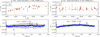 |
Fig. A.1 Resolving power Rλ = λ/Wλ of LAMOST MRS in the blue arm (left panels) and red arm (right panels) as measured in an example spectrum. In the upper panels, Rλ, for each setup, is plotted against wavelength for three fibers near the top, center, and bottom of the frame. The lower panels display the wavelength-averaged value of Rλ as a function of the fiber number. The mean R and its uncertainty is also reported in each of the lower panels. |
Appendix B Additional tables and figures
In this Appendix we provide supplementary figures and tables referenced in the main text to enhance the readability of the manuscript.
Radial velocities of the four new SB2 systems.
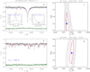 |
Fig. B.1 Example of the application of the code ROTFIT to the continuum-normalized spectrum (black dots) of J043925.00+184431.7 (= Gaia DR3 3409724027479793664). The red-arm and blue-arm spectrum is displayed in the upper left (a) and lower left (b) panels, respectively. In each panel the ELODIE template spectrum broadened at the v sin i of the target is overlaid with a full red line, while the best BT-Settl template is reproduced by a blue line. The difference between observed and template spectrum is shown by a dark-green line shifted upwards by 0.1 for the sake of clarity. The insets in panel a show the cross-correlation function (CCF) and the χ2 vs. v sin i. The right panels (c and d) display the χ2 maps in the Teff-log g plane for the red-arm and blue-arm spectrum, respectively. The 1σ contour is displayed by a red line, while the best-fitting parameters are marked with a blue dot in each panel. |
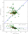 |
Fig. B.2 Comparison between the average radial velocities measured in this paper with those reported in the Gaia DR3 catalog. The orange dots denote stars with genuine radial velocity variations labeled as RVvar in Table 1. The one-to-one relation is shown by the solid blue line. The differences |

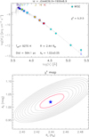 |
Fig. B.3 Top: Example of an SED fitting for the hot star J044636.9+190649 (= HD 285997). Bottom: χ2-contour map of the fitting. The red contour corresponds to the 1σ confidence level, while the best-fitting parameters (extinction and radius) are marked with a blue star symbol. |
Results of the SED fitting (extract).
Rotation periods derived in the present work (extract).
Notes. The full table is available at the CDS.
Rotation periods derived in the present work and in the literature.
 |
Fig. B.4 Top: Example of an SED fitting for the mid-F-type star J044831.8+185133 (= UCAC4 545-011022). Bottom: χ2-contour map of the fitting. The red contour corresponds to the 1σ confidence level, while the best-fitting parameters (extinction and radius) are marked with a blue star symbol. |
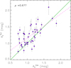 |
Fig. B.5 Comparison between the extinction values measured by us and by Zdanavičius et al. (2005). The one-to-one relation is displayed with a continuous green line, while the linear best fit to the data is shown with a magenta dashed line. |
 |
Fig. B.6 Gaia color–magnitude diagram of the cluster members (gray dots) showing the empirically defined lower envelope of the main sequence (red line). The color shift, ∆(GBP −GRP), for a star (indicated by a blue asterisk) is shown by the cyan horizontal segment, while the magnitude difference (∆G) relative to this envelope is marked with a purple vertical segment. The black arrow indicates the direction and length of the extinction vector for a reference value of AV = 1.1 mag. |
All Tables
Activity indicators: Net Hα equivalent width , line flux , and luminosity ratio (extract).
All Figures
|
Fig. 1 Left panel: spatial distribution of the NGC 1647 members according to Hunt & Reffert (2024, magenta dots), Cantat-Gaudin et al. (2018, blue dots), and Qin et al. (2026, green dots). The symbol size scales with the G magnitude. The red circles highlight the data points that correspond to objects observed with LAMOST MRS. The black squares enclose the three stars with UVES archive observations. The meaning of the symbols is also indicated in the legend. Middle panel: color–magnitude diagram of the same sources. The arrow indicates the extinction vector for a value of AV = 1.1 mag. Right panel: proper motion diagram of all the Gaia DR3 sources with G ≤ 16 mag (small gray dots) in the field of NGC 1647 (center coordinates RA(2000) = 71.5◦, Dec(2000) = +19◦, radius=3◦). The cluster members are highlighted with the same symbols as in the other panels (red circles have been omitted to avoid confusion). The violet asterisk denotes the average proper motion of the cluster according to Hunt & Reffert (2024) and the violet ellipse is the 5σ contour. |
| In the text | |
|
Fig. 2 Comparison between the radial velocities measured from blue-and red-arm LAMOST MRS spectra (top panel). Blue and red symbols are used for the hot and cool stars, analyzed with BT-Settl and ELODIE grids of templates, respectively. The symbol size scales with the v sin i of the source. The one-to-one relation is shown by the solid green line. The differences |
| In the text | |
|
Fig. 3 Comparison of the atmospheric parameters derived from the blue- and red-arm LAMOST MRS spectra using ROTFIT. The panels, from left to right, show the effective temperature (Teff), surface gravity (log g), metallicity ([Fe/H]), and projected rotation velocity (v sin i). The symbols are consistent with those presented in Fig. 2. We note the significantly larger rms dispersion observed for the Teff of the hot stars (blue data points). |
| In the text | |
|
Fig. 4 Radial velocity distribution obtained from all analyzed LAMOST MRS spectra of the cluster members (green histogram). Separate distributions are shown for the slowly rotating and fast rotating stars, as indicated in the legend. The best-fit Gaussian function applied specifically to the slowly rotating stars histogram is overplotted as a solid cyan line; its center (µ) and dispersion (σ) are also marked. The cluster Vr measured by Carrera et al. (2022) is indicated by the vertical yellow bar. The downward blue arrows highlight lower-probability targets (those not included in the golden sample) that lie outside the 5σ limit of the Gaussian center. Within this same velocity range, the orange dots denote the mean Vr of sources exhibiting variable radial velocity. |
| In the text | |
|
Fig. 5 Metallicity ([Fe/H]) distribution for all the cool stars of NGC 1647 (green histogram) and for the high-probability golden sample (purple histogram). The best-fit Gaussian function is overlaid as a solid black line; its center (µ) and dispersion (σ) are also marked. The cyan line denotes the weighted average of our [Fe/H] measures. The weighted-average metallicity measured by Carrera et al. (2022) for the two giants of the cluster is indicated by the vertical yellow bar, with the associated uncertainty represented by the hatched histogram. |
| In the text | |
|
Fig. 6 Extinction distribution for all the NGC 1647 members with LAMOST data (green histogram) and for the stars analyzed by Zdanavičius et al. (2005) (Zda05, orange histogram). The average AV values from the two datasets are marked with vertical solid lines and are reported in the corresponding color in the upper left corner of the panel. |
| In the text | |
|
Fig. 7 Spatial distribution of the stars in our sample. The symbols are color-coded according to their individual AV values. The grayscale image in the background is the 100 µm IRAS flux map. |
| In the text | |
|
Fig. 8 HR diagram for NGC 1647. The MS stars are denoted with dots (red for LAMOST MRS and cyan for UVES spectra). The orange squares represent the two giants studied by Carrera et al. (2022). PARSEC isochrones (Nguyen et al. 2022) at 100, 150, 200, and 300 Myr for models with the cluster metallicity ([Fe/H] = −0.08 dex) are overlaid. Green squares enclose the lower-probability members indicated by arrows in Fig. 4. |
| In the text | |
|
Fig. 9 Hα luminosity ratio |
| In the text | |
|
Fig. 10 Fit to the lithium depletion pattern of the EWLi measured in this work obtained with the EAGLES code (Jeffries et al. 2023). |
| In the text | |
|
Fig. 11 Rotation periods vs. the dereddened color index (GBP − GRP)0 for the members of NGC 1647 (black crosses). The periods of Pleiades (τ ≃ 125 Myr) members based on K2 (Rebull et al. 2016) and TESS (Frasca et al. 2025) are overplotted as orange dots, while those of NGC 3532 (τ ≃ 300 Myr) members (Fritzewski et al. 2021) are shown as blue dots for comparison. |
| In the text | |
|
Fig. 12 Projected rotational velocity (v sin i) vs. the Gaia color shift ∆(GBP −GRP). The color shift is measured relative to the lower envelope of the MS strip (Fig. B.6). The Pearson’s correlation coefficients (ρ) is marked in the upper right corner of the panel. |
| In the text | |
|
Fig. 13 Extinction (AV) vs. the Gaia color shift ∆(GBP − GRP). The data derived in the present work and by Zdanavičius et al. (2005) are distinguished by different colors, as indicated in the legend. The linear best fits to our data and to the Zdanavičius et al. (2005) data are shown as a green dashed line and an orange dot-dashed line, respectively. The Pearson’s correlation coefficients (ρ) are also marked in the upper left corner. |
| In the text | |
|
Fig. A.1 Resolving power Rλ = λ/Wλ of LAMOST MRS in the blue arm (left panels) and red arm (right panels) as measured in an example spectrum. In the upper panels, Rλ, for each setup, is plotted against wavelength for three fibers near the top, center, and bottom of the frame. The lower panels display the wavelength-averaged value of Rλ as a function of the fiber number. The mean R and its uncertainty is also reported in each of the lower panels. |
| In the text | |
|
Fig. B.1 Example of the application of the code ROTFIT to the continuum-normalized spectrum (black dots) of J043925.00+184431.7 (= Gaia DR3 3409724027479793664). The red-arm and blue-arm spectrum is displayed in the upper left (a) and lower left (b) panels, respectively. In each panel the ELODIE template spectrum broadened at the v sin i of the target is overlaid with a full red line, while the best BT-Settl template is reproduced by a blue line. The difference between observed and template spectrum is shown by a dark-green line shifted upwards by 0.1 for the sake of clarity. The insets in panel a show the cross-correlation function (CCF) and the χ2 vs. v sin i. The right panels (c and d) display the χ2 maps in the Teff-log g plane for the red-arm and blue-arm spectrum, respectively. The 1σ contour is displayed by a red line, while the best-fitting parameters are marked with a blue dot in each panel. |
| In the text | |
|
Fig. B.2 Comparison between the average radial velocities measured in this paper with those reported in the Gaia DR3 catalog. The orange dots denote stars with genuine radial velocity variations labeled as RVvar in Table 1. The one-to-one relation is shown by the solid blue line. The differences |
| In the text | |
|
Fig. B.3 Top: Example of an SED fitting for the hot star J044636.9+190649 (= HD 285997). Bottom: χ2-contour map of the fitting. The red contour corresponds to the 1σ confidence level, while the best-fitting parameters (extinction and radius) are marked with a blue star symbol. |
| In the text | |
|
Fig. B.4 Top: Example of an SED fitting for the mid-F-type star J044831.8+185133 (= UCAC4 545-011022). Bottom: χ2-contour map of the fitting. The red contour corresponds to the 1σ confidence level, while the best-fitting parameters (extinction and radius) are marked with a blue star symbol. |
| In the text | |
|
Fig. B.5 Comparison between the extinction values measured by us and by Zdanavičius et al. (2005). The one-to-one relation is displayed with a continuous green line, while the linear best fit to the data is shown with a magenta dashed line. |
| In the text | |
|
Fig. B.6 Gaia color–magnitude diagram of the cluster members (gray dots) showing the empirically defined lower envelope of the main sequence (red line). The color shift, ∆(GBP −GRP), for a star (indicated by a blue asterisk) is shown by the cyan horizontal segment, while the magnitude difference (∆G) relative to this envelope is marked with a purple vertical segment. The black arrow indicates the direction and length of the extinction vector for a reference value of AV = 1.1 mag. |
| In the text | |
Current usage metrics show cumulative count of Article Views (full-text article views including HTML views, PDF and ePub downloads, according to the available data) and Abstracts Views on Vision4Press platform.
Data correspond to usage on the plateform after 2015. The current usage metrics is available 48-96 hours after online publication and is updated daily on week days.
Initial download of the metrics may take a while.