


| Issue |
A&A
Volume 710, June 2026
|
|
|---|---|---|
| Article Number | A201 | |
| Number of page(s) | 24 | |
| Section | Extragalactic astronomy | |
| DOI | https://doi.org/10.1051/0004-6361/202659090 | |
| Published online | 26 June 2026 | |
The January 2010 flare of Mrk 421: Insights from a stochastic acceleration model
1
Japanese MAGIC Group: Department of Physics, Tokai University, Hiratsuka 259-1292, Kanagawa, Japan
2
Japanese MAGIC Group: Department of Physics, Kyoto University, 606-8502 Kyoto, Japan
3
ETH Zürich, CH-8093 Zürich, Switzerland
4
Università di Siena and INFN Pisa, I-53100 Siena, Italy
5
Institut de Física d’Altes Energies (IFAE), The Barcelona Institute of Science and Technology (BIST), E-08193 Bellaterra (Barcelona), Spain
6
Universitat de Barcelona, ICCUB, IEEC-UB, E-08028 Barcelona, Spain
7
Instituto de Astrofísica de Andalucía-CSIC, Glorieta de la Astronomía s/n, 18008 Granada, Spain
8
Università di Padova and INFN, I-35131 Padova, Italy
9
National Institute for Astrophysics (INAF), I-00136 Rome, Italy
10
Max-Planck-Institut für Physik, D-85748 Garching, Germany
11
Instituto de Astrofísica de Canarias and Dpto. de Astrofísica, Universidad de La Laguna, E-38200 La Laguna, Tenerife, Spain
12
Croatian MAGIC Group: University of Zagreb, Faculty of Electrical Engineering and Computing (FER), 10000 Zagreb, Croatia
13
Saha Institute of Nuclear Physics, A CI of Homi Bhabha National Institute, Kolkata 700064, West Bengal, India
14
Centro Brasileiro de Pesquisas Físicas (CBPF), 22290-180 URCA, Rio de Janeiro (RJ), Brazil
15
IPARCOS Institute and EMFTEL Department, Universidad Complutense de Madrid, E-28040 Madrid, Spain
16
Japanese MAGIC Group: Institute for Cosmic Ray Research (ICRR), The University of Tokyo, Kashiwa, 277-8582 Chiba, Japan
17
University of Lodz, Faculty of Physics and Applied Informatics, Department of Astrophysics, 90-236 Lodz, Poland
18
Centro de Investigaciones Energéticas, Medioambientales y Tecnológicas, E-28040 Madrid, Spain
19
Departament de Física, and CERES-IEEC, Universitat Autònoma de Barcelona, E-08193 Bellaterra, Spain
20
Università di Pisa and INFN Pisa, I-56126 Pisa, Italy
21
INFN MAGIC Group: INFN Sezione di Bari and Dipartimento Interateneo di Fisica dell’Università e del Politecnico di Bari, I-70125 Bari, Italy
22
Department for Physics and Technology, University of Bergen, Bergen, Norway
23
Università di Udine and INFN Trieste, I-33100 Udine, Italy
24
INFN MAGIC Group: INFN Sezione di Torino and Università degli Studi di Torino, I-10125 Torino, Italy
25
Croatian MAGIC Group: University of Rijeka, Faculty of Physics, 51000 Rijeka, Croatia
26
Universität Würzburg, D-97074 Würzburg, Germany
27
Technische Universität Dortmund, D-44221 Dortmund, Germany
28
Japanese MAGIC Group: Physics Program, Graduate School of Advanced Science and Engineering, Hiroshima University, 739-8526 Hiroshima, Japan
29
Armenian MAGIC Group: ICRANet-Armenia, 0019 Yerevan, Armenia
30
Croatian MAGIC Group: Josip Juraj Strossmayer University of Osijek, Department of Physics, 31000 Osijek, Croatia
31
Finnish MAGIC Group: Finnish Centre for Astronomy with ESO, Department of Physics and Astronomy, University of Turku, FI-20014 Turku, Finland
32
University of Geneva, Chemin d’Ecogia 16, CH-1290 Versoix, Switzerland
33
Inst. for Nucl. Research and Nucl. Energy, Bulgarian Academy of Sciences, BG-1784 Sofia, Bulgaria
34
INFN MAGIC Group: INFN Sezione di Catania and Dipartimento di Fisica e Astronomia, University of Catania, I-95123 Catania, Italy
35
Finnish MAGIC Group: Space Physics and Astronomy Research Unit, University of Oulu, FI-90014 Oulu, Finland
36
Japanese MAGIC Group: Institute for Space-Earth Environmental Research and Kobayashi-Maskawa Institute for the Origin of Particles and the Universe, Nagoya University, 464-6801 Nagoya, Japan
37
INFN MAGIC Group: INFN Roma Tor Vergata, I-00133 Roma, Italy
38
Como Lake centre for AstroPhysics (CLAP), DiSAT, Università dell’Insubria, via Valleggio 11, 22100 Como, Italy
39
Port d’Informació Científica (PIC), E-08193 Bellaterra (Barcelona), Spain
40
Department of Physics, University of Oslo, Oslo, Norway
41
Dipartimento di Fisica, Università di Trieste, I-34127 Trieste, Italy
42
Dipartimento di Fisica, Università di Roma Tor Vergata, Via della Ricerca Scientifica, 1 Roma I-00133, Italy
43
INAF - Osservatorio Astronomico di Padova, Padova, Italy
44
Japanese MAGIC Group: Institute for Cosmic Ray Research (ICRR), The University of Tokyo, Kashiwa, 277-8582 Chiba, Japan
45
Space Science Data Center, Agenzia Spaziale Italiana, Via del Politecnico snc, 00133 Roma, Italy
46
INAF Osservatorio Astronomico di Roma, Via Frascati 33, 00078 Monte Porzio Catone (RM), Italy
★ Corresponding authors: This email address is being protected from spambots. You need JavaScript enabled to view it.
Received:
22
January
2026
Accepted:
22
April
2026
Abstract
Context. Mrk 421 displayed its highest flux state ever observed in February 2010 with very high tera-electronvolt fluxes and interesting cross-band correlations and a spectral energy distribution (SED) evolution not entirely consistent with the standard single zone leptonic synchrotron self-Compton model. The source was already in a high state in January 2010 and displayed strong variability in the days preceding the highest state. We study the temporal evolution of the spectra in January to extract information about the particle dynamics and the physical properties of the emission region.
Aims. We build on the temporal variability and correlations studied in our previous work and attempt to improve the SED model fits with a physics-oriented approach.
Methods. The The multi-wavelength data were processed and the SEDs were fit using JetSeT. The SED evolution and cross-band correlations were modelled using leptonic log-parabola with a low energy power-law branch (LPPL) and pile-up distributions that are predicted in a stochastic acceleration scenario. A simplified temporal evolution model was developed and fitted to the SEDs and the resulting trends and phenomenology were characterised in the context of the theoretical literature. An expanding emission region model was also tested.
Results. We find the spectral variability to be in good agreement with stochastic acceleration. Our analysis suggests that the standard LPPL distribution develops a Maxwellian pile-up component at the transition from the acceleration-dominated to the cooling-dominated phase on 3 nights in the dataset, as is also hinted at by the very-high energy and X-ray light curves. The resulting phenomenology of our sequential snapshot evolution SED model agrees well with theoretical and numerical simulation studies on temporal evolution using the diffusion equation approach. Curvature in the electron energy distribution (EED) anti-correlates with the synchrotron peak frequency, as was expected from stochastic acceleration. We tested an alternate model with expanding emission region and the resulting EED spectral index, expansion velocity, and magnetic field index agree with prior works using datasets collected in different flaring states of the source.
Key words: acceleration of particles / galaxies: active / BL Lacertae objects: individual: Mrk421
© The Authors 2026
 Open Access article, published by EDP Sciences, under the terms of the Creative Commons Attribution License (https://creativecommons.org/licenses/by/4.0), which permits unrestricted use, distribution, and reproduction in any medium, provided the original work is properly cited.
This article is published in open access under the Subscribe to Open model. This email address is being protected from spambots. You need JavaScript enabled to view it. to support open access publication.
1. Introduction
Blazars, a class of jetted active galactic nuclei (AGN), are known to be highly variable in the X-ray and very-highenergy(VHE) γ-ray (E > 100 GeV) bands. The blazar jet is powered by the supermassive black hole in the central regions of these AGN and emission is beamed towards the observer, enhancing the intrinsic variability by relativistic effects. The archetypal blazar Markarian 421 (Mrk421) (z = 0.031; de Vaucouleurs et al. 1991) belongs to the high synchrotron peaked (HSP) BL Lac object category as per the unified blazar sequence (Urry & Padovani 1995; Fossati et al. 1998) with the synchrotron peak around 1017 Hz, although the validity of this classification scheme has been called into question by more recent large-sample-size studies (Keenan et al. 2021; Prandini & Ghisellini 2022). The VHE flux of Mrk 421 often changes by an order of magnitude between the flaring and quiet states.
Mrk 421 has been known to show a variety of spectral characteristics during different flaring periods (Baloković et al. 2016; MAGIC Collaboration 2021; Acciari et al. 2020; Dmytriiev et al. 2021). The general structure of its spectral energy distribution (SED) agrees well with a single-zone self-Compton (SSC) model (e.g. Aleksić et al. 2015b) typically used for modelling BL Lac objects objects owing to the lack of evidence of external photon fields (see Böttcher (2019) for an overview of blazar modelling). However, these single and even multi-zone models are a highly simplified description of the emission from a complex object spanning several kiloparsecs. Mrk 421 in particular is well known for showing strong variations in the X-ray and VHE γ-ray flux over short timescales (Arbet-Engels et al. 2021; Gokus et al. 2024; Abe et al. 2026), which makes it important to consider this temporal variability aspect in any spectral modelling attempts.
The ‘snapshot’ approach has often been used in the past to study the time-averaged emission of blazar jets. To build such a snapshot, quasi-simultaneous multi-wavelength (MWL) observations are combined depending on the brightness of the source in different bands, which are then usually modelled independent of each other. The dynamics of the particle population are abstracted out using parametrised steady-state solutions to the diffusion equation. This approach leads to the loss of some physics information contained in the evolution of the states. In contrast, temporal evolution models can provide more information about the relativistic flows and emission environments in the jet. These models use a self-consistent diffusion equation approach to model the time evolution of the particle population that drives the photon emission.
The dramatic activity of Mrk 421 in 2010 was covered in an extensive MWL campaign (Aleksić et al. 2015b; Abeysekara et al. 2020) from the radio to VHE bands. While the highest flux in the X-ray and VHE bands was seen in February 2010 (see models in Aleksić et al. 2015b; Dmytriiev et al. 2021), the cadence of spectral data in this period is sparse compared to January 2010, when it is possible to build daily timescale snapshots. This rich dataset from January allows us to extract the physical information regarding the acceleration of particles and the emission environment in the jet. The daily binned SEDs (in the observer reference frame) minimise contamination due to averaging of different spectral states. Additionally, we treated the SED dataset as a sequence of states instead of as completely independent states, bringing our method closer to a temporal evolution model compared to the typical snapshot model. We combined this approach with a physically motivated particle distribution under the stochastic acceleration framework. This allowed us to probe the jet state transitioning between acceleration and cooling domination. The results of this study will be used to guide a fully self-consistent temporal evolution model in a future work.
In Sect. 2 we describe the processing and data reduction into a series of SEDs, while the fitting procedure and the physical set-up of the models is explained in Sect. 3. The results are reported in Sect. 4 with the associated phenomenology and physics interpretation in Sect. 5. We build an expanding emission region model based on these results in Sect. 6 and provide conclusions, caveats, and our outlook for the future in Sect. 7. Additional information on data processing and some plots for individual models that are not directly relevant to the discussion can be found in the appendix.
2. Observations and data reduction
This section describes the instrument-specific processing relevant to building the SEDs sequence and the observations that motivate the physics-oriented approach to setting up the emission region in Sect. 3. The full MWL light curve (LC) dataset can be found in Abe et al. (2025), while a summary of the analysis done for the individual instruments can be found in Appendix B.
Figure 1 shows the VHE and X-ray LCs, which were the bands with the strongest variability and historic high flux levels during the 2009–2010 observation campaign, while Fig. 2 shows the January 2010 dataset. The well-sampled MWL LC and the multiple flaring incidents with the flux changing by a factor of ∼3 in a matter of days motivated us to study January 2010 in detail. The January dataset was used to build and label the SEDs by Major Atmospheric Gamma Imaging Cherenkov (MAGIC) telescope observation start date as described in Sect. 2.1.
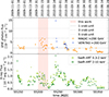 |
Fig. 1. VHE and X-ray LC of Mrk 421 during the 2009–2010 MAGIC observation campaign. The data were daily binned and taken from Abe et al. (2025). Our broadband SED modelling was performed over the period highlighted with a vertical red band (January 2010). Figure 2 shows the MWL data in the highlighted region in more detail. |
2.1. γ-ray bands
We binned the spectral data according to the availability of the MAGIC telescope observations. There are 16 nights in our SED dataset, starting from 08 January 2010 until 26 January 2010, and the MWL SEDs are labelled according to the date on which MAGIC observations started. Given the duty cycle and observation schedules of ground-based Imaging Atmospheric Cherenkov Telescopes (IACTs), it is hard to obtain evenly sampled datasets, so the MWL observations were assigned to the temporally closest MAGIC observation. This assumes that a few short observations within a few hours of each other are contemporary and representative of the general behaviour of the source over multi-hour timescales. Abe et al. (2025) found significant intra-night variability on 15 January 2010 with flux changing by a factor of ∼2 on sub-hour timescales at a 3.7σ level. However the rest of the dataset during January 2010 showed no such intra-night variability, which supports the idea of the source being stable during individual VHE observations.
Given the sensitivity of Fermi-Large Area Telescope (Fermi-LAT) and the flux of Mrk 421 in the high energy (HE) (∼106 − 10 eV) band, it was not possible to obtain statistically significant energy bins for a large fraction of the dataset at daily timescales (see Appendix B for details) for the Fermi-LAT observations. Thus, a 3-day binning was used with the closest 3-day bin matched with each MAGIC observation night. Even with the 3-day bins, there are some nights in the dataset with a very large uncertainty in the spectrum. However, the variability in the HE band is low as quantified by the fractional variability in Abe et al. (2025) and we do not expect interesting dynamics in the HE band on the daily timescales for this particular source and the 2010 flare. To account for inter-instrument calibration effects, we added 20% systematic uncertainty to the MAGIC data and 10% to the Fermi-LAT data (see Table 1) based on the published instrument performance (Abdo et al. 2009; Aleksić et al. 2016).
2.2. X-ray bands
We converted the hard X-ray (> 10 keV) excess count observed by Swift Burst Alert Telescope (Swift-BAT) to crab units and subsequently to a spectral point using the method described in Krimm et al. (2013). As was described by the authors, the systematic uncertainties in the spectral points thus obtained are large and we added a 30% uncertainty to this data (Table 1) during the modelling. Additionally, for days with negative excess counts due to background fluctuations, no spectral points can be extracted (14 and 26 January). Despite this, the Swift-BAT data turned highly useful on 19 January when the peak of the synchrotron bump of the SED was outside the energy range of the Swift X-ray Telescope (Swift-XRT), and hence it would be hard to constrain the peak position without the Swift-BAT spectral point.
The data from the Swift-XRT were processed as described in Abe et al. (2025). The X-ray band spectral points at the edges of the ranges in the 0.3 − 2 keV and 2 − 10 keV bands of the Swift-XRT were additionally checked for energy dependence of systematic uncertainties, since the observed curvature in the data points directly affects the conclusions of our SED modelling. Uncertainty in the neutral Hydrogen (nH) density along the line of sight to Mrk 421 can mimic additional curvature (see Appendix B.3). This systematic uncertainty was included in the SED modelling and the conclusions regarding the curvature were unaffected.
2.3. UV-optical and radio data
We used the combined dataset from Abe et al. (2025) to generate our SEDs for Swift UV-Optical Telescope (Swift-UVOT), R-band, and radio bands. We combined the data to build as contemporaneous a SED as possible, using the MWL data that was temporally closest to the VHE observation. We used a 10% systematic uncertainty in the ultraviolet (UV) and optical band data, which is above the typical uncertainty assumed in these bands (Baloković et al. 2016; Acharyya et al. 2023).
The radio band emission is expected to originate from larger regions in the jet due to the synchrotronself-absorption (SSA) process (see for e.g. Tramacere et al. 2022) compared to the compact regions close to the central supermassive black hole (SMBH) emitting higher-energy photons. Hence, we restricted the minimiser to the spectral points with ≥1011 Hz to exclude the lowest-energy radio data that are strongly affected by SSA. Typical systematic flux uncertainty for the individual telescopes and radio bands for our dataset range from 2 − 10% (Richards et al. 2011; Partridge et al. 2016) but we used a 20% value in our modelling to account for the multiple different telescopes and the uneven sampling. A more detailed description of the data processing can be found in Appendix B.
2.4. Data phenomenology
The X-ray LC has peaks around 15 and 19 January, and the VHE LC follows a similar trend with peaks on 14 and 20 January. These peaks hint at multiple re-acceleration and/or injection episodes. Combined with the variability and curvature information described in the subsequent paragraphs, this could be seen as a sign of a change from acceleration-dominated to cooling-dominated evolution, plausibly from weakening injection or reduced acceleration efficiency of the particle population driving the emission. We exploit this information in Sect. 3.1 to motivate a particle distribution function to capture the physics of this transition. This also differentiates the January flare from the February and March flares, which show a single peak followed by a consistently decreasing flux (Aleksić et al. 2016) indicative of a cooling-dominated phase that is especially noticeable in the denser sampling of the X-ray band in Fig. 1.
Abe et al. (2025) carried out a detailed study of temporal variability and MWL cross-correlation and we report the results that are relevant to our analysis here. The dataset shows the typical two-peak structure in the fractional variability (Fvar; Vaughan et al. 2003), with the X-ray and VHE bands showing the highest Fvar > 0.8. Moreover, there was no delay between the X-ray and VHE bands in the full 7-month-long period, suggesting a co-spatial origin of the emission. Significant correlation and similar values of fractional variability were seen between the UV and HE γ-ray bands, making the overall MWL picture consistent with the standard SSC scenario used to model the broadband emission of Mrk 421. There was no correlation between the UV and X-ray data and a weak correlation between UV and the VHE band, which was interpreted by the authors as a multi-zone scenario with a compact VHE emission zone embedded in a larger zone emitting at lower energies. However, given the longer synchrotron cooling times of electrons emitting at UV energies versus the ones emitting at X-rays, the correlation between these bands can be weak even in a single-zone scenario. We use a single-zone SSC scenario in this work to minimise the degeneracies in the model as the parameter space is not fully constrained, with the goal of studying the acceleration-cooling domination transition hinted at by the LC using a physically motivated electron energy distribution (EED).
Since the shape of the underlying EED and stochastic acceleration can affect the curvature in the synchrotron peak (Massaro et al. 2004, 2006; Tramacere et al. 2007), we tested for a log-parabolic curvature at the peak of the synchrotron bump. The peak of the synchrotron emission lies in the Swift-XRT energy window for Mrk 421, the XSPEC analysis of the Swift-XRT data found that the log-parabola was a better fit than a power law with a very high significance (≫5σ) for all days in January 2010. This analysis, however, gave a distorted picture of the phenomenology, as is seen later in Sect. 4, since on 19 January the peak position clearly lies outside the Swift-XRT energy and the log-parabolic fit reports a very small curvature, contrary to the true picture with a very large curvature shown by the MWL dataset. Thus, we performed a log-parabolic fit to a larger frequency range, from UV to X-ray bands (Swift-UVOT, Swift-XRT, and Swift-BAT data). The results of the analysis can be seen in Fig. 3, with an anti-correlation trend between the peak frequency ( ) and the log-parabolic curvature measured in the UV–X-ray range (bsync). This behaviour is expected in a stochastic acceleration scenario, which was then used to choose the parametrised form of the EED as described in Sect. 3.1.
3. SED modelling
The SED modelling was carried out using JetSeT1 v1.3.1 (Tramacere 2020). The input relativistic particle distribution radiates via synchrotron and inverse Compton (IC) processes, and all relevant internal absorption processes are also included in the code (SSA and γ-γ photo-absorption). The software is capable of evolving the particle distribution in a self-consistent time-dependent approach considering acceleration and radiative cooling. The parameter space of such fully self-consistent time-dependent models is much larger than that of snapshot models. This highly complicates the implementation of a single time-evolving model to account for all the complex time variability and phenomenology shown by Mrk 421. Hence, we start with a snapshot model using phenomenological EEDs sensitive to cooling and acceleration, driven by hints of stochastic acceleration seen in Figs. 2 and 3. The current analysis will build the baseline for future temporal evolution studies of this flare.
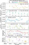 |
Fig. 2. MWL LC during January 2010 from radio to VHE. The data were taken from Abe et al. (2025). The top axis is marked with a date colour key, which is consistent across the plots and tables in the paper. |
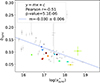 |
Fig. 3. Anti-correlation between the peak curvature (bsync) vs the log10 of the peak frequency ( |

3.1. Particle population distribution
The observations provide a rich phenomenology, with the source going through a complex pattern of acceleration and cooling-dominated episodes. The acceleration and cooling timescales are a function of electron energy and the physics of the acceleration and cooling processes. In all subsequent mentions, we refer to these timescales for electrons emitting in the X-ray and VHE bands, where the largest spectral variability occurs. Modelling this phenomenology is a challenging task, since the competition between cooling and acceleration timescales adds further degeneracies to the ones intrinsic to the SSC scenario, plus the possible coexistence of multiple emitting regions. Hence, we focus on a one-zone SSC leptonic scenario, based on an EED with parameters sensitive to both the cooling and the acceleration processes during flaring sequences.
The physics of these processes can be captured self-consistently using differential kinetic equations (see Ramaty 1979; Becker et al. 2006; Tramacere et al. 2011). In particular, as a consequence of stochastic Fermi acceleration in a turbulent magnetic field, analytical and numerical solutions of the kinetic equations naturally lead to the formation of a log-parabola with a low energy power-law branch (LPPL) EED (Stawarz & Petrosian 2008; Tramacere et al. 2009, 2011) through the momentum-diffusion process. The LPPL EED consists of a power-law low energy branch characterised by a spectral index, s, and a log-parabolic high energy branch with curvature, r. This provides a good description of the EED, as long as the process is in the acceleration-dominated regime; that is, the electron acceleration times are shorter than the cooling times. The low-energy branch power-law index, s, can be driven by either the first-order or the second-order Fermi processes, depending on the efficiency of confinement of the particles within the acceleration region. The log-parabolic curvature, r, is driven by the momentum-diffusion process, and its value can be used to track the evolution of the system from an acceleration- to cooling-dominated regime (Tramacere et al. 2011). In this regard, and based on the spectral patterns described in 2.4, specifically the log-parabolic shape observed in the X-ray window, we modelled the January 2010 period with a LPPL distribution. Mono-energetic relativistic particles are assumed to be injected into the acceleration region at Lorentz factor γ = γinj, which can be of the order of ∼102 − 103 as a consequence of electron preheating within (mildly relativistic) electron-ion plasma shocks (Zech & Lemoine 2021; Arbet-Engels et al. 2025). An additional simple power-law component develops for γ ≤ γinj in the EED at equilibrium because of the cooling of particles at higher energies (Rybicki & Lightman 1986). The acceleration process is also limited at the highest energies by an exponential cut-off. The overall particle number density distribution can be parametrised in the following way (Tramacere et al. 2011):
 (1)
(1)
 (2)
(2)
 (3)
(3)
where γ0 is the onset of the spectral curvature r, γc is the limit of the acceleration process, and a is the cut-off index. For our LPPL model, γc = 1 × 10⁷, capping the maximum energies the particles can be accelerated to, and a = 1, which yields the standard exponential cut-off functional form. This choice of γc is consistent with the lack of an observation of an exponential cut-off in the X-ray data and avoids a non-physical sharp cut-off at the high-energy edge of the numerical grid of γ. Hence, we have a total of four free parameters for the LPPL distribution used in the modelling (γinj, γ0, s, r).
We found that this EED parametrisation provides a good description for most of the SEDs in our dataset, but failed to capture the curvature seen in the synchrotron peak of the SED on some days, especially 19 January 2010. This suggested that some of these states, which were all close to the peak of the flares, could be the result of the transition of the system towards a cooling-dominated regime.
When the system moves from an acceleration-dominated to a cooling-dominated regime, i.e. when the acceleration timescales become longer than the cooling timescales, a fraction of the population can ‘thermalise’ close to the equilibrium energy where the acceleration and cooling effects are balanced. As a result, the formation of a pile-up component (Schlickeiser 1984, 1985; Stawarz & Petrosian 2008) described by a relativistic Maxwellian distribution is expected at the high-energy tail of the EED. Such a transition might be triggered by changes in the acceleration efficiency, variations in the injection luminosity of the leptons, or sudden changes in the jet environment; however, the approach in this work cannot distinguish between these scenarios and we defer testing these cases to a future work. Instead, we used a parametric distribution to capture the signature of this transition in the spectra. The radiative signature of such a pile-up appears close to the SED peak frequencies, i.e. in the X-ray and VHE bands in the case of HSP blazars. The general form of the Maxwellian component is as follows (Stawarz & Petrosian 2008):
 (4)
(4)
which can be combined with a power law to get the final EED with pile-up
 (5)
(5)
 (6)
(6)
where the same cut-off function as the LPPL case applies (Eq. (2)). Here, γc is the acceleration-cooling equilibrium Lorentz factor and a depends on the dominant cooling process and the magnetic turbulence index (parameter q in Stawarz & Petrosian 2008). f is a scale factor for the relative strength of the pile-up with respect to the standard power-law component. This functional form is an analytical simplification of the equilibrium approximations of simulated mono-energetic particle injection and evolution under stochastic acceleration and radiative cooling using the diffusion equation approach, as seen in Stawarz & Petrosian (2008) and Tramacere et al. (2011).
The pile-up EED defined above has a total of five free parameters (γinj, γc, s, a, f). We fitted the LPPL and pile-up EED to all the SED and compared the fits via a likelihood ratio test described in Sect. 4. For plots visualising the EED in the subsequent text, we use the γ2n(γ) distribution instead of just n(γ) to emphasise and compare the curvature in the EED. However, for simplicity, we shall keep referring to the γ2n(γ) distribution as the EED.
3.2. Physical set-up of the emitting zone
The emission region is assumed to be a spherical blob with radius R that is permeated by a tangled magnetic field of strength B. The particle density in the emitting region is given by N. The emitting plasma moves relativistically towards the observer with a bulk Lorentz factor, Γ. This leads to relativistic beaming of the radiation with a Doppler factor, δ, of ∼Γ. Finally, the ratio of relativistic electrons to cold protons, which influences the jet power computation, is fixed to 1 in our modelling.
3.3. Model fitting procedure: ‘Parallel’ and ‘sequential’ fits
We fitted our model to the daily binned SEDs of the January 2010 epoch. In particular, we focused on the evolution of the EED whose shape is physically motivated assuming stochastic acceleration (see Sect. 3.1) to obtain insights into the cooling and acceleration processes at play.
We performed an initial fit of each SED independently using a frequentist approach via iMinuit to minimise the χ2. Since the parameters for each day were independent of each other, we refer to this as the ‘parallel fit’. The parallel fitting process was repeated a few times iteratively, which allowed us to restrict the fit ranges and to identify parameters that can be reasonably kept constant without significantly degrading the goodness of fit. The Doppler beaming factor, δ, was fixed to 45 in agreement with the average value derived from preliminary fits, which did not reveal significant temporal variations. For a small angle of the jet axis with the observer line of sight as is the case for blazars (< 5°), δ ∼ Γ, which makes our choice of Doppler factor consistent with the typical bulk Lorentz factor used in the literature (Aleksić et al. 2015b; MAGIC Collaboration 2021; Banerjee et al. 2019).
In order to better capture the temporal evolution of the emitting region, we developed the ‘sequential fit’ procedure using the parameter values and ranges of the parallel fit to set up the model as described:
-
The parameter fit ranges in the sequential fit were set based on the maximum and minimum range of the parallel fit, with additional padding of 50% to avoid convergence on the boundary.
-
The parallel fit of the first SED (8 January 2010) was used as the starting point for the sequential fit. Subsequent SEDs used the best fit values obtained for the preceding day as initial guess, leading to a temporally evolving snapshot model.
-
We computed the sequential fit with the LPPL SED (nLPPL, Eq. (3)) as the baseline or reference, and then similarly with pile-upEED (npile − up, Eq. (6)) for each day.
-
We passed the best-fit model for both EEDs to a Markov chain Monte Carlo (MCMC) sampler (emcee2 interface in JetSeT) to get the Bayesian error bars and SED model ranges.
The comparison between the sequential fit results of the LPPL and pile-up model can be found in Sects. 4 and 5. In the fitting process, we found that on average the emitting region size, R, had the tendency to expand along with an anti-correlation with B and N (Sect. 5.5). This expansion is expected if the region travels downstream a jet with conical (or parabolic) shape. Motivated by these findings, we performed an additional investigation attempting to capture the physics of this expansion. This model is discussed in Sect. 6.
4. Best-fit model and results
4.1. Comparing the LPPL and pile-up models
Using the χ2 of the models with the LPPL and pile-up EED, we obtained the likelihood, ℒ, as  and subsequently the TS of the pile-up model as TSpile − up = −2 ln(ℒLPPL/ℒpile − up). Based on our sequential fitting strategy and a TS > 4 cut (p-value < 0.05), we found that the pile-up model was significant on 15, 19, and 20 January 2010. A comparison of the TS of the models can be seen in Table 2 including the reduced χ2 and the pile-up scale parameter, f. A major difference appears in the synchrotron peak shape and position, sharply evident on 19 January in Fig. 4 despite both models having a good fit to the data as indicated by the reduced χ2 (see Fig. C.1 for the same comparison for 15 and 20 January). The TS of the pile-up model is positive except on 12 and 21 January, although not always statistically significant. Since npile − up in Eq. (6) has a power law with an exponential cut-off that has a similar effect as the curvature in nLPPL (albeit an energy-dependent curvature compared to the constant curvature in the LPPL case), it can mimic the general shape of the LPPL distribution and produce similar χ2. However, the LPPL and pile-up distributions appear at different stages of the temporal evolution of the EED and on 12 and 21 January, the evolution could be in a strictly acceleration-dominated phase better described by the LPPL distribution.
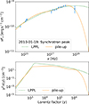 |
Fig. 4. Comparison of the synchrotron peak of the SED and the EED of the LPPL and pile-up models on 19 January. The top panel illustrates the optical-to-X-ray SED using the pile-up (orange line) and LPPL (dashed green line) EED on 19 January 2010, the day with the strongest indication of a pile-up (see Sect. 4). The bottom panel presents the corresponding EED, where n(γ) is the particle number density distribution. The full frequency range of this SED model can be seen in Fig. 6(i). |
Significance of the pile-up vs the LPPL EED model, with the days that have statistic (TS) > 4 (p-value < 0.05) highlighted in darker text. The TS is the likelihood ratio of the models.  is the reduced-χ2, where the numerator is the χ2 and the denominator is the number of degrees of freedom of the model. The 3 days that satisfy the TS threshold for pile-up are marked with a star marker, ‘✸’, on the phenomenology plots in Sects. 5 and 6, and Appendix D.
The best-fit parameter values are reported in Table 3. The temporal evolution of the parameters can be seen in Figs. 5 and C.4 for the LPPL and pile-up models, respectively.
 |
Fig. 5. LPPL model results. The marker with the error bar represents [0.15, 0.50, 0.85] quantiles of 104 MCMC realisations and the short horizontal dashes represent the [0.01, 0.99] quantile range. |
MCMC sampler results for the models LPPL and pile-up models.
4.2. Combining the LPPL and pile-up models
Based on the results reported in the previous sections, we combined the LPPL and pile-up models by picking the results from the pile-up model on 15, 19, and 20 January when TSpile − up > 4. This requires an additional step, however, since simply mixing the model results breaks the sequential fit approach. The resulting fits in each sequential fit step depend on the prior step’s best fit, which would not be the case if we just mixed the results. Thus, to properly combine the models, we ran our sequential fitting pipeline again with the EED changed from LPPL (nLPPL, Eq. (3)) to pile-up (npile − up, Eq. (6)) for the days when pile-up was significant, carrying over the compatible parameters (s and γinj). This model will be referred to as the ‘combined model’ henceforth.
4.3. SED fits for the combined model
The Bayesian 98% quantile model ranges of the SED fits of the combined model is shown in Fig. 6 from 14 January to 20 January. The remaining days are included in Fig. A.1. While the biggest difference in the LPPL and pile-up models was in the synchrotron peak (Fig. 4), pile-up can also appear as a narrow feature in the VHE spectrum as hinted by the residuals of 15 and 19 January in panels (f) and (i) of Fig. 6. Narrow features in the VHE spectrum have been reported by MAGIC Collaboration (2020) for Mrk 501 and were hinted at for Mrk 421 in Aleksić et al. (2015b) in March 2010; however, in our case this effect was small compared to the systematic uncertainty of the MAGIC telescopes, requiring further specialised analysis of the data. In our analysis, the hint of pile-up is mostly suggested by the X-ray spectra (Sect. 2.2). Although the synchrotron peak frequency of Mrk 501 lies completely outside the Swift-XRT energy range and the peak shape is not fully sampled by the data, a hint of pile-up was also present in the Swift-BAT spectral point in MAGIC Collaboration (2020).
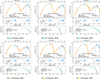 |
Fig. 6. SED fits: Combined model. The best fit and MCMC range for the SED (top subplot) and the EED (bottom subplot) for each observation date in January 2010 are shown. The residuals of the model and the χ2, reduced χ2 ( |

5. Connection between SED modelling, phenomenology, and temporal evolution
In this section we discuss the associated phenomenology and implications of the time-evolving values of observable as well as model parameters, attempting to link the modelling with the theory. The time evolution trends and correlations of the model parameters and the expectations based on a stochastic acceleration framework are compared. The combined model described in Sect. 4.2 will be used for the plots, with the pile-up states highlighted with a star marker ‘✸’. Error bars for all the plots are drawn from 104 MCMC realisations.
5.1. Defining the parameters: Synchrotron peak frequency, γ3p and curvature r3p
The motivation to use a stochastic acceleration model was the curvature trend against the peak frequency seen in Fig. 3. The synchrotron peak frequency depends on the bulk magnetic field (B) and beaming factor (δ) as (Rybicki & Lightman 1986)
 (7)
(7)
where γ3p is the Lorentz factor of the leptons emitting at the peak of the synchrotron bump in the SED. Mathematically, γ3p was calculated using γ3n(γ) distribution, which itself is the distribution of synchrotron photons under the δ approximation of synchrotron emission (Rybicki & Lightman 1986) for a given EED (n(γ)). This makes γ3p a proxy for  , as can be seen in the linear correspondence seen in our model fit in Fig. D.1 and characterised in detail in Tramacere et al. (2009, 2011). Thus, to disentangle the driver of the phenomenology as being changes in the EED (n(γ), indirectly γ3p) or changes in the physical environment, i.e. δ and/or B, we can study the trend of the curvature against γ3p instead of
  .
.
Similar to our approach for  , we used derived quantities for studying the effect of changes in the EED on the curvature. The quantity r3p is the synchrotron peak curvature under δ approximation, allowing us to directly compare our data with the simulations presented in Tramacere et al. (2011).
5.2. EED curvature trend – A signature of stochastic acceleration
Tramacere et al. (2011) found that the anti-correlation of spectral curvature and peak energy is a robust prediction of stochastic acceleration. In the acceleration-dominated phase of temporal evolution of the EED from mono-energetic injection to LPPL to the final pile-up distribution, the curvature r3p tends to decrease monotonically until it approaches ∼0.5, and then increases significantly to ∼4 once pile-up begins (Tramacere et al. 2011).
In our dataset, Mrk 421 shows the typical phenomenology associated with an emitting population undergoing stochastic acceleration and the VHE radiation produced via IC process in the the Klein-Nishina (KN) regime during the January 2010 flare. We see a cluster of data points in Fig. 7 with r3p around 0.4 to 0.7 and an anti-correlation with γ3p as expected in a standard stochastic acceleration scenario. The p-value of the Pearson correlation is not statistically robust; however, the sub-sample of data with LPPL EED shows the trend one would expect from the acceleration-dominated stage of stochastic acceleration, that is r3p decreasing as γ3p increases, whilst for the pile-up states occurring in cooling-dominated stages, an abrupt increase in curvature is seen. As was previously explained, when emitters around γ3p are at an energy such that acceleration timescales dominate over cooling timescales, we refer to the evolution as acceleration-dominated and vice versa. We notice that values of r3p ≈ [2 − 4] for the pile-up states, and the values of r3p ≲ 1 match those observed in numerical solutions of the momentum diffusion equation, as reported in Tramacere et al. (2011). In particular, the pile-up states on 15, 19, and 20 January have r3p ∼ 3, which is expected from a well-developed pile-up component approaching its asymptotic equilibrium shape and curvature, particularly for the Kraichnan turbulence spectrum scenario described in Tramacere et al. (2011). In the simulations presented by the authors in the same paper, the magnetic field strength was a constant, which is not the case for our models; hence, the slight mismatch in the pile-up curvature. However, the general trends still agree well with the numerical predictions.
 |
Fig. 7. Lepton distribution curvature (r3p) at the Lorentz factor of leptons emitting at the peak of the synchrotron bump (γ3p). The fit highlights the trend between spectral curvature and peak energy for the sub-sample of days with LPPL EED in the combined model, with the pile-up states in a separate cluster at much higher curvature as predicted by the theory. The colour key is the same as Table 3 and the star markers ‘✸’ are the pile-up states. |
It is to be noted that this trend is robust. We obtain the same anti-correlation in the LPPL and pile-up models, as is expected given that the corresponding physical quantities,  and bsync, are observables and not model-dependent (the synchrotron bump peak frequency and the corresponding log-parabolic spectral curvature at this frequency, respectively).
5.3. Emergence of the pile-up at LC peaks
The X-ray and VHE bands sample the peak of the synchrotron and IC peaks, respectively, for HSP blazars, providing a window into the leptons emitting and IC scattering photons to very high energies. These highest-energy leptons also suffer from the strongest cooling, so any changes in the acceleration-cooling equilibrium are promptly observable without a time lag if the sampling is short enough. Some conclusions can already be drawn by just looking at the LC of these bands. The Swift-XRT X-ray LC has local peaks on 15 and 19 January (See Figs. 1, 2), after which the flux decays, suggesting a change in the acceleration-cooling equilibrium.
We see significant pile-up on 15, 19, and 20 January, which is exactly where one would expect the pile-up to exist given the X-ray and VHE LC hinting at a shift in the acceleration-cooling equilibrium. There is a small offset in the peaks of the VHE LC compared to the X-ray dataset, which can be attributed to the additional steps involved in the IC process, leading to a time delay for changes in the EED to appear in the SED. Abe et al. (2025) did not find significant X-ray–VHE band delays in the overall campaign of 2009–2010 but this result is still compatible with the day scale delay we see in January 2010, which is a subset of the larger dataset in that paper (similarly reported in Aleksić et al. (2015a) for the same period and in Sliusar et al. (2019) for a longer and higher sampling rate VHE dataset). Additionally, the increased curvature in the synchrotron peak, as discussed in more detail in Sect. 5.2, is also a sign of pile-up.
There is a hint of pile-up on 16 January, similar to the case of 20 January with the pile-up evolving from the previous day, but the fit improvement was not above our TS threshold. However, we still see signs of increased curvature as a signature of pile-up on 16 January visible in the residuals of the model, despite the pile-up model not exceeding our TS requirements. This could be a result of averaging of states between the cooling-dominated pile-up and a fresh acceleration-dominated flare. The same can be said about 24 and 25 January with weaker improvement (TS ∼ 3), which unfortunately also aligns with a lack of coverage by Swift-XRT, preventing a clear conclusion from being drawn about the acceleration-cooling transition, but the factor ∼2 higher flux peak in the VHE band suggests an increased X-ray band flux, which could be the reason for the appearance of (weak) pile-up.
5.4. Peak flux and frequency trends
Under the δ approximation of synchrotron emission, the synchrotron peak flux, νFν,sync*, is related to the synchrotron peak frequency,  , as follows (Rybicki & Lightman 1986):
 (8)
(8)
This, when combined with Eq. (7), gives the following dependence between the peak flux and peak frequency:
 (9)
(9)
This relationship is shown in Fig. 8, where we found that νFν,sync* and  show positive correlation with the fits including and excluding the pile-up days producing slightly different power-law indices (m = 0.25 ± 0.07, 0.40 ± 0.15). This trend is robust and model-independent. Using log-log polynomial fits to the observational data to estimate the peak flux and frequency also results in similar values of index m. This rules out B or δ as the main drivers of the emission, since then m would have to be 2 or 4, respectively (Massaro et al. 2004; Tramacere et al. 2011). One must note the caveats of this assessment, and that of the snapshot method itself – γ3p and B are not independent parameters. In a self-consistent temporal evolution approach, the synchrotron cooling timescales (∝1/B2) and the acceleration timescales depend on the magnetic field (via the momentum diffusion coefficient, see e.g. Schlickeiser 1989; Stawarz & Petrosian 2008), affecting the EED and γ3p. These dependencies have been characterised in detail in Tramacere et al. (2011) for stochastic acceleration. The authors conclude that the index m = 2 expected from the δ approximation assuming B to be an independent driver hold in simulations of self-consistent temporal evolution for values of B < 0.2 G, which is the case for our dataset. A statistical analysis of the long-term historic data of Mrk 421 taking the covariance of the parameters determining νFν,sync* and
  can be found in Tramacere et al. (2007), in which the authors found that the covariance of the parameters has a relatively minor effect on the trend.
 |
Fig. 8. Trend for the synchrotron peak frequency vs peak flux, with the fit done for the overall dataset as well as excluding the pile-up states. The colour key and markers are the same as in Fig. 7. |
The slope of peak flux (νFν,sync*) versus the peak frequency ( ) trend depends on the spectral state of the source and our results are consistent with previous studies done using completely different datasets. Over a 6 month-long period in 2017, MAGIC Collaboration (2021) found an index of 0.25 ± 0.02, with average flux levels typical of Mrk 421 and short-duration outbursts during this epoch. This is compatible with our result of m = 0.25, despite 2010 being a particularly exceptional high state of the source. Tramacere et al. (2007) found m = 0.54 for a much larger X-ray dataset collected prior to 2006.
5.5. Emission region parameter evolution
Given the degeneracy between the parameters of the emission zone (N, B, and R in our simple one-zone scenario), it is possible to fit the SED with different values of these parameters. From the temporal evolution of the emission zone parameters of the combined model (Figs. 5 and C.4), we see a tendency for anti-correlation between the radius of the region (R) and the Bulk magnetic field strength (B) and the particle density (N) with a correlation coefficient of −0.86 and −0.78, respectively, considering the temporal evolution of the parameters as independent time series. This anti-correlation was independent of the choice of the EED, with only minor differences in the values of the co-efficients for the LPPL (−0.84 and −0.77) and pile-up (−0.94 and −0.78) models.
We computed the jet power assuming an equal number of relativistic electrons and cold protons in the emitting region, using the prescription in Ghisellini et al. (2010). We obtain results consistent with the expected range for BL Lac objects and with the results for Mrk 421 in Ghisellini et al. (2010). The jet power throughout January is of the order of 1044 erg s−1 (a radiative power of ∼1042 erg s−1), which is much smaller compared to the Eddington luminosity of 2 × 1046 erg s−1 for Mrk 421 using a SMBH mass of ∼2 × 10⁸ M⊙ (Barth et al. 2003). The total jet power fluctuates by a factor of 5 in the combined model; however, given the constraints imposed by fixing the beaming factor, δ, on the jet power, we cannot make strong conclusions. The jet power will be investigated in more detail in a future work.
Tramacere et al. (2022) found that the Compton dominance of singular flaring events decreases as time progresses for an adiabatically expanding emission region. This trend can be seen in the evolution of Compton dominance in Fig. 5 between the decaying edges of flares in the VHE LC. In isolation, the sequence of expansion and contraction of R seen in Fig. 5 could be interpreted as a re-confinement of the jet (Casadio et al. 2021; Mizuno et al. 2015). On the other hand, the degeneracy between B, N, and R also allows for a scenario in which the emitting region undergoes a steady expansion overtime, as is also hinted at by the Compton dominance evolution. Expansion is expected if the region travels downstream a jet with a conical (or parabolic) shape, as is predicted by simulations of jet geometry close to the SMBH, with B and N decreasing as the emission region propagates along the jet (see for example Boula & Mastichiadis 2022; Tramacere et al. 2022, in context of Mrk 421). To test the idea of emission region expansion, we modified our sequential fitting pipeline into what we would refer to as the ‘expanding blob’ model henceforth, discussed in Sect. 6, assuming a simplified scenario in which we only have a constant expansion velocity.
6. Expanding blob model
As is described in Sect. 5.5, the trends for the emission region parameters and the Compton dominance hint at an expansion over time. This tendency towards expansion was also seen in the preliminary models with unconstrained beaming factor using the parallel fitting scheme. To test the idea of expansion, we modified our sequential fitting pipeline to build the ‘expanding blob’ model.
6.1. Model set-up and fit results
For the expanding blob model, we followed the sequential fit approach described in Sect. 3.3 with the fitting range of R for the (i + 1)th SED additionally constrained by the best fit for the (i)th SED in the sequence as follows:
![Mathematical equation: $$ \begin{aligned} R_{(i+1)} \in [R_{(i)}, \,\, f_{\rm exp} \times R_{(i)}], \end{aligned} $$](/articles/aa/full_html/2026/06/aa59090-26/aa59090-26-eq177.gif) (10)
(10)
with the factor, fexp ∼ 1.2, obtained from a linear fit to the temporal evolution of R in the combined model, while still ensuring that the minimiser does not converge on the fit boundaries. The resulting parameter values of the expanding blob model can be seen in Table A.1 and Fig. 9. The best-fit models and MCMC ranges can be found in Figs. A.2 and A.3. Since the constraints on the boundary of R were applied to the combined model as the base, 15, 19, and 20 January have a pile-up EED, while the rest have the LPPL EED, as is apparent from the corresponding rows in Table A.1. B and N show a consistent decrease, as would be expected from falling density through the expansion while s, r, and γinj (the EED parameters) remain in agreement with the LPPL and pile-up models that had no expansion constraints on R. We also studied the same phenomenological trends and correlations described for the combined model in Sect. 5 for the expanding blob model, with the results consistent with the non-expanding models. The signature of stochastic acceleration for the expanding blob can be seen in Fig. D.3.
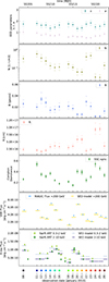 |
Fig. 9. Parameter evolution for the expanding blob model. The markers and error bars have the same meaning as in Fig. 5. |
6.2. Emission region size, bulk magnetic field, and integrated particle density evolution
Conical expansion has been observed for the source BL Lac in radio frequencies by Casadio et al. (2021). We fitted our emission region radius versus time to test for such a geometry. Figure 10 shows the expansion of the emitting region size for the expanding blob model, which agrees well with the conical jet expansion geometry proposed by Tramacere et al. (2022) studying the radio-γ delay for Mrk 421. Converting between the observer and blob frame timescales, tobs = tblob(1 + z)/δ, we fitted the temporal evolution of R with the following equation:
 (11)
(11)
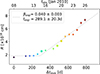 |
Fig. 10. Temporal evolution of the radius of the emitting region (R) under the expanding blob model fit with Eq. (11) using scipy curvefit. The colour key and the markers are the same as in Fig. 7. |
where ℋ is the Heaviside function and time is in the blob frame. The fit suggests a cylindrical profile up to 15 January and a subsequent conical expansion starting texp ∼ 290 days from the reference in the blob frame. The blob expansion velocity thus obtained, βexp = 0.040 (log10(βexp)∼ − 1.39), is compatible with the log10(βexp) = − 1.89 ± 0.59 reported in Tramacere et al. (2022). Additionally, our value for R0 = 1.81 × 1016 cm is compatible with the log10(R0obs)≥15.67 ± 0.59 reported by the authors, with their flat posterior distribution of the MCMC indicative of a lower limit on the parameter. In Fig. 10 we notice a hint of acceleration of blob expansion before the pile-up develops and a deceleration after the pile-up ends, the implications and consequences of which will be explored in a future work.
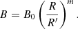
The evolution of the bulk magnetic field strength (B) versus the radius of the emission region (R) in a jet follows a power-law index assuming magnetic flux pinning and adiabatic conditions, with m = −1 for toroidal and m = −2 for poloidal bulk magnetic field configuration along the jet (Begelman et al. 1984):
 (12)
(12)
Tramacere et al. (2022) found the index, m, to be  for adiabatic blob expansion for Mrk 421. Our expanding blob model recovers a compatible index of m ∼ −1.1 for the January flare (Fig. 11), which is also consistent with the striking parsec scale toroidal magnetic field structure reported by Kovalev et al. (2025) for the blazar PKS 1424+240. However, one must note that in Tramacere et al. (2022), the authors mathematically linked B and R via Eq. (12) such that R and the index, m, were the free parameters of their model, while in our work, R and B are independent parameters. In this work, the B versus R index thus arises only as a consequence of the time evolution of the best fit to the SEDs in the expanding blob model.
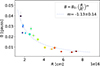 |
Fig. 11. B vs R index fit for the expanding blob model done using scipy curvefit. m = −1.13, B0 = 8.0mG, and R′ = 5.9 × 1016 cm. The colour key and markers are the same as in Fig. 7. |
Similarly, we computed the index for N versus R in Fig. 12 with the same functional form as Eq. (12), with the index being ∼ − 1.7 which indicates that there is significant particle injection; otherwise, one would expect an index of −3 for pure adiabatic expansion with no particle injection or escape. In the context of the adiabatic expansion model presented in Tramacere et al. (2022), our average spectral slope, s ∼ 1.65, is also in agreement with the EED index of  reported by the authors.
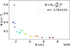 |
Fig. 12. N vs R index fit for the expanding blob model. m = −1.75, N0 = 0.067 cm−3, and R′ = 5.0 × 1016 cm. The colour key and markers are the same as in Fig. 7. |
6.3. Particle cooling timescales
We investigated the adiabatic cooling timescales for the expanding blob model and compared them with the synchrotron cooling timescales using the methodology reported in Tramacere et al. (2022). The adiabatic cooling timescale, tadiabatic ∼ R(t)/βexpc (Longair 2011), is independent of particle Lorentz factor and was computed using the expansion velocity, βexp = 0.038c, obtained in the fit to Eq. (11). On the other hand, the synchrotron cooling rate increases with the particle Lorentz factor.
Once the emission region starts to expand, the magnetic field strength drops and the synchrotron cooling timescales get longer and longer. In our model, electrons less energetic than a Lorentz factor of ∼105 have much longer synchrotron cooling timescales compared to the adiabatic cooling timescale (see Fig. 13), which is of the order of ∼150 days in the blob frame. γ ∼ 105 is also of the same order as γc and γ3p, which implies that curvature in the EED might come from a combination of stochastic acceleration and adiabatic cooling once the expansion starts after texp ∼ 290 days in the blob frame (14–15 January in the observer frame).
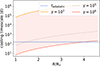 |
Fig. 13. Comparison of the particle cooling timescales (in blob frame) up to an expansion factor of ∼4.5 found in our expanding blob model, for a range of Lorentz factors. The shortest timescale for a given Lorentz factor determines the dominant mechanism for cooling. |
Given the phenomenology reported above, we conclude that the pile-up might be triggered by the sudden expansion of the blob as it travels along the jet. However, a more robust analysis using self-consistent temporal evolution is necessary to make stronger statements regarding the origin of the pile-up and the transitions between the acceleration and cooling dominated states during the multiple flaring events.
6.4. VLBI knots as expanding blobs propagating along the jet
There were two radio knots, K1 and K2, reported during 2010–2011 with a potential ejection time window in agreement with the giant flare in February. We computed the observed apparent velocity of the emission region based on the Doppler factor from our model and compared the values to the Very Long Base line Interferometry (VLBI) angular distances and the apparent radio knot velocities described in Jorstad et al. (2017), Abe et al. (2025).
Unlike K2, the existence of K1 cannot be robustly confirmed (Jorstad et al. 2017; Abe et al. 2025). The apparent velocity of knot K2 was determined to be βapp ∼ 0.3. Given the large uncertainty of the knot emission time (∼300 days for K2), it is possible that the VHE emission region and the radio knots are completely unrelated. Nevertheless, under the assumption that K2 is associated with the high-energy flare, the jet viewing angle (θview) must be very close to zero, θview ≤ 0.02°, to replicate the high Doppler beaming factor of 45 that we found necessary to capture the broadband SED. BL Lac-type objects typically have a viewing angle of ∼0° −5° and an extremely small value is statistically unlikely for Mrk 421, the closest BL Lac (Blasi et al. 2013).
Despite these caveats, we estimated the distance travelled by the blob over the ∼20 day flare (in the observer frame), amounting to ∼15 parsec for θview ∼ 0° (see Appendix D.3 and Fig. D.4). This gives an approximate distance scale along the jet over which the physical properties of the emitting region must vary (radius, magnetic field, etc.). Finally, we note that it is possible that we observe combined emission from multiple different emission regions travelling at a high bulk factor close to the base of the jet and then decelerating as they travel farther, or via a stationary shock much closer to the smbh.
7. Summary and conclusions
We processed the January 2010 MWL data of Mrk 421 to produce a sequence of SEDs. This dataset was then modelled and tested for different underlying EEDs in a single emission zone scenario. We found the phenomenology to be consistent with stochastic acceleration, independent of the EED used in our model through the trend between the synchrotron peak frequency and the peak curvature.
The standard LPPL distribution (nLPPL) works well as a first approximation. The peak position and curvature parameters are consistent with an acceleration-dominated phase of a flare and the trend of anti-correlation seen in the UV–X-ray data. However, the model fails to capture the nuanced shape of the synchrotron peak on 15, 19, and 20 January 2010, with these dates aligning with a decrease in the X-ray flux which probes the leptons with the strongest cooling. Since the LPPL distribution appears in an acceleration-dominated phase of the evolution of the particle population, this hints at a transition to a cooling-dominated phase of evolution, which we tested with a pile-up distribution (npile − up). We found that the pile-up model improved the fits on these 3 days at a TS > 4 level. The synchrotron peak of these three SEDs also has increased curvature, in agreement with theoretical work and numerical simulations of EED evolution under stochastic acceleration in the literature.
Based on the results of these fits, we found hints of expanding emission region in the evolution of the emission region parameters irrespective of the choice of EED and tested it using our modified sequential fitting method in the expanding blob model. The temporal evolution of the emitting region parameters R and B in the expanding blob model agrees well with the evolution predicted by the long term radio-γ delay study of Mrk 421 and the helical magnetic field structure of the blazar jet.
The snapshot analysis presented here is a step towards a fully self-consistent non-equilibrium model using the diffusion kinetic equations which will be a natural follow-up study to the models presented here as seen in Zech & Lemoine (2021) and Dmytriiev et al. (2021). The EED utilised in this work are analytical approximations of steady-state solutions to the diffusion equations including contributions from both first- and second-order Fermi-acceleration processes. The use of parametrised lepton distributions abstracts out the microphysical parameters while still capturing the evolution of the particle population which is the main driver of the flaring activity of Mrk 421 in our model.
Since our goal was to study acceleration-cooling transitions, we used a homogenous single zone model (see Banerjee et al. (2019) for an inhomogeneous emission region model of Mrk 421). More complex scenarios such as single-zone SSC with two population EED, multi-zone SSC, and pair-production cascade emission reported in MAGIC Collaboration (2020) can also replicate some features of our dataset at the cost of additional degeneracy of parameters. The increased curvature in the synchrotron peak is consistent with multi-zone or two-population models sometimes used in the literature, including replicating the hint of a narrow feature hinted at in the VHE spectrum, albeit with more assumptions in the model. Some of these scenarios are also discussed in Abe et al. (2025) in the context of the results for the full 2009–2010 observation campaign.
Our results also highlight that monitoring and deep observations of the brightest blazars is still a relevant science goal in the Cherenkov Telescope Array Observatory (CTAO) era, with higher time resolution and consistent coverage allowing for detailed analysis of the temporal evolution of the jet. Obtaining spectra at the light crossing timescale for a ∼1016 cm VHE emission region is still outside the capabilities of the current generation of IACTs, except for the rare cases of exceptionally strong flares, which restricts the amount of information one can possibly extract from the SED models without major assumptions. Matching the temporal resolution of the X-ray bands provided by space telescopes such as XMM-Newton and Imaging X-ray Polarimetry Explorer (IXPE) with the Large Size Telescopes (LSTs) of CTAO will open new windows into the theoretical understanding of blazar jets. The X-ray polarisation observations made possible by IXPE also provide new insights into the magnetic field structure of AGN jet, challenging existing theoretical understanding based on polarisation in the optical and radio bands. The successor to the Fermi telescope is also long overdue and highly relevant for constraining the IC peak of the SED. While the temporal resolution offered by Fermi-LAT was barely enough given the comparatively low fractional variability of Mrk 421 in the HE band and the IC peak being in the optimal range for VHE observations by MAGIC and VERITAS telescopes in this campaign, plenty of other sources will benefit from higher sensitivity in the mega-electronvolt to giga-electronvolt bands.
Acknowledgments
List of the main authors in alphabetical order – J. Abhir: project management, data analysis and modelling, paper drafting; A. Arbet-Engels: theoretical interpretation, modelling, paper drafting; D. Paneque: coordination of MWL data collection and processing; F. Schmuckermaier: MAGIC analysis cross-check; A. Tramacere: theoretical interpretation, modelling, paper drafting. The rest of the authors have contributed in one or several of the following ways: design, construction, maintenance, and operation of the instrument(s); preparation and/or evaluation of the observation proposals; data acquisition, processing, calibration and/or reduction; production of analysis tools and/or related Monte Carlo simulations; discussion and approval of the contents of the draft. We are grateful for the feedback provided by the anonymous referee which helped us improve the quality and readability of the paper. We would like to thank the Instituto de Astrofísica de Canarias for the excellent working conditions at the Observatorio del Roque de los Muchachos in La Palma. The financial support of the German BMFTR, MPG and HGF; the Italian INFN and INAF; the Swiss National Fund SNF; the grants PID2022-136828NB-C41, PID2022-137810NB-C22, PID2022-138172NB-C41, PID2022-138172NB-C42, PID2022-138172NB-C43, PID2022-139117NB-C41, PID2022-139117NB-C42, PID2022-139117NB-C43, PID2022-139117NB-C44, CNS2023-144504 funded by the Spanish MCIN/AEI/ 10.13039/501100011033 and “ERDF A way of making Europe”; the Indian Department of Atomic Energy; the Japanese ICRR, the University of Tokyo, JSPS, and MEXT; the Bulgarian Ministry of Education and Science, National RI Roadmap Project DO1-400/18.12.2020 and the Academy of Finland grant nr. 320045 is gratefully acknowledged. This work has also been supported by Centros de Excelencia “Severo Ochoa” y Unidades “María de Maeztu” program of the Spanish MCIN/AEI/ 10.13039/501100011033 (CEX2019-000918-M, CEX2021-001131-S, CEX2024001442-S), by AST22_00001_9 with funding from NextGenerationEU funds and by the CERCA institution and grants 2021SGR00426, 2021SGR00607 and 2021SGR00773 of the Generalitat de Catalunya; by the Croatian Science Foundation (HrZZ) Project IP-2022-10-4595 and the University of Rijeka Project uniri-prirod-18-48; by the Deutsche Forschungsgemeinschaft (SFB1491) and by the Lamarr-Institute for Machine Learning and Artificial Intelligence; by the Polish Ministry of Science and Higher Education grant No. 2025/WK/04; by the European Union (ERC, MicroStars, 101076533); and by the Brazilian MCTIC, the CNPq Productivity Grant 309053/2022-6 and FAPERJ Grants E-26/200.532/2023 and E-26/211.342/2021. J.A. acknowledges support from the Swiss National Science Foundation (SNSF) Grant 200020_197007. A.A.-E. acknowledges support from the Deutsche Forschungs gemeinschaft (DFG, German Research Foundation) under Germany’s Excellence Strategy – EXC-2094 – 390783311.
References
- Abdo, A. A., Ackermann, M., Ajello, M., et al. 2009, Phys. Rev. Lett., 103, 251101 [Google Scholar]
- Abe, K., Abe, S., Abhir, J., et al. 2025, A&A, 694, A195 [NASA ADS] [CrossRef] [EDP Sciences] [Google Scholar]
- Abe, K., Abe, S., Abhir, J., et al. 2026, ApJ, 998, 6 [Google Scholar]
- Abeysekara, A. U., Benbow, W., Bird, R., et al. 2020, ApJ, 890, 97 [NASA ADS] [CrossRef] [Google Scholar]
- Acciari, V. A., Ansoldi, S., Antonelli, L. A., et al. 2020, ApJS, 248, 29 [Google Scholar]
- Acharyya, A., Adams, C. B., Archer, A., et al. 2023, ApJ, 950, 152 [Google Scholar]
- Aleksić, J., Ansoldi, S., Antonelli, L. A., et al. 2015a, A&A, 576, A126 [NASA ADS] [CrossRef] [EDP Sciences] [Google Scholar]
- Aleksić, J., Ansoldi, S., Antonelli, L. A., et al. 2015b, A&A, 578, A22 [NASA ADS] [CrossRef] [EDP Sciences] [Google Scholar]
- Aleksić, J., Ansoldi, S., Antonelli, L. A., et al. 2016, Astropart. Phys., 72, 76 [Google Scholar]
- Arbet-Engels, A., Baack, D., Balbo, M., et al. 2021, A&A, 647, A88 [NASA ADS] [CrossRef] [EDP Sciences] [Google Scholar]
- Arbet-Engels, A., Bohdan, A., Rieger, F., Paneque, D., & Jenko, F. 2025, A&A, 702, A255 [NASA ADS] [CrossRef] [EDP Sciences] [Google Scholar]
- Baloković, M., Paneque, D., Madejski, G., et al. 2016, ApJ, 819, 156 [Google Scholar]
- Banerjee, B., Joshi, M., Majumdar, P., et al. 2019, MNRAS, 487, 845 [NASA ADS] [CrossRef] [Google Scholar]
- Barth, A. J., Ho, L. C., & Sargent, W. L. W. 2003, ApJ, 583, 134 [NASA ADS] [CrossRef] [Google Scholar]
- Becker, P. A., Le, T., & Dermer, C. D. 2006, ApJ, 647, 539 [Google Scholar]
- Begelman, M. C., Blandford, R. D., & Rees, M. J. 1984, Rev. Mod. Phys.; (United States), 56:2 [Google Scholar]
- Blasi, M. G., Lico, R., Giroletti, M., et al. 2013, A&A, 559, A75 [EDP Sciences] [Google Scholar]
- Blumenthal, G. R., & Gould, R. J. 1970, Rev. Mod. Phys., 42, 237 [Google Scholar]
- Böttcher, M. 2019, Galaxies, 7, 20 [Google Scholar]
- Boula, S., & Mastichiadis, A. 2022, A&A, 657, A20 [NASA ADS] [CrossRef] [EDP Sciences] [Google Scholar]
- Breeveld, A. A., Landsman, W., Holland, S. T., et al. 2011, AIP Conf. Ser., 1358, 373 [Google Scholar]
- Carnerero, M. I., Raiteri, C. M., Villata, M., et al. 2017, MNRAS, 472, 3789 [NASA ADS] [CrossRef] [Google Scholar]
- Casadio, C., MacDonald, N. R., Boccardi, B., et al. 2021, A&A, 649, A153 [NASA ADS] [CrossRef] [EDP Sciences] [Google Scholar]
- de Vaucouleurs, G., de Vaucouleurs, A., Corwin, Jr., H. G., et al. 1991, Third Reference Catalogue of Bright Galaxies (Springer) [Google Scholar]
- Dmytriiev, A., Sol, H., & Zech, A. 2021, MNRAS, 505, 2712 [NASA ADS] [CrossRef] [Google Scholar]
- Domínguez, A., Primack, J. R., Rosario, D. J., et al. 2011, MNRAS, 410, 2556 [Google Scholar]
- Fitzpatrick, E. L. 1999, PASP, 111, 63 [Google Scholar]
- Foreman-Mackey, D., Hogg, D. W., Lang, D., & Goodman, J. 2013, PASP, 125, 306 [Google Scholar]
- Fossati, G., Maraschi, L., Celotti, A., Comastri, A., & Ghisellini, G. 1998, MNRAS, 299, 433 [Google Scholar]
- Ghisellini, G., Tavecchio, F., Foschini, L., et al. 2010, MNRAS, 402, 497 [Google Scholar]
- Godet, O., Beardmore, A. P., Abbey, A. F., et al. 2009, A&A, 494, 775 [NASA ADS] [CrossRef] [EDP Sciences] [Google Scholar]
- Gokus, A., Wilms, J., Kadler, M., et al. 2024, MNRAS, 529, 1450 [Google Scholar]
- HI4PI Collaboration (Ben Bekhti, N., et al.) 2016, A&A, 594, A116 [NASA ADS] [CrossRef] [EDP Sciences] [Google Scholar]
- Jorstad, S. G., Marscher, A. P., Morozova, D. A., et al. 2017, ApJ, 846, 98 [Google Scholar]
- Kalberla, P. M. W., Burton, W. B., Hartmann, D., et al. 2005, A&A, 440, 775 [NASA ADS] [CrossRef] [EDP Sciences] [Google Scholar]
- Keenan, M., Meyer, E. T., Georganopoulos, M., Reddy, K., & French, O. J. 2021, MNRAS, 505, 4726 [NASA ADS] [CrossRef] [Google Scholar]
- Kovalev, Y. Y., Pushkarev, A. B., Gomez, J. L., et al. 2025, A&A, 700, L12 [NASA ADS] [CrossRef] [EDP Sciences] [Google Scholar]
- Krimm, H. A., Holland, S. T., Corbet, R. H. D., et al. 2013, ApJS, 209, 14 [NASA ADS] [CrossRef] [Google Scholar]
- Longair, M. S. 2011, High Energy Astrophysics (Cambridge, UK: Cambridge University Press) [Google Scholar]
- MAGIC Collaboration (Acciari, V. A., et al.) 2020, A&A, 637, A86 [NASA ADS] [CrossRef] [EDP Sciences] [Google Scholar]
- MAGIC Collaboration (Acciari, V. A., et al.) 2021, A&A, 655, A89 [NASA ADS] [CrossRef] [EDP Sciences] [Google Scholar]
- Massaro, E., Perri, M., Giommi, P., & Nesci, R. 2004, A&A, 413, 489 [NASA ADS] [CrossRef] [EDP Sciences] [Google Scholar]
- Massaro, E., Tramacere, A., Perri, M., Giommi, P., & Tosti, G. 2006, A&A, 448, 861 [NASA ADS] [CrossRef] [EDP Sciences] [Google Scholar]
- Mizuno, Y., Gómez, J. L., Nishikawa, K.-I., et al. 2015, ApJ, 809, 38 [Google Scholar]
- Partridge, B., López-Caniego, M., Perley, R. A., et al. 2016, ApJ, 821, 61 [Google Scholar]
- Prandini, E., & Ghisellini, G. 2022, Galaxies, 10, 35 [NASA ADS] [CrossRef] [Google Scholar]
- Ramaty, R. 1979, AIP Conf. Ser., 56, 135 [Google Scholar]
- Richards, J. L., Max-Moerbeck, W., Pavlidou, V., et al. 2011, ApJS, 194, 29 [Google Scholar]
- Roming, P. W. A., Kennedy, T. E., Mason, K. O., et al. 2005, Space Sci. Rev., 120, 95 [Google Scholar]
- Rybicki, G. B., & Lightman, A. P. 1986, Radiative Processes in Astrophysics (Wiley-VCH) [Google Scholar]
- Schlafly, E. F., & Finkbeiner, D. P. 2011, ApJ, 737, 103 [Google Scholar]
- Schlegel, D. J., Finkbeiner, D. P., & Davis, M. 1998, ApJ, 500, 525 [Google Scholar]
- Schlickeiser, R. 1984, A&A, 136, 227 [NASA ADS] [Google Scholar]
- Schlickeiser, R. 1985, A&A, 143, 431 [NASA ADS] [Google Scholar]
- Schlickeiser, R. 1989, ApJ, 336, 243 [NASA ADS] [CrossRef] [Google Scholar]
- Sliusar, V., Arbet-Engels, A., Baack, D., et al. 2019, in High Energy Phenomena in Relativistic Outflows VII, 32 [Google Scholar]
- Stawarz, Ł., & Petrosian, V. 2008, ApJ, 681, 1725 [Google Scholar]
- Tramacere, A. 2020, Astrophysics Source Code Library [record ascl:2009.001] [Google Scholar]
- Tramacere, A., Massaro, F., & Cavaliere, A. 2007, A&A, 466, 521 [NASA ADS] [CrossRef] [EDP Sciences] [Google Scholar]
- Tramacere, A., Giommi, P., Perri, M., Verrecchia, F., & Tosti, G. 2009, A&A, 501, 879 [NASA ADS] [CrossRef] [EDP Sciences] [Google Scholar]
- Tramacere, A., Massaro, E., & Taylor, A. M. 2011, ApJ, 739, 66 [Google Scholar]
- Tramacere, A., Sliusar, V., Walter, R., Jurysek, J., & Balbo, M. 2022, A&A, 658, A173 [NASA ADS] [CrossRef] [EDP Sciences] [Google Scholar]
- Urry, C. M., & Padovani, P. 1995, PASP, 107, 803 [NASA ADS] [CrossRef] [Google Scholar]
- Vaughan, S., Edelson, R., Warwick, R. S., & Uttley, P. 2003, MNRAS, 345, 1271 [Google Scholar]
- Zanin, R., Carmona, E., Sitarek, J., et al. 2013, in Proceedings, 33rd International Cosmic Ray Conference (ICRC2013): Rio de Janeiro, Brazil, 0773 [Google Scholar]
- Zech, A., & Lemoine, M. 2021, A&A, 654, A96 [NASA ADS] [CrossRef] [EDP Sciences] [Google Scholar]
Appendix A: SED plots and model parameters
The best-fit values of the parameters of the expanding blob model are listed in Table A.1
MCMC sampler results for the expanding blob model.
The remaining SEDs not shown in the main text for the combined model are included in Fig. A.1. All SEDs for the expanding blob model are included in Fig. A.2 and A.3.
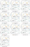 |
Fig. A.1. SED fits: combined model from 08 to 13 January, and from 21 to 26 January. Continued from Fig. 6. |
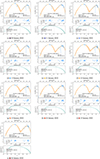 |
Fig. A.2. SED fits: expanding blob model. Similar to Fig. 6 for the expanding blob model. The best-fit value and MCMC range for the SED (top subplot) and the EED (bottom subplot) for each observation date in January 2010 are shown. The residuals of the model and the χ2, reduced χ2 ( |

Appendix B: MWL data
B.1. MAGIC VHE data
The MWL LC produced in Abe et al. (2025) was used to identify interesting flaring periods and the data from January 2010 were analysed in more detail to extract spectral points for the SEDs by integrating data into daily time bins using the standard MAGIC data reduction software MARS (Zanin et al. 2013). The daily binned spectral data points for MAGIC were processed to correct for extra-galactic background light (EBL) absorption using the Domínguez et al. (2011) model to get the intrinsic spectrum required for modelling the emission at the source.
B.2. Fermi-LAT HE data
The Fermi-LAT data were processed using fermipy v1.2 and ScienceTools v2.2.0. The low energy threshold was set to 300 MeV for the analysis as described in Abe et al. (2025) to improve the signal-to-noise ratio and angular resolution. For Fermi-LAT analysis, the TS is defined as TS = −2 ln(ℒ1/ℒ0) where ℒ1 is the likelihood of the model with the source and ℒ0 for the null hypothesis, as implemented in fermipy. We used a TS > 5 cut-off when deciding for the significance of the individual spectral points in the SED, choosing to show the 95% confidence upper-limits if the condition is not met. Despite these data quality cuts, we still have large error bars in the data given the relatively low flux of Mrk 421 compared to Fermi-LAT sensitivity.
B.3. Swift-XRT X-ray data
We analysed the curvature in the spectral points of Swift-LAT since conclusions from our stochastic model rely on accurate estimation and modelling of curvature in the synchrotron peak. Given that Mrk 421 is an extra-galactic source and outside the galactic plane of the Milky-way (J2000 Galactic coordinates 179.83 +65.03), the correction due to X-ray interactions with the atomic nH is small, and in the preliminary analysis, this effect was ignored. However, the fact that the uncertainty in nH column density estimation can mimic additional curvature in the spectrum via energy-dependent absorption of X-rays, further analysis was carried out to estimate this energy-dependent systematic uncertainty. It was found that the bins close to ∼0.5 keV were affected by higher uncertainties in the column density of galactic nH along the line of sight to the source. For getting an estimate of the increased uncertainty, nH = 1.34 × 1020 cm−2 from the 2D HI4PI map (HI4PI Collaboration 2016) and nH = 1.94 × 1020 cm−2 (Kalberla et al. 2005) were used as reference and this resulted in a maximum systematic uncertainty of ∼16% in the first two bins of the FermiXRT spectrum. Spectral bins at energies higher than ∼0.5 keV are largely unaffected by this and have the standard instrument uncertainty of 10% (Godet et al. 2009).
B.4. Swift-UVOT UV data
The Swift-UVOT provides simultaneous measurements with Swift-XRT in the UV and optical bands (Roming et al. 2005). Observations in the UVW1, UVM2, and UVW2 bands (2600 Å, 2246 Å, 1928 Å central filter wavelengths, respectively) were conducted and the data were processed using standard photometry on the total exposure for each filter band in HEAsoft v6.23. Data affected by unstable satellite attitude and from starlight of UMa 51 were filtered out. Apertures of 5 arcsec were used for the source region in each filter and ∼3 regions of 16 arcsec radius were used for the background estimation. Official calibrations from the CALDB release 20201026 were applied to the dataset (Breeveld et al. 2011) and subsequently the data were de-reddened to account for extinction (Fitzpatrick 1999; Schlafly & Finkbeiner 2011; Schlegel et al. 1998) and converted to spectral points.
B.5. Optical R-band data
The optical band data were captured by the Whole Earth Blazar Telescope (WEBT) under the GLAST-Agile Support Program (GASP) which observes Fermi-LAT monitored blazars such that contemporaneous MWL observations are available for X-ray and HE observations. Carnerero et al. (2017) processed and corrected the data for host galaxy contamination. The flux data points thus obtained were converted to spectral points for the R-band.
B.6. Radio data
Observations at 8 GHz and 14.5 GHz (University of Michigan Radio Astronomy Observatory), 15 GHz (Owens Valley Radio Observatory), 37 GHz (Metsähovi Radio Observatory) and 230 GHz (Sub-Millimeter Array) were used as described in Aleksić et al. (2015b). The simultaneity of these observations wasn’t as good as the other bands but the variability in these bands was also small (Abe et al. 2025). The fluxes were converted to spectral points using the central band frequency and the closest available observation for each radio telescope was used in the daily binned SEDs.
Appendix C: SED fits and parameter evolution
A comparison of the fits at the synchrotron peak on 15 and 20 January can be seen in Fig. C.1, showing a similar short-coming of the LPPL model in replicating the observed curvature as seen in Fig. 4.
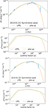 |
Fig. C.1. A comparison of the pile-up and LPPL models with a zoomed inset of the SED focused at the synchrotron peak. |
As opposed to the comparison of the LPPL and pile-up models for the same day shown previously, the evolution of the best fit of the SED and the corresponding EED around the pile-up states can be seen in Fig. C.2 and C.3.
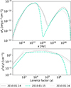 |
Fig. C.2. The evolution of spectrum and the particle population around the pile-up on 15 January. The LPPL states are plotted in black colour, and the pile-up colour key is the same as the rest of the paper. |
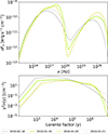 |
Fig. C.3. Evolution of the SED and EED around the pile-up states of 19 and 20 January, similar to Fig. C.2. |
The pile-up model parameter evolution can be seen in Fig. C.4. The MCMC SED fits for the expanding blob model can be seen in Fig. A.2 and A.3.
 |
Fig. C.4. Evolution of the best-fit values of the parameters for the pile-up model. The markers and error bars have the same meaning as in Fig. 5. |
Appendix D: Phenomenology - additional context and plots
D.1. Dependence of  on γ3p
As described in Sect. 5.1,  has a quadratic dependence on γ3p as long as B and δ are constants. Since our models have the bulk magnetic field as a free parameter while the beaming factor is fixed (δ = 45), the scatter in the trend in Fig. D.1 is entirely due to variations in B, resulting in a index of m = 1.23 ± 0.24 instead of m = 2.
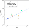 |
Fig. D.1. Combined model: Synchrotron peak position ( |

D.2. IC scattering regime
The ratio of the IC/SSC and synchrotron peak frequencies ( /
/ ) can be used to identify whether the IC scattering is in the elastic Thomson regime which works well as an approximation at lower energies or the energy dependent cross-section of the KN regime which applies at higher energy of the scattering electron. The synchrotron (under the δ approximation of synchrotron emission) and IC peak frequencies (in hertz) can be approximated as follows (Rybicki & Lightman 1986; Blumenthal & Gould 1970):
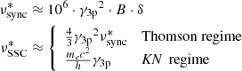
where B is in Gauss, mec2 is the rest mass of the electron and h is the Planck constant. The results from the combined model are shown in D.2, with δ = 45 and the minimum and maximum values of B obtained in the modelling used for the dashed and dotted blue lines. During January 2010, Mrk 421 has γ3p ∼ 105 − 106 such that the IC scattering is in the KN regime.
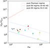 |
Fig. D.2. Combined model: Ratio of |


D.3. Expanding blob model
The expanding blob model shows very similar trends and phenomenology as the combined model. The anti-correlation of curvature as a signature of stochastic acceleration is shown in Fig. D.3. A plot of the emission region radius R versus distance from the SMBH can be seen in Fig. D.4.
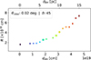 |
Fig. D.4. Expanding blob model: The expansion of the blob vs the distance from the SMBH (dBH) assuming that it is a moving emission region with a constant Doppler beaming factor δ = 45 and a viewing angle θview = 0.02° as described in Sect. 6. The blob travels about 15 parsec under these assumptions over ∼20 days. |
All Tables
Significance of the pile-up vs the LPPL EED model, with the days that have statistic (TS) > 4 (p-value < 0.05) highlighted in darker text. The TS is the likelihood ratio of the models. is the reduced-χ2, where the numerator is the χ2 and the denominator is the number of degrees of freedom of the model. The 3 days that satisfy the TS threshold for pile-up are marked with a star marker, ‘✸’, on the phenomenology plots in Sects. 5 and 6, and Appendix D.
All Figures
|
Fig. 1. VHE and X-ray LC of Mrk 421 during the 2009–2010 MAGIC observation campaign. The data were daily binned and taken from Abe et al. (2025). Our broadband SED modelling was performed over the period highlighted with a vertical red band (January 2010). Figure 2 shows the MWL data in the highlighted region in more detail. |
| In the text | |
|
Fig. 2. MWL LC during January 2010 from radio to VHE. The data were taken from Abe et al. (2025). The top axis is marked with a date colour key, which is consistent across the plots and tables in the paper. |
| In the text | |
|
Fig. 3. Anti-correlation between the peak curvature (bsync) vs the log10 of the peak frequency ( |
| In the text | |
|
Fig. 4. Comparison of the synchrotron peak of the SED and the EED of the LPPL and pile-up models on 19 January. The top panel illustrates the optical-to-X-ray SED using the pile-up (orange line) and LPPL (dashed green line) EED on 19 January 2010, the day with the strongest indication of a pile-up (see Sect. 4). The bottom panel presents the corresponding EED, where n(γ) is the particle number density distribution. The full frequency range of this SED model can be seen in Fig. 6(i). |
| In the text | |
|
Fig. 5. LPPL model results. The marker with the error bar represents [0.15, 0.50, 0.85] quantiles of 104 MCMC realisations and the short horizontal dashes represent the [0.01, 0.99] quantile range. |
| In the text | |
|
Fig. 6. SED fits: Combined model. The best fit and MCMC range for the SED (top subplot) and the EED (bottom subplot) for each observation date in January 2010 are shown. The residuals of the model and the χ2, reduced χ2 ( |
| In the text | |
|
Fig. 7. Lepton distribution curvature (r3p) at the Lorentz factor of leptons emitting at the peak of the synchrotron bump (γ3p). The fit highlights the trend between spectral curvature and peak energy for the sub-sample of days with LPPL EED in the combined model, with the pile-up states in a separate cluster at much higher curvature as predicted by the theory. The colour key is the same as Table 3 and the star markers ‘✸’ are the pile-up states. |
| In the text | |
|
Fig. 8. Trend for the synchrotron peak frequency vs peak flux, with the fit done for the overall dataset as well as excluding the pile-up states. The colour key and markers are the same as in Fig. 7. |
| In the text | |
|
Fig. 9. Parameter evolution for the expanding blob model. The markers and error bars have the same meaning as in Fig. 5. |
| In the text | |
|
Fig. 10. Temporal evolution of the radius of the emitting region (R) under the expanding blob model fit with Eq. (11) using scipy curvefit. The colour key and the markers are the same as in Fig. 7. |
| In the text | |
|
Fig. 11. B vs R index fit for the expanding blob model done using scipy curvefit. m = −1.13, B0 = 8.0mG, and R′ = 5.9 × 1016 cm. The colour key and markers are the same as in Fig. 7. |
| In the text | |
|
Fig. 12. N vs R index fit for the expanding blob model. m = −1.75, N0 = 0.067 cm−3, and R′ = 5.0 × 1016 cm. The colour key and markers are the same as in Fig. 7. |
| In the text | |
|
Fig. 13. Comparison of the particle cooling timescales (in blob frame) up to an expansion factor of ∼4.5 found in our expanding blob model, for a range of Lorentz factors. The shortest timescale for a given Lorentz factor determines the dominant mechanism for cooling. |
| In the text | |
|
Fig. A.1. SED fits: combined model from 08 to 13 January, and from 21 to 26 January. Continued from Fig. 6. |
| In the text | |
|
Fig. A.2. SED fits: expanding blob model. Similar to Fig. 6 for the expanding blob model. The best-fit value and MCMC range for the SED (top subplot) and the EED (bottom subplot) for each observation date in January 2010 are shown. The residuals of the model and the χ2, reduced χ2 ( |
| In the text | |
 |
Fig. A.3. SED fits: expanding blob model. Continued from Fig. A.2. |
| In the text | |
|
Fig. C.1. A comparison of the pile-up and LPPL models with a zoomed inset of the SED focused at the synchrotron peak. |
| In the text | |
|
Fig. C.2. The evolution of spectrum and the particle population around the pile-up on 15 January. The LPPL states are plotted in black colour, and the pile-up colour key is the same as the rest of the paper. |
| In the text | |
|
Fig. C.3. Evolution of the SED and EED around the pile-up states of 19 and 20 January, similar to Fig. C.2. |
| In the text | |
|
Fig. C.4. Evolution of the best-fit values of the parameters for the pile-up model. The markers and error bars have the same meaning as in Fig. 5. |
| In the text | |
|
Fig. D.1. Combined model: Synchrotron peak position ( |
| In the text | |
|
Fig. D.2. Combined model: Ratio of |
| In the text | |
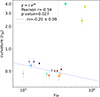 |
Fig. D.3. Expanding blob model: Anti-correlation between r3p and γ3p similar to Fig. 7. |
| In the text | |
|
Fig. D.4. Expanding blob model: The expansion of the blob vs the distance from the SMBH (dBH) assuming that it is a moving emission region with a constant Doppler beaming factor δ = 45 and a viewing angle θview = 0.02° as described in Sect. 6. The blob travels about 15 parsec under these assumptions over ∼20 days. |
| In the text | |
Current usage metrics show cumulative count of Article Views (full-text article views including HTML views, PDF and ePub downloads, according to the available data) and Abstracts Views on Vision4Press platform.
Data correspond to usage on the plateform after 2015. The current usage metrics is available 48-96 hours after online publication and is updated daily on week days.
Initial download of the metrics may take a while.