


| Issue |
A&A
Volume 710, June 2026
|
|
|---|---|---|
| Article Number | A344 | |
| Number of page(s) | 15 | |
| Section | Interstellar and circumstellar matter | |
| DOI | https://doi.org/10.1051/0004-6361/202558433 | |
| Published online | 26 June 2026 | |
A cross-match-free method for large-scale 3D extinction mapping with Gaia and 2MASS
1
Université Marie et Louis Pasteur, CNRS, Institut UTINAM, équipe Astro,
25000
Besançon,
France
2
Université de Toulouse, IRAP, CNRS, UT, CNES,
31027
Toulouse,
France
★ Corresponding author: This email address is being protected from spambots. You need JavaScript enabled to view it.
Received:
5
December
2025
Accepted:
26
April
2026
Abstract
Context. 3D extinction mapping procedures of the Milky Way face a fundamental trade-off: Gaia’s precise astrometry and photometry enable high-resolution mapping, but only to limited distances due to visible-wavelength extinction; meanwhile infrared (IR) surveys such as 2MASS penetrate deeper into the Galactic plane but provide poor distance constraints, especially in the solar neighbourhood. Many studies have cross-matched these surveys to provide more wavelength coverage and, hence, better extinction estimates. This comes at a cost as the cross-matching limits depth to the visible survey’s reach since highly extinguished stars detected in IR lack visible counterparts.
Aims. We developed PyRedLine as an evolution of the REDLINE method, enabling simultaneous exploitation of multiple surveys without cross-matching. Our goal is to achieve both high spatial resolution at short distances through Gaia and extended the reach into the Galactic plane through 2MASS, with a target resolution of ~100 pc within several kpc.
Methods. PyRedLine compares statistical distributions of observed stellar properties (colours, parallaxes, and absolute magnitudes) against predictions from the Besançon Galaxy Model reddened by parameterised extinction profiles. Using Bayesian inference with Markov chain Monte Carlo (MCMC) sampling, we can independently determine the extinction along each LOS by fitting the model predictions to Gaia DR3 and 2MASS observations simultaneously and then assembling these profiles into 3D maps. Our validation based on synthetic data confirmed a reliable structure detection out to ~8 kpc.
Results. We successfully mapped the Galactic plane from 240° ≤ l ≤ 303° and |b| ≤ 5° at 15′ resolution. The resulting map reveals extinction to 13 kpc with up to 42 pc resolution. We recovered known structures, including the Vela molecular complex and Carina arm tangent, achieving a significantly finer resolution at short distances, compared to REDLINE, while maintaining a comparable depth. We detected distant features potentially associated with the Perseus arm that remain undetected in other surveys.
Key words: methods: statistical / dust, extinction / ISM: structure / Galaxy: structure
© The Authors 2026
 Open Access article, published by EDP Sciences, under the terms of the Creative Commons Attribution License (https://creativecommons.org/licenses/by/4.0), which permits unrestricted use, distribution, and reproduction in any medium, provided the original work is properly cited.
This article is published in open access under the Subscribe to Open model. This email address is being protected from spambots. You need JavaScript enabled to view it. to support open access publication.
1 Introduction
Our position within the Milky Way (MW) offers us the possibility to study our Galaxy in great detail and to better understand stellar formation and galaxy evolution. However, it also makes the study of its structure particularly challenging because of stellar crowding and interstellar dust in the Galactic disc.
The interstellar extinction effect might stand as a major problem for observers, however, it is particularly useful in tracing dust structures. By preferentially scattering and absorbing short wavelengths, dust makes stars appear redder than their intrinsic colours to an observer, to an extent that is proportional to the dust column density along the line of sight (LOS). Interstellar extinction can therefore be used to infer the location and the dust density of interstellar clouds. Coupling this approach with stellar distance measurements makes it possible to map the position of interstellar clouds in three dimensions (3D)and, thus, to obtain an overview of the dust distribution in a vast part of the Milky Way and thereby highlighting its structure.
The first 3D extinction map can be attributed to Fernie (1962), which covers the first kiloparsec (kpc) region around the Sun. This map was very coarse, showing a dusty structure of ~500 pc in its extent. Fitzgerald (1968) provided a far more detailed map, covering 2.5 kpc around the Sun. The development of large photometric surveys, such as 2MASS (Skrutskie et al. 2006), has been a key step for devising 3D dust maps. Thanks to 2MASS, Marshall et al. (2006) managed to obtain what was the most precise and deep 3D extinction map of the Milky way, extending up to 10 kpc from the Sun. Since then, numerous 3D extinction mapping techniques have been proposed. The methods reported in Sale et al. (2014) and Guo et al. (2021) cover the northern and southern Galactic plane, respectively. Many of the recent methods rely on Gaia (Gaia Collaboration 2016, 2023) for its unprecedented precision on photometry and astrometry of about two billions of stars. However, each of these methods comes with its advantages and disadvantages. Those published by Lallement et al. (2019); Leike & Enßlin (2019); Leike et al. (2020); Dharmawardena et al. (2024); Edenhofer et al. (2024) do have pc-scale spatial resolutions, but they do not probe further than 3 kpc around the Sun. The methods of Chen et al. (2019); Green et al. (2019); Vergely et al. (2022) demonstrate a capacity to probe dust up to 4 to 6 kpc from the Sun, at the cost of a coarser spatial resolution. Since the publication of the work by Marshall et al. (2006), only a few recent methods (Cornu et al. 2022; Rezaei et al. 2024; Zucker et al. 2025; Marshall et al. 2025) have been shown to probe dust all the way to 10 kpc from the Sun.
Most of the aforementioned methods cross-matched Gaia data with other surveys, making use of parallaxes and maximising the wavelength coverage, allowing for better constraints and a relatively large distance coverage. Unfortunately, since extinction is more severe in the visible domain than in the IR, cross-matching surveys in different spectral domains limits the reach of the map to that of the shortest wavelength survey, especially in the direction of dense structures. The four methods capable of detecting structures up to 10 kpc have only used IR data, namely: APOGEE-2 in Rezaei et al. (2024), 2MASS in Marshall et al. (2006), Cornu et al. (2022) and Marshall et al. (2025), as well as a cross-match between DECaPS2 and VVV, 2MASS, unWISE, and Gaia DR3 (parallaxes only) in Zucker et al. (2025). The ability to combine multiple surveys, without cross-matching, leverages all the information from each survey, potentially increasing the distance range and the precision of a 3D extinction map.
In most studies, the motivation to cross-match surveys comes from the need to build a catalogue of stars where the distance and extinction are known for each star individually, so that photometric IR data alone (e.g. in the case of 2MASS) cannot be exploited. The strategy developed by Marshall et al. (2006), Cornu et al. (2022) and Marshall et al. (2025) (hereafter, the ‘BGM-based’ strategy) stands out by leveraging a stellar population synthesis model: the Besançon Galaxy model (BGM, Robin et al. 2003). In this approach, the information on distance is obtained statistically, typically via the colour distribution; therefore, it is free of the need to compute the distance of each star individually. The method consists of comparing the statistical distribution of stellar observable quantities (colour, magnitude, etc.) from observations and from the BGM, assuming that the differences are solely due to interstellar extinction. The 3D distribution of interstellar dust is tuned until the synthetic distributions reproduce the observed distributions tightly. Although it is a key asset to exploit IR data that probe the Galaxy deeper than visible ones, so far, only the 2MASS data were analysed with this method. Meanwhile, there is a wealth of information that is, in principle, available from Gaia with about four times more stars and parallax measurements.
The work by Cornu et al. (2022) shows that a convolutional neural network (CNN) can be employed within a BGM-based strategy to estimate the dust distribution along a LOS, thereby producing 3D extinction maps. However, training the CNN proved computationally expensive, restricting its application to a fraction of the Galactic disc between ℓ = 257° and 303°. REDLINE is another per LOS and BGM-based method that was developed by Marshall et al. (2025) to map the extinction distribution within the entire Galactic plane at |b| ≤ 1° using only 2MASS photometric data and the BGM. In contrast to the approach taken by Cornu et al. (2022), these authors relied on a Markov chain Monte Carlo(MCMC) algorithm to infer the dust distribution rather than a CNN. Their map reaches distances up to 10 kpc, with a distance binning of 100 pc and angular resolution of 10′. This work aims to demonstrate the feasibility of generalising the REDLINE method to take advantage of various, complementary surveys with heterogeneous types of data (colours, parallaxes, ...), and different stellar samples covering different distance ranges without cross-matching them. We present a new version of the method developed in python, PyRedLine. We tested it on the case of the combination of 2MASS and Gaia data without cross-match: first on synthetic data to characterise the behaviour of the new method and then on real data in a sector of the Galactic disc from ℓ = 240 deg to 303 deg.
The paper is organised as follows. We briefly summarise the data used in this work in Sect. 2. We then present our 3D extinction mapping technique in Sect. 3 and discuss its performance on synthetic data in Sect. 4. In Sect. 5, we present the results of our method applied to a region of the Galactic plane and discuss its capabilities to identify structures already identified with other methods, as well as new ones.
2 Data
In this study, we restricted ourselves to the use of Gaia DR3 and 2MASS data, both of which are all-sky surveys that are complementary in terms of wavelength coverage. Here, we present our selection criteria for both surveys and an overview of the version of the Besançon Galaxy model used in this study, as well as a description of how it was operated to generate Gaia and 2MASS stellar catalogues.
2.1 Observational data
The Two Micron All Sky Survey (2MASS) is a ground-based survey that produced uniformly calibrated observations of the entire sky in the three near-infrared (NIR) bands J (1.23 μm), H (1.66 μm), and Ks (2.16 μm). The Gaia space mission observed the entire sky in the visible domain from 2014 to 2025. The full astrometric solution of its third Data Release (DR3) contains parallaxes and photometric measurements for about 1.5 billion sources in GBP (511 nm), G (621 nm) and GRP (776 nm). For both 2MASS and Gaia DR3 photometric bands, we adopted the reference wavelengths from the SVO Filter Profile Service (Rodrigo et al. 2024).
We first selected photometric data from the 2MASS point source catalogue by choosing sources with measurements in all three bands, as well as Gaia DR3 sources with photometric measurements in all the three bands and with a parallax measurement. Then, comparing observations to a model, we needed to determine the completeness of observations for a given LOS to apply the same magnitude cuts on the observations and the model. For each photometric band of a survey, we estimate the probability density function of the magnitude using a kernel density estimator and define the completeness limit as the magnitude corresponding to the peak of this distribution. In practice, for a catalogue on n stars, each with a magnitude, x, we used a kernel density estimator based on a Gaussian kernel,
![Mathematical equation: $\[\hat{f}_h(x)=\frac{1}{n h \sqrt{2 \pi}} \sum_{i=1}^n \exp \frac{\left(x-x_i\right)^2}{2 h^2},\]$](/articles/aa/full_html/2026/06/aa58433-25/aa58433-25-eq1.png) (1)
(1)
with h as the smoothing parameter and ![Mathematical equation: $\[\hat{f}_{h}(x)\]$](/articles/aa/full_html/2026/06/aa58433-25/aa58433-25-eq2.png) is computed every 0.05 mag over the entire magnitude range of the catalogue. We used the GAUSSIAN_KDE function from the statistical module of scipy (Virtanen et al. 2020) as the (Gaussian) kernel density estimator, which automatically computes h based on the data. The completeness is used to apply magnitude cuts on observational data. Finally, we build a reliable sample by keeping only 2MASS sources with 10 ≤ Ks ≤ 16 mag and photometric errors below 0.05 mag in J, H, and Ks. For Gaia sources, we only kept the sources with 5 ≤ G ≤ 20 mag, with photometric errors below 0.05, 0.02, and 0.05 mag in GRP, G, and GBP, and with a relative error on parallaxes below 20%. We combined data from 2MASS and Gaia without any cross-match to benefit from the advantages of each survey, as explained in Sect. 3.
is computed every 0.05 mag over the entire magnitude range of the catalogue. We used the GAUSSIAN_KDE function from the statistical module of scipy (Virtanen et al. 2020) as the (Gaussian) kernel density estimator, which automatically computes h based on the data. The completeness is used to apply magnitude cuts on observational data. Finally, we build a reliable sample by keeping only 2MASS sources with 10 ≤ Ks ≤ 16 mag and photometric errors below 0.05 mag in J, H, and Ks. For Gaia sources, we only kept the sources with 5 ≤ G ≤ 20 mag, with photometric errors below 0.05, 0.02, and 0.05 mag in GRP, G, and GBP, and with a relative error on parallaxes below 20%. We combined data from 2MASS and Gaia without any cross-match to benefit from the advantages of each survey, as explained in Sect. 3.
2.2 Simulated data
The Besançon Galaxy Model is a stellar population synthesis model that simulates the stellar content of the MW statistically. This model is a tool to constrain evolutionary scenarios of the MW or to constrain the Galactic structure, such as dust distribution, by comparing model predictions to observations. The BGM versions used in Marshall et al. (2025) and the present study differ in several aspects. First, the new version used here is based on density laws determined from dynamical self-consistency using a specific galactic potential, as described by Robin et al. (2022) with a disc warped with a function derived by Chrobáková et al. (2020) from Gaia data, while Marshall et al. (2025) used the previous density model as described in Robin et al. (2003), with a warp and flare described in Lagarde et al. (2017). The second difference concerns the stellar models. Marshall et al. (2025) used STAREVOL (Lagarde et al. 2012) evolutionary tracks in the mass range from 0.7 to 6 solar masses, Baraffe et al. (1997) below 0.7, and PARSEC (Chen et al. 2015) above six solar masses, while this study uses PARSEC (Nguyen et al. 2022; Costa et al. 2025) tracks instead, between 0.1 and 120 solar masses. Our BGM version uses IMF and SFR from Mor et al. (2019), while Marshall et al. (2025) uses the IMF from Czekaj et al. (2014) and thin disc’s SFR following an exponential decrease with an exponent of 0.12 based on Aumer & Binney (2009). Lastly, this version uses the BT-Setll AGSS2009 stellar atmosphere models (Asplund et al. 2009) instead of BaSeL 3.1 (Westera et al. 2002) used by Marshall et al. (2025). For a comparison between simulated and observed distributions of stellar properties, we refer to Robin et al. (2022).
To properly compare observational data with the model, we need to apply the selection criteria to the model similar to those applied to observational data. We derived an error law for each photometric band in 2MASS and Gaia, as well as for Gaia parallaxes. Following Robin et al. (2003), we defined the error laws as
![Mathematical equation: $\[\sigma(x)=A+\exp (B \times x-C),\]$](/articles/aa/full_html/2026/06/aa58433-25/aa58433-25-eq3.png) (2)
(2)
where x is the magnitude in the considered band, while A, B, C are free parameters. We adjusted the error law based on the running median of the magnitude-uncertainty diagram for each band. We fixed A = σ(x0), the first value of the running median, while B and C are adjusted through a χ2 reduction. For Gaia parallaxes, we used a G-σϖ diagram because parallax uncertainties are correlated to a much greater extent with the G band than with the parallaxes themselves.
The BGM is set to generate stars up to 30 kpc from the Sun. The BGM is run on a grid of the plane of the sky shifted by half the desired angular resolution compared to the map discretization, as explained in Sect. 4.1. The 2MASS and Gaia mock catalogues are based on the same BGM catalogue, with one independent realisation per LOS. We considered a resolution for binaries separation of 6″ and 0.4″ for 2MASS and Gaia, respectively. The 2MASS and Gaia BGM catalogues only contain magnitudes up to 0.5 mag above the completeness of the observations. This small margin makes room for a correct generation of errors while reducing catalogues sizes and computational costs.
The Gaia Catalogue of Nearby Stars (GCNS, Gaia Collaboration 2021) contains only stars within 100 pc around the Sun. These stars are barely affected by extinction. The GCNS can then be directly compared to catalogs simulated with the BGM without considering extinction effects. Figure 1 displays the distribution of absolute magnitude, MG, versus the BP-RP between the GCNS and a simulated catalogue. The BGM accurately reproduces the observations, although the largest differences appear in the tail of the main sequence (MG > 7 mag). This is not an issue, as these stars are low-mass stars that quickly become too faint to be detected by Gaia and 2MASS at further distances.
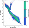 |
Fig. 1 Distribution of MG versus BP-RP for stars in a radius of 100 pc around the Sun. Filled contours: GCNS for BP < 16, G < 15, RP < 13 mag, ϖ > 10 mas. Only stars with photometric measurement in all photometric bands are represented. Magnitude cuts were computed following the procedure described in Sect. 2.1. Red contours: BGM simulated catalogue of stars using similar magnitude and parallax cuts as those of the GCNS. Photometric and parallax errors were applied on all simulated stars based on the GCNS catalogue, following the procedure described in Sect. 2.2. |
3 PyRedLine
Here, we present a PYthon based 3D REDdening mapping technique from independent LINE of sight (PyRedLine), which is an evolution of the REDLINE 3D extinction mapping technique by Marshall et al. (2025). In brief, the problem parametrisation was slightly changed to only infer the amount of extinction at predetermined distances. The Bayesian scheme was updated to use both 2MASS and Gaia photometry, as well as Gaia parallaxes. Finally, a more robust MCMC algorithm is now used to estimate the most probable dust distribution along a LOS so that the distributions of observations and model stars agree.
3.1 Problem parameters
For a given LOS, the problem is parametrised by a set of N differential extinction values ![Mathematical equation: $\[\left\{\delta A_{i}\right\}_{i=1}^{N}\]$](/articles/aa/full_html/2026/06/aa58433-25/aa58433-25-eq4.png) arranged on a distance grid. The total amount of extinction at a given distance, dn, from the observer is then given by
arranged on a distance grid. The total amount of extinction at a given distance, dn, from the observer is then given by
![Mathematical equation: $\[A(d_n)=\sum_{i=1}^n \delta A_i \delta d_i,\]$](/articles/aa/full_html/2026/06/aa58433-25/aa58433-25-eq5.png) (3)
(3)
where δdi is the distance step between point i − 1 and i, and n ∈ [1, N]. To define this distance grid, we need to estimate the maximum extinction and distance of the profile. The maximum extinction ![Mathematical equation: $\[A_{0}^{max}\]$](/articles/aa/full_html/2026/06/aa58433-25/aa58433-25-eq6.png) is estimated by comparing the 95th percentile of the colour of observed stars to the median colour of model stars, such that
is estimated by comparing the 95th percentile of the colour of observed stars to the median colour of model stars, such that
![Mathematical equation: $\[A_0^{max}=\frac{(X-Y)_{o b s}^{95}-(X-Y)_{m o d e l}^{50}}{C_X / C_Y-1},\]$](/articles/aa/full_html/2026/06/aa58433-25/aa58433-25-eq7.png) (4)
(4)
where X and Y are 2MASS or Gaia photometric bands and CX, CY are conversion coefficients to convert from A0 (541.4 nm) to AX and AY. These coefficients are derived from the Fitzpatrick et al. (2019) extinction law, with a total-to-selective extinction ratio, RV = A(V)/E(B − V), set to 3.1.
To estimate the maximum distance, the stars from the model are reddened by the extinction, ![Mathematical equation: $\[A_{0}^{max}\]$](/articles/aa/full_html/2026/06/aa58433-25/aa58433-25-eq8.png) , of a cloud located at a null distance. As a consequence, the faintest stars fall below the assumed sensitivity of the modeled survey and are dropped. Using the remaining stars, we set the maximum distance, dmax, as the 95th percentile of their distances.
, of a cloud located at a null distance. As a consequence, the faintest stars fall below the assumed sensitivity of the modeled survey and are dropped. Using the remaining stars, we set the maximum distance, dmax, as the 95th percentile of their distances.
Then, ![Mathematical equation: $\[A_{0}^{max}\]$](/articles/aa/full_html/2026/06/aa58433-25/aa58433-25-eq9.png) and dmax were used to apply a linearly increasing extinction profile to the model. The distance grid is then defined such that at least 30 stars from this reddened model fall in each distance bin. By adjusting the number of stars within the distance bins, we impose a total number of grid points (parameters) greater than 6 to avoid an overly coarse distance resolution, but below 40 to avoid an overly time-consuming CPU computation. We note that the lower limits of six points could lead to less than 30 stars per distance bin. In practice, this was never the case, as we used a denser BGM catalogue for each LOS, as explained in Sect. 4.1.
and dmax were used to apply a linearly increasing extinction profile to the model. The distance grid is then defined such that at least 30 stars from this reddened model fall in each distance bin. By adjusting the number of stars within the distance bins, we impose a total number of grid points (parameters) greater than 6 to avoid an overly coarse distance resolution, but below 40 to avoid an overly time-consuming CPU computation. We note that the lower limits of six points could lead to less than 30 stars per distance bin. In practice, this was never the case, as we used a denser BGM catalogue for each LOS, as explained in Sect. 4.1.
When using multiple surveys at once, ![Mathematical equation: $\[A_{0}^{max}\]$](/articles/aa/full_html/2026/06/aa58433-25/aa58433-25-eq10.png) and dmax are taken as the highest values among all surveys. This still leads to different distance grids because the stars detected by the various surveys are distributed differently with distance. Therefore, we concatenate and sort by distance the Gaia and 2MASS distance grids to form a single distance grid made of M values. As M can be superior to 40, we reduce the number of grid point to N = M/2, while keeping the same distance distribution of the concatenated grid. This is achieved by first smoothing the concatenated distance grid using a Gaussian kernel, which gives a distance grid d = [d0, d1, ..., dM–1]. Each grid point, di, is associated with a normalised coordinate, xi = i/(M − 1), for i = 0, 1, ..., M − 1. We then defined a reduced set of coordinates
and dmax are taken as the highest values among all surveys. This still leads to different distance grids because the stars detected by the various surveys are distributed differently with distance. Therefore, we concatenate and sort by distance the Gaia and 2MASS distance grids to form a single distance grid made of M values. As M can be superior to 40, we reduce the number of grid point to N = M/2, while keeping the same distance distribution of the concatenated grid. This is achieved by first smoothing the concatenated distance grid using a Gaussian kernel, which gives a distance grid d = [d0, d1, ..., dM–1]. Each grid point, di, is associated with a normalised coordinate, xi = i/(M − 1), for i = 0, 1, ..., M − 1. We then defined a reduced set of coordinates ![Mathematical equation: $\[x_{j}^{\prime}\]$](/articles/aa/full_html/2026/06/aa58433-25/aa58433-25-eq11.png) = j/(N − 1), with j = 0, 1, ..., N − 1, and obtained the final distance grid d′ by evaluating the linear interpolation of d(x) at the positions
= j/(N − 1), with j = 0, 1, ..., N − 1, and obtained the final distance grid d′ by evaluating the linear interpolation of d(x) at the positions ![Mathematical equation: $\[x_{j}^{\prime}\]$](/articles/aa/full_html/2026/06/aa58433-25/aa58433-25-eq12.png) .
.
3.2 Bayesian formulation
The posterior probability function of the model parameters ![Mathematical equation: $\[\theta= \left\{\delta A_{i}\right\}_{i=1}^{N}\]$](/articles/aa/full_html/2026/06/aa58433-25/aa58433-25-eq13.png) given observations O is given by Bayes’ theorem,
given observations O is given by Bayes’ theorem,
![Mathematical equation: $\[P~(\theta {\mid} O) \propto P~(O {\mid} \theta) P~(\theta).\]$](/articles/aa/full_html/2026/06/aa58433-25/aa58433-25-eq14.png) (5)
(5)
The comparison between model and observation is made via 1D or 2D histograms. We used J-K and H-K 1D histograms for 2MASS, as well as ϖ-[G-RP], ![Mathematical equation: $\[M_{G}^{\prime}\]$](/articles/aa/full_html/2026/06/aa58433-25/aa58433-25-eq15.png) -[BP-RP] 2D histograms and G-RP, BP-RP 1D histograms for Gaia, with
-[BP-RP] 2D histograms and G-RP, BP-RP 1D histograms for Gaia, with ![Mathematical equation: $\[M_{G}^{\prime}\]$](/articles/aa/full_html/2026/06/aa58433-25/aa58433-25-eq16.png) the absolute magnitude in the Gaia G band if the extinction is null. The bin widths in histograms were set following the Freedman-Diaconis rule (Freedman & Diaconis 1981), which is robust for data with outliers and for complex distributions. To ensure that the bin width is not too small compared to data errors, we set the minimum possible bin width for each histogram as the 16th percentile of the corresponding histogram colour errors. For 2MASS, we split the data in three K magnitude intervals containing the same number of stars, indirectly carrying additional information on distance. We made the J-K and H-K histograms for each interval, resulting in six different histograms for this survey.
the absolute magnitude in the Gaia G band if the extinction is null. The bin widths in histograms were set following the Freedman-Diaconis rule (Freedman & Diaconis 1981), which is robust for data with outliers and for complex distributions. To ensure that the bin width is not too small compared to data errors, we set the minimum possible bin width for each histogram as the 16th percentile of the corresponding histogram colour errors. For 2MASS, we split the data in three K magnitude intervals containing the same number of stars, indirectly carrying additional information on distance. We made the J-K and H-K histograms for each interval, resulting in six different histograms for this survey.
Following Bienayme et al. (1987), if we assume that the distribution of stars in each histogram bin, j, follows a Poisson distribution, the log-likelihood of observing O stars given that the model predicts M stars is
![Mathematical equation: $\[\ln~ P~(O {\mid} \theta)=\sum_j O_j\left[1-\frac{M_j(\theta)}{O_j}+\ln \left(\frac{M_j(\theta)}{O_j}\right)\right],\]$](/articles/aa/full_html/2026/06/aa58433-25/aa58433-25-eq17.png) (6)
(6)
The log-likelihood is only computed on histogram bins containing at least three stars to reduce noise effects. The global log-likelihood of the problem is the sum of log-likelihoods of all individual histograms.
To set the prior, we considered the following elements: (1) we expected the differential extinction values to be null when no dust was detected, but we wished to accept statistical fluctuations about zero due to noise in the observed data and because of Poisson noise. However, negative extinction being nonphysical; (2) we wish to penalise negative values beyond statistical fluctuations; and, finally, (3) we expect very high differential extinction values to be unlikely given that most 3D extinction maps (Chen et al. 2019; Green et al. 2019; Vergely et al. 2022; Dharmawardena et al. 2024; Rezaei et al. 2024; Zucker et al. 2025; Marshall et al. 2025) do not exceed 10 mag kpc−1. In cases where they do, it occurs for less than 0.1% of all cells within the Galactic plane (−1° ≤ b ≤ 1°). Thus, we defined our prior by a Gumbel Probability Density function, as it meets these three requirements:
![Mathematical equation: $\[P(\theta)=e^{-z-e^{-z}},\]$](/articles/aa/full_html/2026/06/aa58433-25/aa58433-25-eq18.png) (7)
(7)
with z = (θ − μ)/β and μ = 0. Setting β too high allows the extinction to take on large negative values, while setting it too low imposes strong penalties on high positive extinction values. After several tests on synthetic data similar to those in Sect. 4.2, and real data in the direction of Vela C (ℓ = 266.1°, b = 1°) and GRB160623A (ℓ = 84.2°, b = −2.7°, Pintore et al. 2017), β was set to 1/ max (3, γ) with
![Mathematical equation: $\[\gamma=\sum_{i=1}^N 1_{\delta A_i<0},\]$](/articles/aa/full_html/2026/06/aa58433-25/aa58433-25-eq19.png) (8)
(8)
where 1δAi<0 is the indicator function, equal to 1 when δAi < 0 and 0 otherwise.
3.3 MCMC inference
The posterior distribution is explored by MCMC to estimate the most probable dust distribution along a LOS, so the colours, parallaxes, and absolute-magnitude distributions of observation and model stars agreed. We used emcee (Foreman-Mackey et al. 2013) for the MCMC implementation. We adopted the DIME move from Boehl (2022), as it showed faster convergence for similar results compared to emcee default move (Goodman & Weare 2010) in our problem. The parameter space is explored with five times more walkers than parameters.
To initialise the walkers, we first computed the posterior of 3125 extinction profiles made from only five points. They correspond to every possibility within a distance-differential extinction space split in {1, 2, 4, 6, 10} kpc × {0, 1, 5, 15, 30} mag.kpc−1 bins. The best profile was used as the initial guess. Then, each walker was initialised by randomly drawing between one and five clouds represented by Gaussian profiles, each with a full width at half maximum (FWHM) randomly drawn between 0.25 and 1 kpc. The central position of each cloud is drawn from a pseudo probability density function corresponding to the normalised initial guess, scaled so that a cloud has between a 25–50% chance to fall where a cloud is detected on the initial guess. The scale (differential extinction) of those Gaussian clouds is drawn directly from the initial guess by linear interpolation given their positions. In addition, a random value is added to the clouds scale following a normal distribution with mean zero and standard deviation equal to the maximum differential extinction in the initial guess. This initialisation gives a great diversity to the initial values of the walkers while starting around an optimal position, allowing for a slightly faster convergence compared to a fully random initialisation. We did not identify any bias when using this scheme (as compared to a fully random initialisation scheme).
After 2000 steps, the distance grid should be redefined based on the model reddened by the median extinction profile from the last 100 steps. We computed the autocorrelation time, τf, from those 2000 iterations and ran the MCMC on this new distance grid for 50 × τf steps, which was always reached for fewer than 10 000 steps in this work. The final extinction profile corresponds to the median profile of all walkers over the last 100 steps, which is sufficient to sample the solution in the parameter space, considering the numerous walkers in our approach (Foreman-Mackey et al. 2013).
The maximum distance is only a rough estimate of the real range that can be probed during the MCMC. The last distance bins can contain too few stars to obtain reliable estimates of the dust density at such distances. To assess the significance of the furthest distance bins, we proceeded in the same way as Marshall et al. (2025), using the Bayesian information criterion,
![Mathematical equation: $\[B I C=\ln (n) k-2 ~\ln~ P(O {\mid} \theta)\]$](/articles/aa/full_html/2026/06/aa58433-25/aa58433-25-eq20.png) (9)
(9)
with k as the number of parameters, n the total number of bins in the histograms, and P(O|θ) the likelihood. We computed the BIC by removing one by one the furthest distance bins. If the BIC improved by 10 or more (Kass & Raftery 1995), we continued; otherwise, we stopped removing bins.
4 Assessment of the method
As PyRedLine is a statistical method, it is essential to assess its stability regarding the main sources of variabilities that are the BGM and the initialisation of the MCMC. Furthermore, the determination of the dust distribution in the Milky Way is a complex task, as we cannot directly compare results with direct observations of our Galaxy. It is then essential to assess the capabilities of the method to provide reliable results. With the BGM, we can create mock observations for studying the reliability of the extinction profile inferred with PyRedLine.
4.1 Uncertainties and method stability
The main sources of fluctuations between different realisations are the Poisson noise from the BGM realisation used and the initialisation of the MCMC. The contribution of the latter is already mitigated by our initialisation technique. For the former, ideally, one would require to perform multiple inferences based on different realisations of the BGM to then derive a median extinction profile, as well as uncertainties based on the scatter of the realisations. While it is tractable for single profiles, this becomes very expensive for 3D mapping. Therefore, we generated BGM catalogues on a coordinate grid shifted by half the pixel size, θ, of the map in both ℓ and b. Then, for each map LOS at Galactic coordinates l, b, the applied BGM catalogue is composed on the basis of the four nearest catalogues at l ± θ/2, b ± θ/2, leading to about a four times denser catalogue, compared to a single one. This technique slightly reduce the independence of the LOS, as BGM catalogues used to build the four times denser catalogues are shared between adjacent LOS. However, it reduces the effect of the Poisson noise on the (scaled) BGM histograms, leading to a better consistency with respect to the inference.
To investigate the method’s consistency between multiple realisations, we mapped a small region of the Galactic disc for ℓ between 257° and 303° and |b| ≤ 1°, with an angular size of 15′. This represents a total of 1472 different LOS. We compared the median of five realisations to a single realisation. We observed that the absolute median relative difference is 1.5%. The absolute median relative difference on the 16th and 84th is 1.6% and 1.7%, respectively, with a general trend of having smaller 16th and larger 84th percentiles on single realisation profiles. Furthermore, the main features are always well retrieved for single realisations and a median of multiple realisation does not remove or make appear new prominent features (i.e extinction above roughly 1 mag/kpc). This indicates a good stability on the inference whatever the BGM realisation and the MCMC initialisation. We conclude that only one realisation is sufficient when performing 3D mapping. An additional comparison between the median map from the five realisations and each individual single-realisation map is presented in Appendix A. Uncertainties on the derived extinction profile for each LOS of a 3D map were defined as the scatter of the 5 × N walkers over the last 100 MCMC iterations, which corresponds to the difference between the 84th and 16th percentiles of the parameter distribution.
4.2 Test on mock data
We tested the ability of the method to detect interstellar structures at the correct location with the correct dust density using synthetic observational data. We generated target extinction profiles as sets of Gaussian profiles, controlled by their number, size, and maximum differential extinction. These extinction profiles were used to redden the stars from an independent realisation of the BGM and errors were added to each star using the error laws derived from real data, as explained in Sect. 2.2. Finally, we discarded stars fainter than the magnitude limits determined from the observation completeness (Sect. 2.1).
4.2.1 Single cloud scenario
We tested the ability of the method to detect interstellar structures at the correct location with the correct dust density using synthetic observational data. We generated target extinction profiles as sets of Gaussian profiles, controlled by their number, size, and maximum differential extinction. These extinction profiles were used to redden the stars from an independent realisation of the BGM and errors were added to each star using the error laws derived from real data, as explained in Sect. 2.2. Finally, we discarded stars fainter than the magnitude limits determined from the observation completeness (Sect. 2.1).
A first test consisted of assessing the ability of the method to correctly localise single structures along a LOS. Figure 2 panels A, B, and C show the median profiles of cumulative extinction and differential extinction obtained from ten independent BGM realisations on synthetic data in the case of a single cloud located at 1,5 or 8.5 kpc. A single cloud is detected for all three cases, centred at ![Mathematical equation: $\[0.93_{-0.02}^{+0.03}\]$](/articles/aa/full_html/2026/06/aa58433-25/aa58433-25-eq21.png) ,
, ![Mathematical equation: $\[5.09_{-0.04}^{+0.02}\]$](/articles/aa/full_html/2026/06/aa58433-25/aa58433-25-eq22.png) and
and ![Mathematical equation: $\[8.20_{-0.11}^{+0.1}\]$](/articles/aa/full_html/2026/06/aa58433-25/aa58433-25-eq23.png) kpc in panels A, B, and C, respectively. To determine the central position of the cloud, we used a simple Bayesian framework, assuming uncertainties on the estimated extinction profile to be Gaussian-distributed. We note that the grid resolution is 0.13, 0.12 and 0.13 kpc in panels A, B, and C, which is around four times higher than the uncertainties of the cloud central position estimates of case A and B. Compared to the target distances, clouds in A and B are then well positioned via PyRedLine. The most distant cloud (panel C), is shifted by −0.3 kpc compared to the target position. This is a significant difference compared to the target position, although it remains compatible at the 2σ level, given both the grid resolution or the uncertainty on the central position. Those observations for cloud distances also apply for the width and density of the 2 closest clouds, whose widths and scale are compatible with their targets. The most distant cloud is clearly detected, but with a larger width and lower scale compared to the cloud target characteristics. We also note higher uncertainties on the differential and cumulative extinction profiles around and after the position of this cloud.
kpc in panels A, B, and C, respectively. To determine the central position of the cloud, we used a simple Bayesian framework, assuming uncertainties on the estimated extinction profile to be Gaussian-distributed. We note that the grid resolution is 0.13, 0.12 and 0.13 kpc in panels A, B, and C, which is around four times higher than the uncertainties of the cloud central position estimates of case A and B. Compared to the target distances, clouds in A and B are then well positioned via PyRedLine. The most distant cloud (panel C), is shifted by −0.3 kpc compared to the target position. This is a significant difference compared to the target position, although it remains compatible at the 2σ level, given both the grid resolution or the uncertainty on the central position. Those observations for cloud distances also apply for the width and density of the 2 closest clouds, whose widths and scale are compatible with their targets. The most distant cloud is clearly detected, but with a larger width and lower scale compared to the cloud target characteristics. We also note higher uncertainties on the differential and cumulative extinction profiles around and after the position of this cloud.
These results highlight the ability of our method to detect single clouds along a LOS and to locate them at the correct distance. They also highlight a limit of our method at large distances, where a single clouds can be detected, but biased toward lower distances.
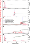 |
Fig. 2 Median extinction profile from ten independent inferences obtained with PyRedLine on synthetic observations in case of one cloud at 1 kpc (A), 5 kpc (B) and 8.5 kpc (C), two clouds (D), and three clouds (E) along the LOS. The green and blue curves are cumulative and differential target extinction profiles, respectively. The black curve and red stepped curve represent the median cumulative and differential extinction profiles estimated by PyRedLine, respectively. Shaded regions correspond to the interval between the 16th and 84th percentiles of the last 100 MCMC steps of all the walkers from the ten inferences. |
4.2.2 Multiple cloud scenarios
Another particularly interesting text consisted of assessing the capabilities of the method to identify distant structures behind dense regions. Panels D and E of Fig. 2 show the median profiles of cumulative extinction and differential extinction for synthetic data in the case of two low density clouds at 5 and 8.5 kpc (D) and three clouds at 1,5, and 8.5 kpc (E) along the LOS.
The first detected cloud in panel D is located at the correct distance, at ![Mathematical equation: $\[5.01_{-0.05}^{+0.05}\]$](/articles/aa/full_html/2026/06/aa58433-25/aa58433-25-eq24.png) kpc, while this same cloud is detected at
kpc, while this same cloud is detected at ![Mathematical equation: $\[5.10_{-0.09}^{+0.09}\]$](/articles/aa/full_html/2026/06/aa58433-25/aa58433-25-eq25.png) kpc in panel E. The presence of the first dense cloud degrades the detection of the second cloud in panel E, with PyRedLine placing it 100 pc too far. The furthest cloud is detected at
kpc in panel E. The presence of the first dense cloud degrades the detection of the second cloud in panel E, with PyRedLine placing it 100 pc too far. The furthest cloud is detected at ![Mathematical equation: $\[7.92_{-0.12}^{+0.13}\]$](/articles/aa/full_html/2026/06/aa58433-25/aa58433-25-eq26.png) kpc and
kpc and ![Mathematical equation: $\[8.78_{-0.12}^{+0.17}\]$](/articles/aa/full_html/2026/06/aa58433-25/aa58433-25-eq27.png) kpc in panels D and E, respectively. It corresponds to shifts of −0.58 kpc in panel D and +0.28 kpc in panel E compared to the cloud target distance. Although this cloud seems to be better located in panel E, it is only slightly detected and is very elongated, with a far larger apparent width than the target width of 800 pc.
kpc in panels D and E, respectively. It corresponds to shifts of −0.58 kpc in panel D and +0.28 kpc in panel E compared to the cloud target distance. Although this cloud seems to be better located in panel E, it is only slightly detected and is very elongated, with a far larger apparent width than the target width of 800 pc.
These results indicate that our method seems robust at short and medium distances, even in the case of multiple clouds along the LOS. However, it can struggle at large distances, potentially detecting clouds at a wrong distance and/or with an incorrect width and/or differential extinction. This appears to be the results of the combination of three factors: measurement errors, weak long-distance constraints due to a coarse resolution of 2MASS histograms (examples of histograms are presented in Appendix B), and distance grid-induced bias due to large distance steps at large distances. The presence of multiple clouds along the LOS can exacerbate this problem. Thus, even if our method is able to detect far away structures at distances greater than 8 kpc, their distance estimates must be considered with caution.
5 The Vela-Carina region
We applied our method to map the Vela-Carina region defined at a Galactic longitude between ℓ = 240° and 303° and Galactic latitude |b| ≤ 5 degrees. This choice is motivated by the presence in this region of small- and large-distance structures; mainly, the Vela molecular complex (VMC), the tangent of the Carina arm, and the extremity of the Perseus arm. We sampled the region using 10 080 independent LOS, with an angular resolution of 15′. All LOS profiles were interpolated onto a common distance grid with 42 pc resolution, corresponding to the highest spatial resolution among all LOS. Computing this map required a total of ~100k CPU hours using heterogeneous processors1.
5.1 Single and combined survey mapping
PyRedLine can infer dust distribution using only a single survey or by combining several surveys. Figure 3 shows three maps obtained with PyRedLine using only Gaia, only 2MASS, and the combination of both surveys. While the use of 2MASS alone leads to a systematic overestimation of dust density for distances below 500 pc, Gaia tends to correct it. As expected, short distance structures are much more constrained thanks to Gaia, such as the VMC at 257° < ℓ < 272°, with structures that closely match the location of young open clusters (YOC, age < 20 Myr) from Hunt & Reffert (2023), HII regions from Hou & Han (2014) and molecular clouds from Miville-Deschênes et al. (2017). This is the case for most of the main structures up to 6 kpc, after which the remaining structures can mainly be identified thanks to 2MASS.
Overall, the similarities between the position of the different tracers and the detected structures is good in all three cases, except for ℓ > 287°. In this sector, the maps reveal highly dispersed structures with low to moderate differential extinction, while the few known tracers do not coincide with any prominent features. In particular, the region between 2 and 5 kpc appears to correspond to a void in the tracer distribution. The group of HII regions at (ℓ ~ 290°, d ~ 8 kpc) does not have a dense counterpart in our map. The other HII group at (ℓ ~ 298°, d ~ 10 kpc) has a weak and elongated counterpart in the 2MASS-only map, but not in the Gaia map. This is expected, as Gaia detects very few stars at such distances. However, when combining both surveys, this HII group falls into what appears to be a cavity in our map. The structure that was primarily detected with 2MASS at a similar distance as this HII groups gets pushed to 12 kpc and it is less elongated and slightly denser. Whether this is the result of a better constraint thanks to Gaia or of a bias it introduces is uncertain. However, the disagreement between our map and the tracers for this structure is in favor of the second possibility.
The most noticeable addition of 2MASS is the structure C behind the VMC, which has not been detected using Gaia data alone. While the feature extending from ℓ = 240° and d ~ 6 kpc to ℓ = 278° and d ~ 9 kpc appears as a single, continuous structure on the 2MASS-only maps (whose two halves are denoted as B′ and C in Fig. 3, middle frame), Gaia data make it easier to resolve it, splitting it into structures A and B at lower longitudes (ℓ < 256°, Fig. 3, lower frame), once there are no more dense foreground structures. Additionally, from the Gaia+2MASS map, structure B may extend behind Vela to a distance of approximately 10 kpc, but cannot be identified as such due to the very high dust density of the VMC. Another possibility is that structure C represents the unresolved continuation of structures A and B beyond ℓ > 256°.
However, the difference between the 2MASS-only map and the Gaia+2MASS map in the apparent continuity of B′ and C across a wide range of Galactic longitudes raises concerns about their reliability. The morphology of B appears strongly correlated with that of A. While structure A is consistently observed in both the Gaia-only and combined maps, structure B emerges distinctly strictly on the combined map. This suggests that B primarily originates from 2MASS and might be caused by structure A displacing B′ to greater distances. These observations suggest that structures B could be an artefact, whereas structure A remains plausible. This is supported by our analysis of the spread (uncertainty) of the combined map in Appendix C.
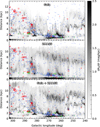 |
Fig. 3 Extinction map of the Vela-Carina region for |b| ≤ 1° in Cartesian coordinates. The maps were obtained with PyRedLine using either only Gaia, only 2MASS, or the combination of both. Red squares are HII region from Hou & Han (2014), with the sizes proportional to the excitation parameter. Blue circles are molecular clouds from Miville-Deschênes et al. (2017), with sizes proportional to the column density of clouds. Green triangles are young open clusters (Age < 20 Myr) from Hunt & Reffert (2023), with sizes proportional to the number of star members. Markers A, B, B’, and C highlight remarkable structures. |
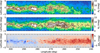 |
Fig. 4 Comparison between the Planck dust opacity map and PyRedLine. Top: Planck τ353 map converted in A0. Middle: integrated extinction map obtained by combining Gaia and 2MASS. Bottom: difference between PyRedLine and Planck map. Contours correspond to Planck τ353 = 0.00008, 0.00016 and 0.00028. |
5.2 Comparison with Planck
The Planck dust optical depth (PDOD) (Planck Collaboration XLVIII 2016) can be considered as a good proxy of the interstellar dust distribution integrated along the LOS, although the authors did report some limitations, especially near the Galactic plane. We converted the PDOD map at τ353 to extinction in A0 from a fit of the correlation between our extinction map and the PDOD map, restraining the fit to |b| > 3°, where the PDOD map is expected to be the most reliable. We found a conversion law given by A0 = ατ353, with α = 4.3 × 10⁴ mag.
Figure 4 shows the PDOD map converted to extinction, the integrated extinction map obtained with PyRedLine and the difference ΔA0 between PyRedLine and Planck maps. Most of the structures highlighted by the contours from the Planck map can be identified in our extinction map. Our method retrieves both high-density and low-density structures with morphologies that are very similar to those visible on the Planck map. However, differences can be observed, with the most prominent one being a strong large-scale gradient in ΔA0 along Galactic longitude, PyRedLine finding more dust as we get closer to the Galactic anti-centre. For 240° < l < 278° and −2.5° < b < 2°, the median overestimation by PyRedLine is +3.6 mag. In contrast, for ℓ > 280°, PyRedLine tends to detect less dust, with a median underestimation of −3.04 mag. The region at ℓ < 278 appears significantly denser in the PyRedLine map compared to the PDOD map. This corresponds to the longitude range where the structures A, B, and C are observed in Fig. 3 (see Appendix D).
We discarded from our 3D extinction map the region that corresponds to the structures A, B, and C, for d ≥ 5 kpc. With this region removed, the updated conversion factor becomes α = 3.3 · 104 mag, representing a 23% decrease compared to the initial value. Figure 5 presents a revised comparison between the PyRedLine integrated extinction map and the PDOD map, following the exclusion of the region associated with structures B and C, as well as part of A. The improvement is remarkable. The large-scale gradient in ΔA0 along Galactic longitude is no longer present. For −2.5° < b < 2° and 240° < l < 278°, the median overestimation by PyRedLine is reduced to +0.08 mag, while it is of +0.37 mag for ℓ > 280°. This slightly larger value originates from the significant extinction overestimation by PyRedLine towards the Carina tangent (281 ≤ ℓ ≤ 288). The highest values of ΔA0 are mainly observed towards dense regions.
There are several effects that might contribute to the differences that are still observed in Fig. 5. Since dust is practically optically thin in the far-IR FIR domain, Planck can detect dust emission from much larger distances than Gaia and 2MASS can detect stars. This can explain underestimations in our map compared to Planck. Then, the PDOD map can suffer from biases linked to gradients in dust temperature along the LOS (Planck Collaboration XLVIII 2016), which can lead to underestimating dust opacity in the PDOD map. Another contribution may be that we used a constant RV value for the extinction law in PyRedLine. Since RV is known to increase in dense regions, it can lead to an overestimated extinction in our map.
This comparison to the PDOD indicates that features B and C are probably artefacts. The foreground part of structure A, up to 5 kpc, might be part of a real structure, as its presence improves the agreement of the PyRedLine integrated extinction map with the PDOD map. However, the remaining part of A, at distances larger than 5 kpc, could be an artefact, similarly to B and C. We discuss the reliability of these structures in Sect. 5.6 with all the other available elements. The remaining features of the map appear to be reliable, such as those corresponding to the VMC, or towards the Carina arm tangent. An additional comparison with the Planck dust temperature map is presented in Appendix F.
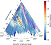 |
Fig. 6 Polar view of the Vela-Carina region for |b| < 1°, overlaid with spiral arm models from Reid et al. (2019) as a solid line, Hou (2021) as a dotted line, and Marshall et al. (2025) as a dashed-dotted line. The Carina arm is in magenta, the Perseus arm in black, and the Norma-Outer arm in red. Reid et al. (2019) and Hou (2021) models have been extrapolated. |
5.3 Spiral arm identification
High extinction regions correspond to dense and massive regions of the ISM that are closely associated with star forming regions. Galactic spiral arms stand out by their intense star formation activity, making interstellar dust a good tracer of spiral arms. Our map covers a region of the Galactic plane that intercepts parts of the Carina and the Perseus arms (Vallée 2008).
Figure 6 displays logarithmic spiral arm models from Reid et al. (2019) (R19), Hou (2021) (H21) and Marshall et al. (2025) (M25) on top of a polar view of the median dust distribution within the Vela-Carina region. The R19 model is adjusted on maser parallaxes, while the H 21 model is adjusted on measured distances of giant molecular clouds, masers, HII regions, O-type stars, and YOCs. The M25 model is adjusted on their 3D extinction map. R19 model barely covers the Vela-Carina region and requires extrapolation, as for H21 that partially covers it. In contrast, the M25 model fully covers the Vela-Carina region.
As expected, the elongated structure at 282° < ℓ < 285° and d ~ 4 kpc corresponds to the tangent of the Carina arm, in agreement with all models. The structure close to 12 kpc at ℓ > 298 is potentially part of this arm as well, with a fair agreement with the R19 model, especially when considering that the distance to this structure might be overestimated (Sect. 5.1).
Using the models from R19 and M25, we identify structure C (see Fig. 3) to what could correspond to the extremity of the Perseus arm. The H21 model, which is adjusted using tracers primarily located in the solar neighbourhood, can exhibit biases at greater distances. This appears to be the case here, as the H 21 model for the Perseus arm deviates from R19 and M25 models, as well as from the position of feature C on our map.
However, spatial alignment alone does not confirm that feature C is a real structure and the match might be the result of a coincidence. Similarly, structure B could correspond to the extremity of the Outer arm given R19 model, although it is slightly shifted towards larger distances. Structure A, which is more reliable than structures B and C (see Sect. 5.2), appears to coincide with the Perseus arm.
If, by any means, structure B and C are real features, PyRedLine would then be the first 3D extinction mapping technique to detect components of the Perseus and Outer arms within this region of the MW. Nonetheless, in the absence of corroborating evidence, such a conclusion remains speculative. We return to the reliability of structure A, B, and C in Sect. 5.6.
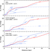 |
Fig. 7 Comparison of the cumulative extinction as a function of the distance between this work (D26, red solid), M25 (blue dashed), Z25 (blue dash-double-dotted), V22 (blue dashed-dotted), CO22 (blue dotted), and CH19 (blue dense dash-dotdotted) towards three lines of sight in the Galactic plane at (ℓ, b) = (270°, −0.5°) (top), (282°, −0.75°) (middle), and (301°, 0.25°) (bottom). |
5.4 Comparison with other works
Probing dust at large distance is challenging and only small number of studies have managed to detect Galactic structures further than 5 kpc from the Sun. Figure 7 compares cumulative extinction profiles obtained by this work (D26), M25, Zucker et al. (2025) (Z25), Cornu et al. (2022) (CO22), Vergely et al. (2022) (V22) and Chen et al. (2019) (CH19), for three LOSs through the VMC (ℓ, b) = (270°, −0.5°), the tangent of the Carina arm (ℓ, b) = (282°, −0.75°), and near the edge of our map (ℓ, b) = (301°, 0.25°). The Fitzpatrick et al. (2019) (F19) extinction law with RV = 3.1 was used to convert M25 and CO22 from AV to A0 (this conversion also depends on the source spectrum, an effect neglected here), Z25 from E(B − V) to A0, and CH19 to A0 based on the provided conversion E(B − V) = 0.75 × E(GBP − GRP).
For the LOS through Vela, our method mainly follows V22 up to its distance limit of 5 kpc. Afterwards, we find a similar morphology than M25, but slightly shifted toward higher extinction. All methods agree at ~6 kpc, except CH19, which diverges from all other methods after 0.8 kpc (i.e. at the Vela location). Z25 detects Vela at a shorter location than D26, M25, V22, and CH19, while CO22 detects it even more closely. We detected the first structure along the tangent of the Carina arm at a slightly larger distance than the other methods, although with a somewhat similar density as in M25. Furthermore, CH19, V22, and Z25 did not appear to detect any clear structure after 4 kpc, while D26, M25, and CO22 detected important dust quantities. We note the very good agreement of D26, M25 and CO22 near 4.5 kpc, as well as an overall good agreement between this work and M25. Finally, CO22 seems to systematically detect structures at shorter distance for this LOS. For the LOS at (ℓ, b) = (301°, 0.25°), all the maps are in strong agreement at 2 kpc, except CO22. M25, Z25, and D26 are in agreement once again at 5.5 kpc; afterwards, we closely followed Z25 to reach a similar level as CO22.
Figure 8 shows a qualitative comparison of polar views representing the median dust distribution in a region of the Galactic disc at 240° < ℓ < 303°, up to 13 kpc, for this work, as well as M25 and Z25 (see as well Appendix E). The most noticeable differences lie in the presence of the three structures A, B, and C in our map, with B and C potentially corresponding to the Outer and Perseus arms, as outlined in Sect. 5.3; however, we note that they might be artefacts, as suggested following the comparison to the PDOD map detailed in Sect. 5.2, and further discussed in Sect. 5.6. Features B and C are not visible in Z25. CO22 shows only a faint detection near 6 kpc for 258 ≤ ℓ ≤ 275. Despite also using 2MASS data (i.e. the BGM and a similar methods), M25 does not reveals the presence of the structures B and C. Some foreground components of structure A appear on M25 and Z25 maps, mainly around 4 kpc at ℓ ≈ 243°, 255° and 258°. This supports the interpretation that the foreground part of A might be reliable. However, they appear far more prominently on the PyRedLine map. Z25 scarcely identified any structures along the tangent of the Carina arm at d > 4 kpc, whereas in the present work, M25 and CO22 did identify them. The structure we observed at ℓ = 282°, d = 8 kpc seems to better correspond with the overdensity at 6 kpc on M25 and 7 kpc on CO22. Furthermore, for this same structure, M25 and CO22 show a better match with HII regions, suggesting that our estimated distance of 8 kpc might be overestimated. The same observation can be performed for the structure at ℓ > 296°, d = 12 kpc, detected at 10 kpc in CO22 and M25, again showing a better alignment with HII regions. Those structures, shifted by 2 kpc compared to M25 and CO22, may indicate a potential distance bias in our method for some structures at large distances. This is consistent with the outcome of our analysis on synthetic data in Sect. 4.2.2, where we suggested that PyRedLine yields the most reliable results up to 8 kpc.
5.5 Comparison with HI and H2
Söding et al. (2025) (S25) constructed spatially coherent 3D density maps of HI and H2 across the entire MW, using 21-cm HI data from the HI4PI full-sky survey (HI4PI Collaboration 2016) and CO (J = 0 → 1) emission data from Dame et al. (2001) and Dame & Thaddeus (2022). Figure 9 presents the superposition of S 25 HI (top) and H2 (bottom) distributions in the form of contours onto our extinction map.
We note a good alignment between our map and the distribution of H2 for the VMC, the Carina complex and the different structures towards the Carina tangent up to 6 kpc. The structure at ℓ ~ 300°, d = 2.5 kpc appears to have a counterpart in the H2 distribution. This is not the case for structure A, B, and C.
The alignment between our extinction map and S25 HI map is less pronounced. This is somewhat expected, as HI does not necessarily correlate with dust. However, we expect large scale (~1 kpc) HI and dust distributions to be somewhat correlated. Here, Structure B does not align well with the distribution of HI. Surprisingly, the best match appears to be for structures A and C. It reinforces the reliability of structure A, and suggests that feature C may not be an artefact, or at least not entirely. Therefore, the nature of structure C is called into question.
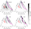 |
Fig. 8 Polar view of the dust distribution in a region Galactic plane at 240° < ℓ < 303° and |b| < 1° from this work, Z 25, M25, and CO22 up to 13 kpc. Markers and spiral arms are similar to Fig. E.1. |
5.6 Discussion on structures A, B, and C
In light of the different arguments presented in previous sections, we posit that structure B could be an artefact. However, the origin of this feature remains unclear. The coarse resolution of the 2MASS histograms, combined with a possible bias from the distance grid, may contribute to the emergence of such artefacts. In addition, such features are not visible in M25, despite the use of 2MASS data, the BGM and a similar method. These observations highlight the need for further investigation to clarify the origin of such features.
The comparison between our extinction maps and the distribution of HI and HII gas assesses the large-scale distribution of dust along the LOS, whereas the comparison between our integrated extinction map and the PDOD map compares the total extinction (i.e. the total dust content) along the LOS. While these two comparisons support the reliability of the foreground component of structure A, this is not the case for its more distant parts (hereafter A-far), nor for structure C. It is plausible that A-far and C are real Galactic structure, detected at approximately correct locations, but with overestimated extinction levels. One possible explanation for such an overestimation by PyRedLine is its use of a fixed RV value of 3.1. If the true RV within a structure is higher than the value assumed by PyRedLine, the method compensates by inferring a higher amount of extinction. Conversely, if the actual RV value is lower, PyRedLine underestimates the extinction. This effect can be significant if RV deviates from 3.1 over large distances. Therefore, it might be possible that the true RV value within A-far and C (and B) exceeds 3.1, leading PyRedLine to overestimate the extinction in these regions. Unfortunately, this portion of the Galactic disc is not covered by the recent 2D RV map from Zhang et al. (2023), neither by the 3D RV map from Zhang & Green (2025) at such large distances, preventing us from verifying whether or not RV is indeed greater than 3.1 in this region. If the latter hypothesis were proven correct, we need to consider why the impact of RV would be significant only for A-far, B, and C, and not for other structures. One possibility is that RV might be even higher in A-far, B, and C than in typical molecular clouds. Yet, we have to consider what would justify such an excess. One possibility could be linked to a change in dust grains properties in those regions, as suggested by the variations of the dust temperature from Planck and discussed in Appendix F. However, in the absence of a clear explanation, these questions remain unresolved and underline the need for further investigation.
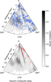 |
Fig. 9 Face-on view of the Vela-Carina region for |b| ≤ 1° in polar coordinates, up to 13 kpc from the Sun. Blue filled contours corresponds to ∑HI ≥ 5 M⊙.pc−2 (light blue) and ∑HI ≥ 8 M⊙ pc−2 (blue). Red filled contours corresponds to ∑H2 ≥ 1 M⊙ pc−2 (light red) and ∑H2 ≥ 3 M⊙ pc−2 (red). HI and H2 gas densities from Söding et al. (2025). |
6 Conclusion
We present an updated version of the REDLINE method by Marshall et al. (2025), named PyRedLine, designed to combine multiple surveys without cross matching them. The strength of this method relies on the Besançon Galaxy Model, allowing us to infer the dust distribution along any LOS using photometry and astrometry, without requiring any explicit use of distance measurements. For this proof of concept, we used 2MASS, Gaia DR3 photometry, as well as Gaia DR3 parallaxes to assess the performance of our method on synthetic and real data, mapping a region of the Galactic disc with 10080 independent LOSs at 240° ≤ ℓ ≤ 303° and |b| ≤ 5. Our main conclusions are as follows.
Using tests on synthetic data and the comparison of our results to others, we assessed the robustness of PyRedLine for 3D extinction mapping. PyRedLine is able to produce maps of intermediate angular resolution (15′), with a distance range up to 13 kpc and a variable distance resolution down to 42 pc. It allows for the detection of structures at both small and large distances with precision, making of it one of the most capable method to probe deeply into the plane of the Milky Way, which is essential to better understanding its structure.
We detected candidate structures (i.e. A and C) that could delineate a segment of the Perseus arm that had gone previously undetected in existing 3D extinction maps. In addition to the Carina arm, several inter-arm structures are clearly identifiable, showing the potential of PyRedLine for the study of the Milky Way at the level of both medium- and large-scale structures.
The method can effectively use Gaia and 2MASS data without cross-match, thanks to the use of the BGM, which provides information on distances. This allows for the detection of deep and highly reddened structures, such as structures located at large distances in the Carina arm. This is promising for the future of this method, which is capable of combining even more surveys and at different wavelengths to probe even deeper into the Galactic disc.
Discrepancies with the Planck dust optical depth map raise concerns about a possible extinction overestimation in some regions, possibly due to the unaccounted variation of RV across the Galaxy. This suggests that it might be important to incorporate spatial variations of RV into PyRedLine. In addition, the method could benefit from an improvement on the resolution of 2MASS histograms, as well as of the distance grid to improve the reliability of the method for d > 8 kpc.
The present work is focussed on pushing back the current distance limit of most 3D mapping techniques by developing a robust method to study the structure of the Milky Way at large distances. While REDLINE excels at large distances, PyRedLine seems to work at all distances and works very well at short distances, without necessarily relying on explicit distance estimates from data.
The next step is to use PyRedLine to map the entire Galactic plane for b < |1°|. Such a map will allow probing the structure of the Galactic disc up to the Galactic centre with the highest precision to date. Future improvements to the PyRedLine method are considered, starting with an improvement of the precision at very short distances. Additionally, given the high dimensionality of the problem, the use of a nested sampling algorithm, such as UltraNest (Buchner 2021), could offer significant benefits over traditional MCMC approaches.
With the next Gaia releases planned in 2026 (DR4) and 2030 (DR5), 3D dust maps will become even more precise, but not necessarily deeper. Our method will be able to take advantage of the improvement brought by those releases and use them in combination with IR surveys such as 2MASS, AllWISE, GLIMPSE, and Roman telescope surveys in the future to explore the structure of the Galactic disc as never before, possibly venturing beyond the Galactic centre.
Data availability
The 3D extinction map is available at the CDS via https://cdsarc.cds.unistra.fr/viz-bin/cat/J/A+A/710/A344.
Acknowledgements
The authors acknowledge the support of the Programme National ‘Physique et Chimie du Milieu Interstellaire’ (PCMI) of CNRS/INSU with INC/INP co-funded by CEA and CNES. This publication makes use of data products from the Two Micron All Sky Survey, which is a joint project of the University of Massachusetts and the Infrared Processing and Analysis Center/California Institute of Technology, funded by the National Aeronautics and Space Administration and the National Science Foundation. This work has made use of data from the European Space Agency (ESA) mission Gaia (https://www.cosmos.esa.int/gaia), processed by the Gaia Data Processing and Analysis Consortium (DPAC, https://www.cosmos.esa.int/web/gaia/dpac/consortium). Funding for the DPAC has been provided by national institutions, in particular the institutions participating in the Gaia Multilateral Agreement. This research has made use of the SVO Filter Profile Service “Carlos Rodrigo”, funded by MCIN/AEI/10.13039/501100011033/ through grant PID2023-146210NB-I00. Computations have been performed on computers of the Institut UTINAM of the Université Marie & Louis Pasteur, supported by the Région Bourgogne-Franche-Comté and the Institut des Sciences de l’Univers (INSU).
References
- Asplund, M., Grevesse, N., Sauval, A. J., & Scott, P. 2009, ARA&A, 47, 481 [CrossRef] [Google Scholar]
- Aumer, M., & Binney, J. J. 2009, MNRAS, 397, 1286 [NASA ADS] [CrossRef] [Google Scholar]
- Baraffe, I., Chabrier, G., Allard, F., & Hauschildt, P. H. 1997, A&A, 327, 1054 [Google Scholar]
- Bienayme, O., Robin, A. C., & Crézé, M. 1987, A&A, 180, 94 [NASA ADS] [Google Scholar]
- Boehl, G. 2022, DIME MCMC: A Swiss Army Knife for Bayesian Inference [Google Scholar]
- Buchner, J. 2021, J. Open Source Softw., 6, 3001 [CrossRef] [Google Scholar]
- Chen, Y., Bressan, A., Girardi, L., et al. 2015, MNRAS, 452, 1068 [Google Scholar]
- Chen, B.-Q., Huang, Y., Yuan, H.-B., et al. 2019, MNRAS, 483, 4277 [NASA ADS] [CrossRef] [Google Scholar]
- Chrobáková, v. Z., Nagy, R., & López-Corredoira, M. 2020, A&A, 637, A96 [NASA ADS] [CrossRef] [EDP Sciences] [Google Scholar]
- Cornu, D., Montillaud, J., Marshall, D. J., Robin, A. C., & Cambrésy, L. 2022, arXiv e-prints [arXiv:2201.05571] [Google Scholar]
- Costa, G., Shepherd, K. G., Bressan, A., et al. 2025, A&A, 694, A193 [NASA ADS] [CrossRef] [EDP Sciences] [Google Scholar]
- Czekaj, M. A., Robin, A. C., Figueras, F., Luri, X., & Haywood, M. 2014, A&A, 564, A102 [NASA ADS] [CrossRef] [EDP Sciences] [Google Scholar]
- Dame, T. M., & Thaddeus, P. 2022, ApJS, 262, 5 [NASA ADS] [CrossRef] [Google Scholar]
- Dame, T. M., Hartmann, D., & Thaddeus, P. 2001, ApJ, 547, 792 [Google Scholar]
- Dharmawardena, T. E., Bailer-Jones, C. A. L., Fouesneau, M., et al. 2024, MNRAS, 532, 3480 [Google Scholar]
- Edenhofer, G., Zucker, C., Frank, P., et al. 2024, A&A, 685, A82 [NASA ADS] [CrossRef] [EDP Sciences] [Google Scholar]
- Fernie, J. D. 1962, AJ, 67, 224 [Google Scholar]
- Fitzgerald, M. P. 1968, AJ, 73, 983 [NASA ADS] [CrossRef] [Google Scholar]
- Fitzpatrick, E. L., Massa, D., Gordon, K. D., Bohlin, R., & Clayton, G. C. 2019, ApJ, 886 [Google Scholar]
- Foreman-Mackey, D., Hogg, D. W., Lang, D., & Goodman, J. 2013, PASP, 125, 306 [Google Scholar]
- Freedman, D., & Diaconis, P. 1981, Z. Wahrsch. Verwandte Gebiete, 57, 453 [Google Scholar]
- Gaia Collaboration (Prusti, T., et al.) 2016, A&A, 595, A1 [NASA ADS] [CrossRef] [EDP Sciences] [Google Scholar]
- Gaia Collaboration (Smart, R. L., et al.) 2021, A&A, 649, A6 [EDP Sciences] [Google Scholar]
- Gaia Collaboration (Vallenari, A., et al.) 2023, A&A, 674, A1 [NASA ADS] [CrossRef] [EDP Sciences] [Google Scholar]
- Goodman, J., & Weare, J. 2010, CAMCS, 5, 65 [Google Scholar]
- Green, G. M., Schlafly, E., Zucker, C., Speagle, J. S., & Finkbeiner, D. 2019, ApJ, 887, 93 [NASA ADS] [CrossRef] [Google Scholar]
- Guo, H. L., Chen, B. Q., Yuan, H. B., et al. 2021, ApJ, 906, 47 [NASA ADS] [CrossRef] [Google Scholar]
- HI4PI Collaboration (Ben Bekhti, N., et al.) 2016, A&A, 594, A116 [NASA ADS] [CrossRef] [EDP Sciences] [Google Scholar]
- Hou, L. G. 2021, Front. Astron. Space Sci, 8, 103 [Google Scholar]
- Hou, L. G., & Han, J. L. 2014, A&A, 569, A125 [NASA ADS] [CrossRef] [EDP Sciences] [Google Scholar]
- Hunt, E. L., & Reffert, S. 2023, A&A, 673, A114 [NASA ADS] [CrossRef] [EDP Sciences] [Google Scholar]
- Kass, R. E., & Raftery, A. E. 1995, JASA, 90, 773 [CrossRef] [Google Scholar]
- Lagarde, N., Decressin, T., Charbonnel, C., et al. 2012, A&A, 543, A108 [NASA ADS] [CrossRef] [EDP Sciences] [Google Scholar]
- Lagarde, N., Robin, A. C., Reylé, C., & Nasello, G. 2017, A&A, 601, A27 [NASA ADS] [CrossRef] [EDP Sciences] [Google Scholar]
- Lallement, R., Babusiaux, C., Vergely, J. L., et al. 2019, A&A, 625, A135 [NASA ADS] [CrossRef] [EDP Sciences] [Google Scholar]
- Leike, R. H., & Enßlin, T. A. 2019, A&A, 631, A32 [NASA ADS] [CrossRef] [EDP Sciences] [Google Scholar]
- Leike, R. H., Glatzle, M., & Enßlin, T. A. 2020, A&A, 639, A138 [NASA ADS] [CrossRef] [EDP Sciences] [Google Scholar]
- Marshall, D. J., Robin, A. C., Reylé, C., Schultheis, M., & Picaud, S. 2006, A&A, 453, 635 [NASA ADS] [CrossRef] [EDP Sciences] [Google Scholar]
- Marshall, D. J., Montillaud, J., Cambrésy, L., & Cornu, D. 2025, A&A, 704, A118 [NASA ADS] [CrossRef] [EDP Sciences] [Google Scholar]
- Miville-Deschênes, M.-A., Murray, N., & Lee, E. J. 2017, ApJ, 834, 57 [Google Scholar]
- Mor, R., Robin, A. C., Figueras, F., Roca-Fàbrega, S., & Luri, X. 2019, A&A, 624, L1 [NASA ADS] [CrossRef] [EDP Sciences] [Google Scholar]
- Nguyen, C. T., Costa, G., Girardi, L., et al. 2022, A&A, 665, A126 [NASA ADS] [CrossRef] [EDP Sciences] [Google Scholar]
- Pintore, F., Tiengo, A., Mereghetti, S., et al. 2017, MNRAS, 472 [Google Scholar]
- Planck Collaboration XI. 2014, A&A, 571, A11 [NASA ADS] [CrossRef] [EDP Sciences] [Google Scholar]
- Planck Collaboration XLVIII. 2016, A&A, 596, A109 [NASA ADS] [CrossRef] [EDP Sciences] [Google Scholar]
- Reid, M. J., Menten, K. M., Brunthaler, A., et al. 2019, ApJ, 885, 131 [Google Scholar]
- Rezaei, S. K., Beuther, H., Benjamin, R. A., et al. 2024, A&A, 692, A255 [NASA ADS] [CrossRef] [EDP Sciences] [Google Scholar]
- Robin, A. C., Reylé, C., Derrière, S., & Picaud, S. 2003, A&A, 409, 523 [NASA ADS] [CrossRef] [EDP Sciences] [Google Scholar]
- Robin, A. C., Bienaymé, O., Salomon, J. B., et al. 2022, A&A, 667, A98 [NASA ADS] [CrossRef] [EDP Sciences] [Google Scholar]
- Rodrigo, C., Cruz, P., Aguilar, J. F., et al. 2024, A&A, 689, A93 [NASA ADS] [CrossRef] [EDP Sciences] [Google Scholar]
- Sale, S. E., Drew, J. E., Barentsen, G., et al. 2014, MNRAS, 443, 2907 [NASA ADS] [CrossRef] [Google Scholar]
- Skrutskie, M. F., Cutri, R. M., Stiening, R., et al. 2006, AJ, 131, 1163 [NASA ADS] [CrossRef] [Google Scholar]
- Söding, L., Edenhofer, G., Enßlin, T. A., et al. 2025, A&A, 693, A139 [CrossRef] [EDP Sciences] [Google Scholar]
- Vallée, J. P. 2008, AJ, 135, 1301 [CrossRef] [Google Scholar]
- Vergely, J. L., Lallement, R., & Cox, N. L. J. 2022, A&A, 664, A174 [NASA ADS] [CrossRef] [EDP Sciences] [Google Scholar]
- Virtanen, P., Gommers, R., Oliphant, T. E., et al. 2020, Nat. Methods, 17, 261 [Google Scholar]
- Westera, P., Samland, M., Bruzual, G., & Buser, R. 2002, in Observed HR Diagrams and Stellar Evolution, 274, 166 [Google Scholar]
- Ysard, N., Jones, A. P., Guillet, V., et al. 2024, A&A, 684, A34 [NASA ADS] [CrossRef] [EDP Sciences] [Google Scholar]
- Zhang, X., & Green, G. M. 2025, Science, 387, 1209 [Google Scholar]
- Zhang, R., Yuan, H., & Chen, B. 2023, ApJS, 269, 6 [NASA ADS] [CrossRef] [Google Scholar]
- Zucker, C., Saydjari, A. K., Speagle, J. S., et al. 2025, ApJ, 992, 39 [Google Scholar]
Intel Xeon Gold 5218R, Intel Xeon Gold 6248R, AMD EPYC 7443.
Appendix A Additional evidence of the method stability
In addition to the per LOS comparison outlined in Sect. 4.1 between a median of 5 realisations and a single realisation, we have computed the relative difference between a median map of 5 realisations, and single realisation maps. Figure A.1 shows such a comparison for 257° < ℓ < 303° and |b| < 1°. The median relative difference is −2.86%, indicating a slight underestimation in single-realisation inference maps compared to the median map. This difference highlights a strong edge effect, due to the fluctuations of the distance range that each LOS can cover at each realisation. Two other parts of the map suffer from strong fluctuations, near ℓ = 296°, 8.2 < d < 12 kpc, and 288° < ℓ < 296°, 2.1 < d < 5 kpc. Those area mainly correspond to cavities, with very little dust. Furthermore, PyRedLine systematically determines a small amount of “negative dust density” exactly and only for those two regions. Having very high fluctuations at those particular regions indicates a potential significant deviation between observational and BGM predicted star properties. Negative extinction values could arise from:
local variations in intrinsic stellar properties (e.g. metallicity, age, IMF) not considered in the model.
local deviations in stellar density distributions relative to the large-scale disc tendency.
local variations in dust properties (e.g. RV), although the precise impact of such variations on PyRedLine capability to infer negative extinction remains uncertain.
Large local fluctuations between different realisations may come from the the Poisson noise in BGM catalogues whose effect could be amplified under the conditions outlined above, particularly in regions where the extinction is very low. Further investigation is needed to draw robust conclusions about the origin of these anomalies.
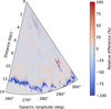 |
Fig. A.1 Median relative difference between a median map made from 5 independent realisations, and the individual maps from the 5 realisation themselves. The maps considered here are polar views representing the median dust distribution in the Galactic disc for 257° < ℓ < 303° and |b| < 1°. |
Appendix B Examples of control histograms
Figure B.1 and B.2 are examples of control histograms used to assess the quality of the results for a single LOS, here in the case of the 3-cloud test case presented in Sect. 4. All 1D BGM histograms (in red) shows very close colour distributions compared to synthetic observational histograms (in blue). The ϖ − [G − RP] and ![Mathematical equation: $\[M_{G}^{\prime}\]$](/articles/aa/full_html/2026/06/aa58433-25/aa58433-25-eq28.png) − [BP − RP] diagrams are as well similar between the reddened BGM (in red) and the observations. Those two figures clearly show that 2MASS histograms have lower resolution than Gaia histograms, which explain why 2MASS is lacking precision on the position of the detected structures compared to Gaia, mainly at short and large distances, where the small number of stars might have a minimal impact on the colour distributions due to the coarse resolution of the histograms.
− [BP − RP] diagrams are as well similar between the reddened BGM (in red) and the observations. Those two figures clearly show that 2MASS histograms have lower resolution than Gaia histograms, which explain why 2MASS is lacking precision on the position of the detected structures compared to Gaia, mainly at short and large distances, where the small number of stars might have a minimal impact on the colour distributions due to the coarse resolution of the histograms.
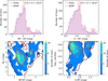 |
Fig. B.1 Gaia control histograms for the 3-cloud test case of Sect. 4. Blue shades represent observational data. Red shades represent reddened BGM data. For 2D histograms, contours correspond to 68th, 90th, 95th and 99th percentiles. |
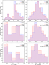 |
Fig. B.2 2MASS control histograms for the 3-cloud test case of Sect. 4. Blue shades represent observational data. Red shades represent reddened BGM data. |
Appendix C Uncertainty map
Figure C.1 shows a polar view of the dust distribution uncertainty estimate (spread) in the Galactic disc, at 240° < ℓ < 303° and b ≤ 1°. The spread is defined as the difference between the 16th and 84th percentiles. The uncertainty fluctuations mainly follow dust distribution fluctuations, with generally higher uncertainties at high dust density and/or large distances. The median signal to noise ratio is 4.2, indicating a overall good reliability of the map. This map reveals a significant spread of the walkers for structures B and C, indicating the difficulty of the method to properly constrain these regions. This indicates that the actual amount of extinction inferred for these structures is unreliable. In addition, it could suggest that structures B and C are artefacts. The spread around structure A is considerably smaller, suggesting that it is a more robust feature, at least within the latitude range |b| ≤ 1°.
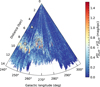 |
Fig. C.1 Averaged spread of the estimated dust distribution in the Galactic plane at 240° < ℓ < 303°, |b| < 1°. The spread is based on the 16th and 84th percentiles. Markers A, B, and C are similar to Fig. 3. |
Appendix D Integrated sliced maps
Figure D.1 presents the PyRedLine map integrated in distance slices. It strongly suggests that the overall overestimation of extinction by PyRedLine in the region ℓ ∈ [240°, 278°] is primarily due to the detection of dense structures between 4 and 10 kpc. Structures A, B and C are the main features within this longitude and distance range. In addition, the morphologies of the structures between 1 and 4 kpc in Fig. D.1 closely match with dense features identified on the PDOD map in Fig. 4.
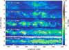 |
Fig. D.1 Integrated extinction over different distance ranges for the Vela-Carina region. |
Appendix E Additional comparison
Figure E.1 is similar to Fig. 8, but compares this work to M25, Z25, CH19, V22, and CO22 only up to 5 kpc. The morphology and dust density of the VMC (258° < ℓ < 272°, d < 3 kpc) is very similar between our work and Z25. The position of its foreground part is similar between our work and M25, V22 and CH19. Z25 starts detecting it at shorter distances, while CO22 places it further, at 1.1 kpc. The position of this foreground part in our map better matches YOC positions than Z25. Gum 10 at ℓ = 254, d = 3.3 kpc, is barely visible on CH19 map, but clearly detected by V22, M25, Z25 and D26, although with slight variations in distance. M25 detects it at slightly larger distances, at around 3.5 kpc, whereas Z25 detects it at 3 kpc, perfectly matching the 2 HII regions present at this location. The Carina complex, at 285° ≤ ℓ ≤ 289°, −2° ≤ b ≤ 1°, is detected at around 2.3 kpc on our map and matches with YOCs and HII tracers within this area. The Carina complex appears more prominently on Z25 map, but at a shorter distance of ~2.1 kpc. On the M25 map, a structure is present at this location but is significantly affected by Finger of God (FOG) artefacts. CH19 and V22 also detect the Carina complex, but as a more diffuse feature compared to Z25 and D26. CO22 suffers from substantial FOG artefacts in this region, making any conclusion ambiguous.
The foreground structure along the tangent of the Carina arm (ℓ = 282°, d = 1.6 kpc) is detected at a similar position in CH19, V22, CO22 and this work. Z25 detects this structure at a slightly shorter distance of ~1.3 kpc. It is unclear whether this structure is detected by M25, as it seems to be blended with a background structure.
While all maps show striking similarities, a few structures show completely different morphology, density and location from one map to the other. For instance, the dense structure in V22 at ℓ = 300°, d = 3.7 kpc seems to be only slightly detected in CH19, but at a similar location. CO22 finds a very dense structure at this longitude, but with a completely different shape and at around 3.3 kpc. M25, Z25 and this work all find a structure with a relatively similar shape, but with high density for Z25, medium for M25, and low for this work. Its position between M25 and this work seems relatively similar, at around 3.3 kpc, but Z25 detects it much closer, at 2.5 kpc. Drawing conclusions about the correct location of this structure is challenging, as no YOCs, HII regions of molecular clouds match with any map. However, Z25 shows a systematic shift toward shorter distances compared to the other maps, potentially indicating that this structure is not where Z25 detects it, but rather at a larger distance, between 3 and 4 kpc. We note that V22 displays fewer elongated structures than the other methods we presented. This arises from its use of a 3D Gaussian kernel, which enforces isotropic spatial correlations that other approaches do not enforce.
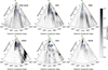 |
Fig. E.1 Polar view of the dust distribution in region of the Galactic plane at 240° < ℓ < 303° and |b| < 1° for this work, Z25, M25, CO22, V22 and CH19 up to 5 kpc. Markers are similar to Fig. 3. |
Lastly, significant differences appear between the results obtained with REDLINE and PyRedLine using only 2MASS data (c.f. Fig. 3, 8 and E.1). The variations in the first kiloparsec are mainly due to the poor sampling of the distance grid in PyRedLine below 1 kpc owing to the low stellar density in that region. Other variations may arise from the BGM version, the use of different colours (J-K and H-K in this work, J-H and H-K in M25), the resolution of 2MASS colour histograms and finally the different implementations of the MCMC methods used. Further investigations are needed to determine the exact source(s) of these differences.
Appendix F Dust temperature from Planck
The Planck dust temperature map (Planck Collaboration XI 2014) shows a remarkable change in the dust temperature around 280 degrees in longitude. This map is represented in Fig. F.1, for 240° < ℓ < 320° and b < |15°|. For ℓ < 280°, the dust is relatively hot, while it is cooler at lower longitude. The strong overestimation of the extinction from PyRedLine compared to Planck on Fig. 4 and highlighted by a red contour on Fig. F.1, appears to align with this change in dust temperature.
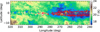 |
Fig. F.1 Planck dust temperature map from ℓ = 240° to ℓ = 320° and b ≤ |15|°. The red contour corresponds to a difference between PyRedLine and the PDOD map of A0 = 2.5 mag. |
This change in dust grain temperature appears mainly within the Galactic plane, where the mixing of different environment along the LOS complicate the interpretation. Still, one possibility for such a variation in the dust temperature could be a variation in the dust grain properties. But the properties of dust grains directly affect the extinction curve. Therefore, as the extinction curve used by PyRedLine is fixed, any deviation from it within the observations could result in an overestimation or underestimation of the extinction from PyRedLine. One way to consider these variations could be to adjust RV for each LOS. But that could be insufficient and the use of a proper dust model, such as THEMIS 2 (Ysard et al. 2024), could be needed. However, this would most likely make the method heavier, as one would need to adjust the dust model grain properties in addition to the extinction.
All Figures
|
Fig. 1 Distribution of MG versus BP-RP for stars in a radius of 100 pc around the Sun. Filled contours: GCNS for BP < 16, G < 15, RP < 13 mag, ϖ > 10 mas. Only stars with photometric measurement in all photometric bands are represented. Magnitude cuts were computed following the procedure described in Sect. 2.1. Red contours: BGM simulated catalogue of stars using similar magnitude and parallax cuts as those of the GCNS. Photometric and parallax errors were applied on all simulated stars based on the GCNS catalogue, following the procedure described in Sect. 2.2. |
| In the text | |
|
Fig. 2 Median extinction profile from ten independent inferences obtained with PyRedLine on synthetic observations in case of one cloud at 1 kpc (A), 5 kpc (B) and 8.5 kpc (C), two clouds (D), and three clouds (E) along the LOS. The green and blue curves are cumulative and differential target extinction profiles, respectively. The black curve and red stepped curve represent the median cumulative and differential extinction profiles estimated by PyRedLine, respectively. Shaded regions correspond to the interval between the 16th and 84th percentiles of the last 100 MCMC steps of all the walkers from the ten inferences. |
| In the text | |
|
Fig. 3 Extinction map of the Vela-Carina region for |b| ≤ 1° in Cartesian coordinates. The maps were obtained with PyRedLine using either only Gaia, only 2MASS, or the combination of both. Red squares are HII region from Hou & Han (2014), with the sizes proportional to the excitation parameter. Blue circles are molecular clouds from Miville-Deschênes et al. (2017), with sizes proportional to the column density of clouds. Green triangles are young open clusters (Age < 20 Myr) from Hunt & Reffert (2023), with sizes proportional to the number of star members. Markers A, B, B’, and C highlight remarkable structures. |
| In the text | |
|
Fig. 4 Comparison between the Planck dust opacity map and PyRedLine. Top: Planck τ353 map converted in A0. Middle: integrated extinction map obtained by combining Gaia and 2MASS. Bottom: difference between PyRedLine and Planck map. Contours correspond to Planck τ353 = 0.00008, 0.00016 and 0.00028. |
| In the text | |
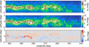 |
Fig. 5 Same as Fig. 4, but excluding structures B and C, keeping A up to 5 kpc. |
| In the text | |
|
Fig. 6 Polar view of the Vela-Carina region for |b| < 1°, overlaid with spiral arm models from Reid et al. (2019) as a solid line, Hou (2021) as a dotted line, and Marshall et al. (2025) as a dashed-dotted line. The Carina arm is in magenta, the Perseus arm in black, and the Norma-Outer arm in red. Reid et al. (2019) and Hou (2021) models have been extrapolated. |
| In the text | |
|
Fig. 7 Comparison of the cumulative extinction as a function of the distance between this work (D26, red solid), M25 (blue dashed), Z25 (blue dash-double-dotted), V22 (blue dashed-dotted), CO22 (blue dotted), and CH19 (blue dense dash-dotdotted) towards three lines of sight in the Galactic plane at (ℓ, b) = (270°, −0.5°) (top), (282°, −0.75°) (middle), and (301°, 0.25°) (bottom). |
| In the text | |
|
Fig. 8 Polar view of the dust distribution in a region Galactic plane at 240° < ℓ < 303° and |b| < 1° from this work, Z 25, M25, and CO22 up to 13 kpc. Markers and spiral arms are similar to Fig. E.1. |
| In the text | |
|
Fig. 9 Face-on view of the Vela-Carina region for |b| ≤ 1° in polar coordinates, up to 13 kpc from the Sun. Blue filled contours corresponds to ∑HI ≥ 5 M⊙.pc−2 (light blue) and ∑HI ≥ 8 M⊙ pc−2 (blue). Red filled contours corresponds to ∑H2 ≥ 1 M⊙ pc−2 (light red) and ∑H2 ≥ 3 M⊙ pc−2 (red). HI and H2 gas densities from Söding et al. (2025). |
| In the text | |
|
Fig. A.1 Median relative difference between a median map made from 5 independent realisations, and the individual maps from the 5 realisation themselves. The maps considered here are polar views representing the median dust distribution in the Galactic disc for 257° < ℓ < 303° and |b| < 1°. |
| In the text | |
|
Fig. B.1 Gaia control histograms for the 3-cloud test case of Sect. 4. Blue shades represent observational data. Red shades represent reddened BGM data. For 2D histograms, contours correspond to 68th, 90th, 95th and 99th percentiles. |
| In the text | |
|
Fig. B.2 2MASS control histograms for the 3-cloud test case of Sect. 4. Blue shades represent observational data. Red shades represent reddened BGM data. |
| In the text | |
|
Fig. C.1 Averaged spread of the estimated dust distribution in the Galactic plane at 240° < ℓ < 303°, |b| < 1°. The spread is based on the 16th and 84th percentiles. Markers A, B, and C are similar to Fig. 3. |
| In the text | |
|
Fig. D.1 Integrated extinction over different distance ranges for the Vela-Carina region. |
| In the text | |
|
Fig. E.1 Polar view of the dust distribution in region of the Galactic plane at 240° < ℓ < 303° and |b| < 1° for this work, Z25, M25, CO22, V22 and CH19 up to 5 kpc. Markers are similar to Fig. 3. |
| In the text | |
|
Fig. F.1 Planck dust temperature map from ℓ = 240° to ℓ = 320° and b ≤ |15|°. The red contour corresponds to a difference between PyRedLine and the PDOD map of A0 = 2.5 mag. |
| In the text | |
Current usage metrics show cumulative count of Article Views (full-text article views including HTML views, PDF and ePub downloads, according to the available data) and Abstracts Views on Vision4Press platform.
Data correspond to usage on the plateform after 2015. The current usage metrics is available 48-96 hours after online publication and is updated daily on week days.
Initial download of the metrics may take a while.