


| Issue |
A&A
Volume 710, June 2026
|
|
|---|---|---|
| Article Number | A321 | |
| Number of page(s) | 15 | |
| Section | Extragalactic astronomy | |
| DOI | https://doi.org/10.1051/0004-6361/202558256 | |
| Published online | 24 June 2026 | |
Discovery of new N-emitters over a wide redshift range
1
Observatoire de Genève, Université de Genève, Chemin Pegasi 51, 1290 Versoix, Switzerland
2
CNRS, IRAP, 14 Avenue E. Belin, 31400 Toulouse, France
3
Institut d’Astrophysique de Paris, UMR 7095 CNRS, Sorbonne Université, 98bis, Bd Arago, 75014 Paris, France
4
Cosmic Dawn Center (DAWN), Niels Bohr Institute, University of Copenhagen, Jagtvej 128, København N, DK-2200, Denmark
★ Corresponding author: This email address is being protected from spambots. You need JavaScript enabled to view it.
Received:
25
November
2025
Accepted:
21
April
2026
Abstract
Context. Recent James Webb Space Telescope (JWST) observations have revealed a small number of galaxies with UV spectra exhibiting intense nitrogen emission lines, which are not typically detected in galaxy spectra. The observations indicate super-solar N/O abundances at low metallicity, a phenomenon whose nature is currently intensely debated.
Aims. To better understand these enigmatic objects and provide new constraints on proposed scenarios, we did a systematic search for galaxies with UV nitrogen emission lines (N IV] λ1486 and/or N III] λ1750).
Methods. Using public JWST NIRSpec data, we identified 45 N-emitters with robust N III] or N IV] detections, including four previously known objects. We then classified these objects, determined relative C, N, O, and H chemical abundance ratios, determined other properties, and carried out a statistical analysis of the N-emitter population.
Results. We find N-emitters at redshifts z ∼ 3 − 11 spanning a broad diversity of galaxies in terms of morphology, UV magnitude, stellar mass, star formation rate, metallicity, and rest-optical emission line strengths. The UV nitrogen lines show typical equivalent widths (EW) between ∼5 Å and up to ∼100 Å in a few cases. Diverse ionisation conditions, as traced by N IV] λ1486/N III] λ1750, are observed. The carbon lines (C IVλ1550 and C III] λ1909) are generally fainter than the N lines. Using strong line calibrations established at high-redshift, we find metallicities 12 + log(O/H)∼7.15 − 8.5, spanning up to high metallicity values. The Hβ EW of N-emitters varies strongly, and sources with low EWs show clear signs of a Balmer break, indicative of composite stellar populations combining both young (≲10 Myr) stars responsible for the UV emission lines and an older population contributing to the rest-optical spectrum. Super-solar N/O ratios are found in all N-emitters. C/O abundances are comparable to those of galaxies at the same metallicity, and all N-emitters show either high N/C ratios or lower limits (log(N/C) ≳ 0.5), regardless of metallicity. The observed abundance ratios are compatible with ejecta from H-burning and show no signs of carbon enhancements, even at higher metallicities. Finally, we find that the fraction of N-emitters increases with redshift, and we quantify this evolution.
Conclusions. Our study increases the sample of known N-emitters by a factor of ∼3, reveals a diversity of properties among N-emitters, and provides new constraints on their nature.
Key words: galaxies: abundances / galaxies: high-redshift / galaxies: ISM
© The Authors 2026
 Open Access article, published by EDP Sciences, under the terms of the Creative Commons Attribution License (https://creativecommons.org/licenses/by/4.0), which permits unrestricted use, distribution, and reproduction in any medium, provided the original work is properly cited.
This article is published in open access under the Subscribe to Open model. This email address is being protected from spambots. You need JavaScript enabled to view it. to support open access publication.
1. Introduction
JWST observations have revealed an unexpected diversity of rest-frame UV emission lines in galaxies at the earliest cosmic epochs. More specifically, GN-z11 at z = 10.6 exhibits a very peculiar NIRSpec spectrum (Bunker et al. 2023), characterised by strong N IV] λ1486 and N III] λ1750 emission lines, which are very rare in typical star-forming galaxies (SFGs). Using emission line measurements, Cameron et al. (2023) derived an exceptionally high nitrogen-to-oxygen ratio for GN-z11 (log(N/O) ≳ −0.25) at such a low metallicity (12 + log(O/H)≈7.90; Álvarez-Márquez et al. 2025). This finding is at odds with standard galactic chemical evolution models and observations of low-redshift galaxies and H II regions, where the N abundance is essentially constant at low metallicities and increases only later, when the bulk of nitrogen – produced as a secondary element by intermediate-mass asymptotic giant branch (AGB) stars – comes into play (Henry et al. 2000; Kobayashi 2026). Following this discovery, a few other objects that deviate significantly from the standard N/O versus O/H relation were reported (Marques-Chaves et al. 2024; Schaerer et al. 2024; Naidu et al. 2026; Navarro-Carrera et al. 2025; Castellano et al. 2024). These and other nitrogen-enhanced galaxies now include approximately 22 objects – as compiled by Ji et al. (2026) – predominantly found at high redshift, and several metal-poor, low-z galaxies with enhanced N/O abundances have also recently been reported (see Bhattacharya & Kobayashi 2026; Martinez et al. 2025).
The newly discovered high-z objects share extreme physical properties beyond their chemical ‘anomalies’. Their C/O ratio remains surprisingly consistent with those of ‘normal’ SFGs (Marques-Chaves et al. 2024; Ji et al. 2026). They typically exhibit high electron densities (Ji et al. 2024), strong UV luminosities, and remarkably elevated surface densities of both star formation rate (SFR) and stellar mass (M★) (Schaerer et al. 2024). Furthermore, these galaxies show relatively high equivalent widths, EW(Hβ) (Topping et al. 2025), suggesting the presence of young stellar populations. These shared properties depict a compact, dense, young star-forming (SF) environment within these peculiar objects. Moreover, the detection of high N/O ratios in high-redshift galaxies suggests that the process must occur relatively rapidly.
A variety of scenarios have been proposed to explain the observed N-enhancement, including enrichment from massive star winds (Wolf-Rayet, hereafter WR stars), AGB stars and selective outflows, or possibly more ‘exotic’ scenarios such as the tidal disruption of stars from encounters with black holes, very massive star (VMS) ejecta, or even supermassive stars (SMSs) (Bunker et al. 2023; Cameron et al. 2023; Charbonnel et al. 2023; D’Antona et al. 2023; Bhattacharya & Kobayashi 2026; Vink 2023; Marques-Chaves et al. 2024; D’Antona et al. 2025; McClymont et al. 2025). However, the origin of the observed N-enrichment remains largely unanswered.
To better understand these interesting objects, larger samples and new observational constraints are needed. To do so, we used a large collection of public JWST spectra and carried out a systematic search for N-emitters, defined as galaxies showing UV N IV] λ1486 and/or N III] λ1750 emission lines. Our study significantly increases the number of N-emitters at z ∼ 3 − 10, revealing a diversity of galaxies among them and providing new insights into these enigmatic objects.
The paper is structured as follows. In Sect. 2, we describe the observational data and the new N-emitter sample. Section 3 describes the empirical and basic derived properties of the sample. We present the derived O/H metallicities, chemical abundances, and their morphological properties in Sect. 4. Finally, we discuss the surprising diversity of the N-emitter population and provide a statistical estimate of their incidence, before discussing the potential origins of the observed nitrogen enrichment (Sect. 5). Our main results are summarised in Sect. 6. Throughout this work, we assumed a concordance cosmology with Ωm = 0.3, ΩΛ = 0.7, and H0 = 70 km s−1 Mpc−1.
2. JWST observations and sample selection
To search for N-emitter candidates, we used the DAWN JWST Archive (DJA)1 database of distant galaxies, specifically the version that includes automated measurements of numerous emission lines (Brammer 2023; Heintz et al. 2025; Valentino et al. 2025; Brammer, Private Communication). We selected galaxies with reliable spectroscopic redshifts (grade = 3) and extracted all spectra where one or both of the N IV] λ1486 and N III] λ1750 UV lines are potentially detected, with a signal-to-noise ratio of S/N ≥ 3. To achieve the broadest possible spectral coverage, we used only the NIRSpec PRISM spectra, which span wavelengths of λobs ∼ 0.7 − 5.2 μm, with a resolution varying from R ≃ 30 to ≃300 across this range. Our selection covers all MSA PRISM spectra included in the DJA database up to August 18, 2025. Our preselection yields 633 automatically selected candidates.
2.1. Emission line measurements and final selection
After assessing the quality of the N IV] and N III] detections, we found several to be spurious. To obtain a more reliable estimate of the detection significance of the UV nitrogen emission lines, we remeasured their fluxes, EWs, and line widths (full width at half-maximum, FWHM) using two different approaches (Lime and a custom-made code) described in Appendix A.
We define our sample of N-emitters as sources with S/N ≥ 3 in the N IV] and/or N III] lines. This yields a total of 70 N-emitter candidates. After a detailed visual inspection of the 1D and 2D spectra by several team members, we excluded 24 additional sources from the sample, as the nitrogen lines showed significant deviations from the expected line positions, issues in the 2D spectra, and features consistent with spurious detections. Our final selection consists of 45 N-emitters, listed in Table B.1.
2.2. Spectral classification: SFG, AGN, and LRD
Our sample of 45 new N-emitters exhibits a wide range of spectral features, as highlighted in Fig. 1 and discussed below (Sect. 3). We inspected all source spectra to identify potential active galactic nuclei (AGN) via broad emission profiles in Balmer lines or high-ionisation features (e.g. [Ne V] λ3346) and UV/optical line ratios indicative of AGN activity. Our procedure and the resulting classification – i.e. SF, AGN, or little red dot (LRD) – are described in Appendix B.1. In short, for the majority of sources (36 of 45) we do not find any signs of AGNs or LRDs.
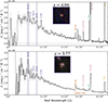 |
Fig. 1. NIRSpec/PRISM spectra of two N-emitters, illustrating the diversity of our sample. Top: Spectrum corresponding to a highly SF galaxy with strong optical lines. Bottom: Spectrum with a Balmer break at ∼3740 Å, a very low EW(Hβ), and faint optical lines. Both spectra show at least one significant UV nitrogen line. |
2.3. Extinction correction
We measured the colour excess, EB − V, from the Balmer decrement using the main Balmer lines from Hα to Hδ, adopting the extinction curve from Cardelli et al. (1989) and assuming standard nebular conditions (ne = 250 cm−3 and Te = 104 K). Owing to the limited PRISM resolution, the Hα and Hγ lines are blended with emission from [N II] λλ6550,6585 and [O III] λ4363, respectively. We therefore assume that the contribution from these neighbouring lines amounts to roughly ≃10% of the observed fluxes.
We calculated all available Balmer line ratios and compared them with the predicted values for a given EB − V and the adopted extinction curve. Our fiducial EB − V values are those that minimize χ2. For 20 sources, we find non-physical Balmer decrements, i.e. consistent with negative EB − V, although the uncertainties for several are consistent with positive reddening. For these cases, we adopt EB − V = 0. Sources with physical EB − V values exhibit a wide range of colour excesses, from ≃0.03 mag up to ≃2.7 mag, with LRDs being the most obscured. Finally, the spectra of nine sources show no or only one significantly detected Balmer line, and we conservatively assume EB − V = 0 for these objects. The full sample has a mean extinction of  and a median value close to zero. Finally, the rest-UV and optical emission line fluxes were corrected for extinction, adopting the Reddy et al. (2016) curve.
2.4. Literature samples
Our selection recovers several (four) previously known N-emitters reported in the literature: GN-z11, CEERS-1019, GN-z9p4, and UNCOVER-45924 (see Bunker et al. 2023; Marques-Chaves et al. 2024; Schaerer et al. 2024; Labbe et al. 2024). The recent compilation of Ji et al. (2026) includes 13 objects showing emission in N IV] λ1486 and N III] λ1750, which we define here as N-emitters2. Subsequently, three N-emitters were reported in the literature (MoM-z14, UNCOVER-3686, and CANUCS-LRD-z8.6 in Naidu et al. 2026; Fujimoto et al. 2024; Tang et al. 2026; Morishita et al. 2026). Two other lensed N-emitters, SMACS 2031 and the Lynx arc, at z ∼ 3.4 − 3.5 were discovered earlier (see Marques-Chaves et al. 2024; Patrício et al. 2016; Fosbury et al. 2003). Among these 18 N-emitters, 11 have MSA/PRISM observations, and four have been observed with medium- or high-resolution gratings. Our selection did not recover seven objects observed with MSA/PRISM – namely, GN-z8-LAE, GS-z9-0, GHZ9, GHZ2 = GLASS-z12, MoM-z14, UNCOVER-3686, and CANUCS-LRD-z8.6 – reported by Navarro-Carrera et al. (2025), Curti et al. (2025), Napolitano et al. (2025), Castellano et al. (2024), Naidu et al. (2026), Fujimoto et al. (2024), and Tripodi et al. (2025). In several of these, the detection of N lines is tentative, and our procedure and measurements do not yield significant (> 3σ) and robust detections for these objects. We therefore do not add them to our sample but subsequently compare our sample with that from the literature.
In short, combining the 18 previously known N-emitters with our sample of 42 new objects triples their number, bringing the total to 60 N-emitters to date. Note also that Martinez et al. (2025) report eight new objects at z ≲ 0.04 with N lines in the UV.
3. A new sample of N-emitters and candidates
3.1. Redshift, MUV, SFR, and stellar mass
The redshift and UV brightness distributions of the N-emitters are shown in the left panel of Fig. 2. The objects show a broad redshift distribution, from z = 14 to z ∼ 3, where the lower limit is determined by the minimum wavelength covered by the PRISM spectra (λmin ∼ 0.6 μm). Compared to the literature sample, our study adds many new objects at z ∼ 3 − 7. It also shows that N-emitters are found among fainter galaxies than previously known at least down to MUV ∼ −16.
 |
Fig. 2. Left: Absolute UV magnitude MUV of all known N-emitters (60 in total) vs. redshift. The literature sample is marked with crosses. The colours distinguish objects categorised as SFGs (blue), LRDs (black), and AGNs (red). The literature sample also includes four lensed galaxies, whose magnitudes have been corrected for gravitational lensing. Right: Mass–SFR showing a subset of the N-emitters (symbols colour-coded by redshift) with derived stellar masses, alongside the SF MS of Cole et al. (2025) at z = 7 − 9 (dashed line). |
We estimated stellar masses and star-formation rates (SFRs) for a subset of N-emitters with available JWST NIRCam photometry and NIRSpec prism spectra by performing spectral energy distribution (SED) fitting with Bagpipes (Carnall et al. 2018), adopting fixed spectroscopic redshifts. An up-to-second-order polynomial calibration was applied to correct residual slit-loss of the spectra compared to the photometry. We adopted a non-parametric star-formation history, BPASS stellar population models, the Salim et al. (2018) dust attenuation curve, and variable metallicities. Further methodological details will be presented elsewhere (Xiao et al., in prep.) We also derived the SFR from the dust-corrected Hα (or Hβ) line flux, following the relation from Kennicutt (1998). The resulting stellar mass–SFR relation is shown in the right panel of Fig. 2. Our sources broadly follow the main sequence (MS) of galaxies derived by Cole et al. (2025) in the redshift range 7 < z < 9. This choice of redshift range is somewhat arbitrary, as the MS does not significantly change with redshift. Interestingly, we find that the N-emitters cover a wide range of stellar masses (7.0 ≲ log(M★/M⊙)≲11.8). The highest-mass values should be treated with caution, as they correspond to LRDs, whose nature remains unclear. Excluding these objects, our sample spans a stellar mass range of 7.0 ≲ log(M★/M⊙)≲9.8, with a median value of log(M★/M⊙) = 9.13.
3.2. UV and optical emission lines of N-emitters
The broad wavelength coverage provided by the PRISM spectra enables the detection of multiple emission lines. In Table A.1 we report the rest-frame UV/optical emission lines detected in our sample, their occurrence rate (i.e. the number of detections in total), and the same information for the three N-emitter subcategories (SFG, LRD, and AGN). The rest-UV lines detected are N IV] λ1486, C IVλ1550, He IIλ1640, O III] λ1666, N III] λ1750, and C III] λ1909; we henceforth refer to these lines as N IV], C IV, He II, O III], N III], and C III] for simplicity. Although not included in our measurements, Lyα was detected in at least 12 sources.
By selection, all the 45 objects in our sample show N III] or N IV], and in ten objects we significantly detect both of these lines (see Fig. 3). A larger fraction (74%) of N-emitters show N IV], whereas ∼48% exhibit N III]. C III] or C IV lines are also detected, but only in a subset of our N-emitters. Finally, He II and/or O III] is detected in ∼24% of the objects, although the deblending of these lines is difficult. In the rest-optical domain, the majority of objects show forbidden [O II] λ3727 and [O III] λλ4959,5007 emission as well as H recombination lines, as expected (see Table A.1). For example, we detect both [O III] λλ4959,5007 and one or several H recombination lines in 40 objects. The remaining objects include two galaxies at z > 10, for which [O III] λλ4959,5007 falls outside the observed spectral range; objects with detected oxygen line but no H lines; and sources with low S/N in the optical. Finally, we note that the auroral line [O III] λ4363 is detected in two high-z sources, GN-z11 and a z = 7.256 source, which we classify as an LRD (Table B.1).
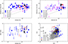 |
Fig. 3. Observed properties of N-emitters (SFG in blue, LRD in black, and AGN in red). The EWs of the UV lines (left: N III] λ1750, N IV] λ1486; right: C III] λ1909, C IVλ1550) are shown as a function of EW(Hβ) (top row). Typical error bars are comparable to symbol size and are therefore not shown. Upper limits for N IV] λ1486 and C IVλ1550 are indicated with blue arrows, while the limits for N III] λ1750 and C III] λ1909 are indicated with magenta arrows. The observed correlations of carbon-emitters from Tang et al. (2026) are shown as dotted and dashed lines (for C III] and C IV), for reference also in the top-left panel. Bottom: N IV] λ1486/N III] λ1750 vs. EW(Hβ) and O32 vs. R23. Symbols and colour codes are identical to the main plot. Bottom right: Low-z and high-z data from Izotov et al. (2021) and D’Eugenio et al. (2025). In all panels, 3σ limits are shown. The EWs are in the rest-frame. |
The strongest UV lines of our objects are generally N IV] or N III], although this is not a selection criterium. The C IV and C III] lines are either generally weak or altogether absent, but their EWs can reach comparable N line values. Typical EWs of N IV] and N III] are ∼10 − 50 Å. Similarly, for C IV and C III] the EWs range from ∼4 − 30 Å and are somewhat higher in objects classified as AGNs or LRDs (Fig. 3). In some objects, we detect nitrogen lines with lower EWs ≲10 Å; however, our measurements are limited by S/N and the strong wavelength dependence of the PRISM spectral resolution, a feature which nonetheless facilitates emission line detections with increasing redshift. In Fig. 3 we also compare our EW measurements to the typical EW values of C III] and C IV in SFGs, which are known to scale with the Hβ EW. We clearly see that, compared to typical SFGs at z ∼ 6 − 9 and at lower redshifts, the EW of the nitrogen lines can exceed those of C III] by a factor of up to ∼10. The same is also true for the C IV line.
Interestingly, the EWs of the optical lines (e.g. Hβ and [O III]λ5007, shown in Figs. 3 and C.2) of the N-emitters vary by more than one order of magnitude, ranging from the highest values typically observed (EW(5007) ∼2000 − 3000 Å) to as low as ∼100 Å (or EW(OIII+Hb) ≳130 Å). The mean EW(OIII+Hb) ≈1100 Å (for our z > 5 sources) is comparable to that reported by (Roberts-Borsani et al. 2024, ∼700 − 1000 Å) from stacks. Our results strongly contrast with those of Topping et al. (2025), who exclusively found N-emitters with very high EWs. See our discussion in Sect. 5.
The relative intensities of the UV nitrogen lines vary significantly, as shown in Fig. 3. Of course the dynamic range of the N43 = N IV] λ1486/N III] λ1750 ratio is somewhat limited, since these lines are relatively weaker (have lower EWs) than, for example, the optical [O III] and [O II] lines. We do not find a strong correlation between N43 and redshift (see Fig. C.1) or the optical line ratio O32 = [O III] λ5007/[O II] λ3727. However, N43 possibly increases on average for objects with stronger lines (higher EW(Hβ); see Fig. 3).
The carbon ionisation, traced by the C43 = C IVλ1550/C III] λ1909 ratio, behaves similarly to N43, although these lines are detected in fewer objects. In contrast, stacked UV spectra from large samples typically show C III] as the strongest emission line (after Lyα); consequently, C43 < 1, and N lines are either very weak or absent (cf. Roberts-Borsani et al. 2024; Hayes et al. 2025; Tang et al. 2026). This trend holds for high-z sources as well as for lower redshifts (z ∼ 2 − 5), as established by ground-based observations (Shapley et al. 2003; Le Fèvre et al. 2015).
The O32 ratio of our objects varies from ∼1 to 30 and correlates with the observed rest-optical emission line strengths (e.g. [O III] λ5007 and Hβ), as illustrated in Fig. C.2. The observed trend between O32 and EW([O III]) of the N-emitters follows that of SFGs at z ∼ 1 − 2 and up to z ∼ 9 from Tang et al. (2019, 2026) well. It could be somewhat steeper than the relation found by Izotov et al. (2021) from SDSS galaxies at z ∼ 0 − 1, also shown in this figure. The LRDs, where [O II] λ3727 is consistently undetected, stand out as extreme outliers in this figure.
The classical O32 versus R23 diagram (R23 = [O II] λ3727+[O III][O III] λλ4959,5007)/Hβ), which to first order traces ionisation and metallicity, is shown in Fig. 3 for the N-emitters and for other samples of SF galaxies from JADES DR3 (D’Eugenio et al. 2025) and Izotov et al. (2021). The N-emitters span a similar range as the objects from the JADES catalogue. Interestingly, we find N-emitters over a wide range of R23, including values up to the maximum observed, suggesting that these objects are not limited to very low metallicity, as previously reported.
4. Physical properties of N-emitters and candidates
4.1. Metallicities (O/H abundances) of N-emitters
We first determined the metallicities from the emission lines. Since auroral lines, such as [O III] λ4363 in particular, were only detected in two objects, we adopted the so-called strong line method using the recent calibrations of Sanders et al. (2025), which are based on the AURORA survey and a large compilation of JWST spectra. We primarily used [O II] λ3727, [O III] λλ4959,5007 and H lines (Hα, Hβ, or Hγ, depending on redshift), which can be used with the O2 = [O II] λ3727/Hβ, O3 = [O III] λλ4959,5007/Hβ, and  = 0.47 × log(O2) + 0.88 × log(O3) calibrations. We also used the new RO2Ne3 calibration, which involves the [Ne III] λ3869 line and is defined as RO2Ne3 = (NeIII+[O II] λ3727)/Hδ. We replaced the Hδ flux with Hβ or other stronger H lines, which are measurable with higher accurately, setting their relative fluxes to the standard case B values. Among these calibrations, two – O2 and RO2Ne3 – are monotic, i.e. single-valued, over the entire metallicity range covered by Sanders et al. (2025). To break the degeneracies of the remaining calibrations (O3 and
  ), we combined them with O2. We call these methods O3+O2 and
  +O2. Note also that we did not use the R23 calibration, since the high-z observations indicate that it is not sufficiently sensitive to O/H over a fairly broad range (see Sanders et al. 2025). We thus determined the metallicities for 28 objects with the O2 calibration, 15 with RO2Ne3, and 26 with O3+O2 and
  +O2. Finally, we adopted as our best estimate the mean 12 + log(O/H) values (up to 4). We did not use metallicities for objects classified as LRDs or AGNs, since the adopted calibrations are not appropriate for such objects.
As already suggested by the range of R23 ratios covered by our objects (Fig. 3), we find metallicities ranging from 12 + log(O/H)∼7.15 (∼3% solar) up to ∼8.5, or even close to solar, depending on the indicator used. A comparison of the metallicities derived with these calibrations and methods is shown in Fig. D.1 as a function of 12 + log(O/H) derived from the O2 calibration. Overall, the different metallicity indicators agree, albeit with significant large scatter. At the low- and high-metallicity end, the O2 and RO2Ne3 methods differ more strongly with differences of ∼0.3.
For seven additional objects with measurements only in O3 (i.e. with significant detections in both [O III]λ5007 and Hβ lines but not in [O II] λ3727), we find that the upper limits of O2 are compatible with the O/H estimate from the O3 calibration. We therefore adopted the O3 metallicities, which fall in the range 12 + log(O/H) = 7.15 − 7.93. We thus obtain 35 objects in total with estimated metallicities in the range 12 + log(O/H) = 7.15 − 8.5.
Given that our metallicity estimate includes the O2 calibration (when [O II] λ3727 is detected), we note that O/H may be underestimated, since [O II] λ3727 has a relatively low critical density (∼(1.3 − 4.8)×103 cm−3 for the two doublet lines) and could be affected (decreased) by collisions. However, the observed O32 ratios of most of our objects are not particularly high (see Fig. 3), indicating that this effect may be limited. Comparing our metallicity estimates for the three galaxies (GN-z11, GNz9p4, and CEERS1019) with literature values, we find that they agree within the quoted uncertainties, with the exception of GN-z11. For this object, we obtain 12 + log(O/H) = 7.54, which is ∼0.3 dex lower than previous literature values (Senchyna et al. 2024; Ji et al. 2026). From this and the differences illustrated in Fig. D.1, we estimate that our typical uncertainty on log(O/H) is ∼0.2 dex. Higher quality (S/N) and medium resolution spectra, which enable auroral line detections, are needed for more accurate abundance determinations.
4.2. CNO abundances of N-emitters
To derive and analyse the CNO abundances of our sample, we adopted several methods. First, we only used UV emission lines to determine (when possible) the relative abundances of C, N, and O, as they largely avoid corrections for attenuation and provide results that depend only very little on the (unknown and/or assumed) electron temperature and density.
We determined the following ionic abundance ratios:
![Mathematical equation: $$ \begin{aligned} 1.\ \frac{\mathrm{N}}{\mathrm{O}}(\mathrm UV)&\approx \frac{\mathrm{N^{+2}}}{\mathrm{O^{+2}}} \times \mathrm{ICF}=\frac{\mathrm{N^{+2}}}{\mathrm{O^{+2}}} \left[\frac{X(\mathrm N^{+2})}{X(\mathrm O^{+2})}\right]^{-1} , \end{aligned} $$](/articles/aa/full_html/2026/06/aa58256-25/aa58256-25-eq6.gif) (1)
(1)
![Mathematical equation: $$ \begin{aligned} 2.\ \frac{\mathrm{N}}{\mathrm{O}}(\mathrm UV)&\approx \frac{\mathrm{N^{+3}}}{\mathrm{O^{+2}}} \times \mathrm{ICF}=\frac{\mathrm{N^{+3}}}{\mathrm{O^{+2}}} \left[\frac{X(\mathrm N^{+3})}{X(\mathrm O^{+2})}\right]^{-1}, \end{aligned} $$](/articles/aa/full_html/2026/06/aa58256-25/aa58256-25-eq7.gif) (2)
(2)
 (3)
(3)
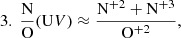
where X denotes the ionisation fraction. These ratios were derived from the N III], N IV], and O III] lines. The strength of O III] was inferred from the He IIλ1640+O III] λ1666 blend, assuming a typical ratio of He II/O III] = 0.25 following Tang et al. (2026). This is applicable to 11 N-emitters from our sample for which the He II+O III] blend is significantly detected. We then used the expressions of Villar-Martín et al. (2004) to determine the ionic abundance ratios and assume ionisation correction factors (ICFs) equal to 1. According to the recent calculations of Martinez et al. (2025) the above ICFs are all either > 1 or provide small corrections (≲20%) compared to our systematic uncertainties. Formally, our reported N/O values could therefore underestimate the true values.
We proceeded in the same way to determine up to three estimates of the C/O(UV) abundance ratio, using the C III] and C IV lines instead of the nitrogen lines. Moreover, we computed the N/C ionic abundance ratios (or lower limits thereof) using only the relative line intensities of the UV lines (see Appendix D). The main advantage of relative CNO abundances derived from UV lines is that they depend only weakly on the (unknown) electron temperature and are essentially independent of density (as long as ne ≲ 109 cm−3), as described further in Appendix D.
Finally, we derived N/O from the combination of UV and optical lines, obtaining the ionic N+2/H+ and N+3/H+ abundances (following Villar-Martín et al. 2004). We then calculated N/O(UV-opt) as
 (4)
(4)
where O/H is the metallicity derived previously (Sect. 4.1). When a single N line was detected, we simply adopted the corresponding ionic abundance ratio (i.e. (N+i/H+)/(O/H), where i = 2 or 3 and ICF = 1), without correcting for unseen ionisation stages of N. When lacking Te measurements for our objects, we adopted two cases to explore the importance of this effect. First, we adopted a variable Te = Te([O III]), empirically derived from galaxy samples with [O III] λ4363 auroral line detections. These samples exhibit a well-known average relation between Te and metallicity (O/H), as shown, for example, in Fig. D.2 for the SDSS sample of Izotov et al. (2021) and the JWST AURORA survey at z ∼ 2 − 3 from Sanders et al. (2025). We also adopted a minimum temperature of Te = 15 000 K, as well as a constant value of Te = 22 000 K. This latter value is relatively high, especially for galaxies with metallicities 12 + log(O/H)≳8.0, and yields lower N/O values.
The relative N/O abundances of the N-emitters, derived for the two values of Te and using the different methods explained above, are shown in Fig. 4 as a function of the adopted metallicity. For comparison, we also show the measured abundances in the H II regions and SF galaxies at low-redshift along with the average evolution of N/O-O/H. Clearly, the N/O abundance ratios of the vast majority of our N-emitters are high compared to typical galaxies and are significantly super-solar3, regardless of their metallicity and the adopted electron temperature. For objects where the abundances can be derived from UV lines only, we find log(N/O(UV)) ∼ − 0.75 − 0 across the different methods, over a wide range of metallicities and largely independently of the assumed electron temperature. These N/O(UV) values are comparable to those found previously for the known N-emitters (see e.g. Ji et al. 2026).
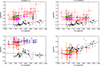 |
Fig. 4. CNO abundance ratios of the N-emitters (coloured symbols) as a function of metallicity (O/H). Top left: N/O abundances computed using variable Te(O/H); top right: for fixed Te = 22 000 K. The coloured squares show the N/O(UV) values from UV lines only (orange, magenta, and green for Eqs. (1), (2), and (3)). The red diamonds show N/O(UV-opt) derived from UV and optical lines following Eq. (4). Bottom left: N/C and lower limits from UV lines (blue); bottom right: C/O, using same coloured symbols. Low-z SF galaxies and H II regions from the compilation of Izotov et al. (2023) are shown as small black symbols. The dash-dotted lines show the average trends observed in low-z SF galaxies, as parametrised by Vila-Costas & Edmunds (1993) and Nicholls et al. (2017). |
Interestingly, several N-emitters reported in Fig. 4 exhibit log(N/O) > 0, surpassing values previously reported for an LRD (UNCOVER-45924) and an AGN (GS-3073 in the high-density region), which has abundance ratios of log(N/O)  and log(N/O)
  , respectively (Ji et al. 2026). Indeed, using the method combining the UV and optical lines, we find several objects with N/O(UV-opt) exceeding the solar N/O value by factors of ≳30 (1.5 dex), i.e. log(N/O) ≳0.6. The trend of increasing N/O with O/H obtained with this method (left panel of Fig. 4) is driven by our coupling of the electron temperature to O/H (variable Te). In contrast, the right panel shows the results for a constant Te = 22 000 K in the line-emitting region, yielding relatively constant N/O values across O/H and less extreme, yet still super-solar, values for the majority of objects.
The relative N/C and C/O abundances of our N-emitters and the low-z comparison samples are also shown in Fig. 4. Regardless of the method used, we find high N/C values (typically log(N/C) ∼0.3 − 1), comparable to or somewhat higher than earlier findings (cf. Marques-Chaves et al. 2024; Ji et al. 2026; Isobe et al. 2025). The lower limits, derived from UV line ratios when neither C III] λ1909 nor C IVλ1550 is detected, also consistently show that nitrogen is strongly enhanced with respect to carbon in all N-emitters. The C/O ratios of the majority of objects are comparable to those of typical metal-poor SF galaxies, although there are hints of somewhat lower C/O values in some objects. The C/O ratios found in our new N-emitters span a similar range to those found earlier (see e.g. Marques-Chaves et al. 2024; Ji et al. 2026). It is difficult to derive accurate limits on C/O, i.e. using the UV ratio of C III]/O III], since few objects exhibit O III] (or He II+ O III]) detections.
To summarise, we find that the majority, if not all N-emitters, show super-solar N/O abundances and a significant enhancement in N/O and N/C compared to typical galaxies with the same metallicity (O/H). When two or more UV emission lines of C, N, or O are detected, we can determine relatively accurate abundance ratios for these elements, for three reasons. 1) Their emissivities depend in a similar fashion on the (unknown) electron temperature. 2) The critical density of the emission lines is very high (e.g. > 109 cm−3 for N III] and O III] which yield the ionic ratio N+2/O+2, and ∼105 − 109 cm−3 for C III]). 3) The ionisation correction is quite small (< 0.2 − 0.3 dex), in particular for N+2/O+2 and N+2/C+2 (Martinez et al. 2025). Consequently, we find consistently high N/O and N/C ratios, along with high lower limits on the latter, across a wide range of metallicities (O/H), from a few percent of solar up to nearly solar. Since our metallicities are derived only using strong line methods, we consider these to be fairly uncertain. Better observations, allowing one to determine electron temperature and density, ideally from multiple tracers, are required to obtain more accurate metallicities.
4.3. Morphologies of N-emitters
We retrieved automatic morphological parameters from DJA, which were derived using SourceXtractor++ by fitting Sersic models to JWST NIRCam images4. Effective radii are available for 28 of 45 N-emitters. They range from the unresolved detection limit (Reff ≲ 90 pc) up to Reff ≈ 2.7 kpc. We also examined their stellar mass and SFR surface densities, derived from these morphological parameters for a subset of the N-emitters (see Appendix C.2) Visual inspection of the NIRCam images further reveals that these objects do not necessarily appear compact. We find a surprising diversity of morphologies among the N-emitters in our sample. In addition to compact sources, similar to those reported in previous studies such as GN-z11 (Álvarez-Márquez et al. 2025), GHZ2 (Calabrò et al. 2024) and GN-z9p4 (Schaerer et al. 2024), we also identify clumpy objects and possible spiral structures at z ∼ 3.5. (see Fig. 5). For comparison, CEERS-1019 (Marques-Chaves et al. 2024) likewise contains three different compact clumps. Many of the objects in our sample exhibit extended shapes. We show four representative examples of these N-emitters in Fig. 5.
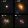 |
Fig. 5. NIRCam F115W, F356W, and F444W composite 1″ × 1″ images of four N-emitters from our sample, highlighting the morphological diversity within the population, including compact, disky, and clumpy structures. |
We do not observe any clear trend of morphological evolution with redshift. This result contrasts with findings from earlier studies (Schaerer et al. 2024; Harikane et al. 2025; Topping et al. 2025), which reported that high-redshift N-enhanced galaxies are significantly more compact than typical SF galaxies, suggesting that both star formation and stellar mass are strongly concentrated in dense regions. Thus, the N-emission could come from one of the clumps within these objects.
5. Discussion
5.1. Diversity among N-emitters
In contrast to earlier findings, one of the salient results of our study is that N-emitters show a wide diversity of multiple properties. For example, N-emitters are found across a wide range of stellar masses, SFR (Sect. 3.1) and metallicities (Sect. 4.1), in both very compact objects and spatially resolved galaxies with diverse morphologies (Sect. 4.3), and exhibiting a broad variety of optical emission line strengths (Sect. 3.2). Previously, N-emitters identified with JWST were known to be limited to objects with relatively high UV brightness (MUV ≲ −19.5), low metallicity (12 + log(O/H)≲8.0), compact (or unresolved) size, and very high EWs in [O III] λ5007 and/or Hβ (see e.g. Marques-Chaves et al. 2024; Schaerer et al. 2024; Harikane et al. 2025; Ji et al. 2026; Topping et al. 2025). We now discuss how these findings can be reconciled and what these results tell us about the phenomenon and nature of N-emitters.
As shown in Sect. 3.2, our sample of N-emitters spans a wide range of EW(Hβ) values. These peculiar objects are not only found at the highest EWs, as previously reported for known N-emitters, but also extend down to ∼10 Å in the most extreme case, where Hβ is often very faint or barely detected. Interestingly, most of these low-EW sources appear spatially extended, except for two objects that are either quite compact but faint (MUV ≳ −17) or display noisy spectra. Moreover, we identify clear Balmer breaks in several spectra, suggesting the presence of older stellar populations (see Fig. 1). We examined all galaxies showing a Balmer break and find that they also exhibit low EW(Hβ) values (up to 50 Å), indicating that N-emitters are not necessarily dominated by very young or recently formed stellar populations.
The fact that the majority of low-EW(Hβ) sources are extended and show colour variations suggests that they contain a mixture of stellar populations of different ages. In this case the (small, ∼0.2″) region sampled by the JWST MSA spectrum could contain both a young SF region producing the bulk of the UV emission and the emission lines, and an older population (≳50 − 100 Myr) that is revealed by the Balmer break and effectively ‘dilutes’ (reduces) the EWs of the optical emission lines. Nitrogen lines in the UV with similar EWs, independently of EW(Hβ) (Fig. 3), also supports the presence of a young stellar population in all the objects. Our observations, therefore, indicate that strong N-emitting regions are likely relatively young (≲10 Myr), although their exact age cannot be inferred from our data.
Similarly, the spatial extension of many of our objects does not contradict earlier findings that N-emitters are essentially found in systems with very high stellar mass and SFR surface densities, as well as in very compact objects. The two observations can be reconciled if nitrogen emission originates from a small, localised region in the galaxy probed by the JWST aperture, which would reveal these ‘extreme’ conditions. Future observations – for example, with integral field spectroscopy – can, in principle, verify this hypothesis by measuring the spatial extension of the N-emission and N/O enrichment, testing whether the interstellar medium (ISM) densities in these regions are as high as the densities found in earlier N-emitters, among others.
Finally, our discovery of N-emitters across a wider range of metallicities and UV brightnesses than in previous studies is consistent with those results. We attribute this to our systematic search of a large number of spectra (i.e. yielding increased statistics; see below) and the extension of our search to lower redshifts, where both higher-metallicity and UV-fainter galaxies are accessible.
5.2. Statistical estimates of the N-emitter population
To compare the known and newly identified N-emitters with the total galaxy population and provide a first estimate of their relative fraction, we used DJA to identify emission lines galaxies (ELGs). We searched for one or multiple emission lines with a significance ≥4σ in the rest-UV and rest-optical domains among all NIRSpec PRISM spectra with reliable redshifts (grade = 3)5. We also counted galaxies with no detectable emission lines and accounted for multiple entries of the same object in the database. The total sample includes 8323 unique sources above z ≥ 3. The result is shown in Fig. 6.
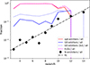 |
Fig. 6. Redshift evolution of the fraction of N-emitters (black diamonds), combining the literature and our sample, among all available NIRSpec PRISM spectra with robust redshifts (grade = 3) from the DJA dataset. The blue lines show the fraction of the rest-UV line emitters 4σ (solid) or 3σ detection (dotted) thresholds, respectively. The red line indicates the fraction of objects with rest-optical emission lines, while the magenta lines indicates all ELGs (UV and/or optical). At z ≳ 11 the number of objects is very small (< 10 per bin), and few objects show emission lines. |
We find that the fraction of N-emitters, fN, increases strongly with redshift, when compared to all galaxies, galaxies with emission lines, and objects with UV emission lines only (‘UV emitters’ in short). This trend is well described by
 (5)
(5)
The fraction ranges from ≲1% of all galaxies with PRISM spectra at z ≲ 6 to more than 10% at z ≳ 10. Since galaxies with emission lines dominate the total number of entries in DJA (by at least over 3 ≲ z ≲ 10), these values are also similar to those of N-emitters among emission line galaxies. Compared to galaxies showing UV emission lines, N-emitters represent ∼5 − 10% at z ∼ 3 − 6, depending on the adopted threshold (3 or 4σ) for the automatic detection of UV lines. At z ≳ 10 the fraction of N-emitters appears to be very elevated (up to ∼30%), although the statistics are low at these redshifts. At z ≳ 9 the detection of rest-optical emission lines becomes more difficult, since the strongest lines ([O III] λ5007, in most cases) are excluded from the spectral range covered by NIRSpec. This explains the decrease in this population in Fig. 6. Since the DJA data used here come from a variety of programs with different selection criteria and depths, it is difficult to interpret precisely the fractions derived here. However, since both N-emitters and ‘UV-emitters’ rely on the detection of UV lines and thus have similar detectability, their relative fraction should be well determined and meaningful. And clearly, the fraction of N-emitters among ‘UV emitters’ increases by a factor of ∼6 or more between z ∼ 3 and 12.
The fact that N-emitters are rare, at least over redshifts z ∼ 3 − 10 is not new; nevertheless, they are quantified here for the first time. Indeed, large and deep ground-based spectroscopic surveys undertaken with Keck and VLT have provided detailed rest-UV spectra for large numbers of galaxies from z ∼ 2 − 6, showing no detection of N IV] λ1486 or N III] λ1750 in stacks (e.g. Shapley+, Du+2018, Lefevre+2019, and Carilli+2021) and revealing very few peculiar objects with these features (Vanzella et al. 2010; Übler et al. 2023, e.g. GS-3073 at z = 5.55, a N-emitter confirmed as AGN with JWST). Similarly, stacks of JWST spectra show either no or weak emission N III] or N IV] emission lines at z ∼ 4 − 9, indicating that N-emitters are a rare population at these redshifts (Roberts-Borsani et al. 2024; Hayes et al. 2025). Finally, stacking the spectra of ten galaxies at z > 10, Roberts-Borsani et al. (2025) detected N IV] λ1486 in a subset of galaxies exhibiting C IVλ1550 emission, thereby also inferring high N/O and N/C abundance ratios. These findings are fully consistent with our results, which show a strong increase in the N-emitter fraction with redshift and a transition from rare to fairly common objects at z > 10.
5.3. On the nature of N-emitters
As mentioned in the introduction, different scenarios have been proposed to explain the nitrogen enhancement observed in GN-z11 and the observed abundances in the more recently discovered N-emitters. Since our work significantly expands the ‘parameter space’ over which N-emitters are found and provides a first statistical estimate of the N-emitter population, we examine how this could constrain their nature or test these scenarios.
5.3.1. Constraints from metallicity and relative N/C abundances
So far N-emitters were only known at low-metallicity, with only one or two objects above 12 + log(O/H)≳8.0 in the compilation of Ji et al. (2026). If N-emitters also exist at higher metallicity, as our work suggests, metallicity-independent scenarios must be invoked. Furthermore, our finding of high N/C abundance ratios and lower limits (log(N/C) ≳ 0.5 for the bulk of N-emitters) strongly constrains these scenarios. Our data indicate abundance ratios typical of ejecta from H-burning and show no significant carbon contribution, i.e. He-burning products, expected to be ejected in copious amounts by WR populations that include WC and/or WO stars.
For example, the models of Kobayashi & Ferrara (2024) and Bekki & Tsujimoto (2023) for GN-z11 predict both an increase in N/O and C/O, yielding N/C values close to solar when the observed N/O value is reached. Our N-emitter data are incompatible with this prediction. In other models tracking the ejecta of normal stellar populations, a high N/O is reached at ∼3 Myr at low metallicities; C/O increases shortly thereafter (e.g. Charbonnel et al. 2023; Marques-Chaves et al. 2024; Shi et al. 2026). To reproduce our high N/C values without resulting in high C/O ratios, very young ages (∼3 − 4 Myr only) or the absence of WC stars must be invoked (Marques-Chaves et al. 2024; Tapia et al. 2024; Shi et al. 2026). For the Sunburst star cluster case, for example, this might be a valid explanation (see Pascale et al. 2023; Welch et al. 2025), but for a relatively large sample this is not plausible. Furthermore, since the ejecta of WR stars and the relative contribution of WC stars increase with metallicity in normal stellar populations (e.g. Mollá & Terlevich 2012), N-enriched objects should become progressively more C-enriched at higher increasing metallicities, contradicting our finding of consistently high N/C and N/O ratios regardless of metallicity.
5.3.2. Constraints from the statistics of N-emitters
Our quantification of the N-emitter fraction and its evolution with redshift (Fig. 6) could provide new insights into their nature and the sources of N-enhancement. We only briefly outline some ideas here and defer a more detailed analysis to future work.
Scenarios attributing N-enhancement to WR star ejecta would predict stronger and more sustained enhancements at lower redshifts. This is because the population of WR stars increases with metallicity, which generally increases on average over cosmic time. This would therefore lead to a redshift trend opposite to the one observed. However, if N-emitters correspond to a brief, young phase, as suggested by the Globular Cluster (GC) scenario, pollution from massive stars (WR, VMS, or SMS), and the detection of very high Hβ EWs (Topping et al. 2025, and our work), the increase in fN with redshift could be explained by increasing burstiness with z. This trend is supported by numerous observations and simulations (e.g. Cole et al. 2025). If this effect dominates over the metallicity dependence discussed previously, it could also reconcile the WR scenario with observations. Alternatively, the formation of WR stars might also be enhanced at high-z, for example, due to rapid stellar rotation or stellar initial mass functions (IMFs) favouring massive stars (Choi et al. 2017; Hutter et al. 2025).
On the other hand, if N originates mainly from older stellar populations, such as AGB stars, as proposed by D’Antona et al. (2023, 2025), McClymont et al. (2025), then N-enhancements would be expected in objects with lower EW(Hβ), as demonstrated in the simulations of McClymont et al. (2025). If burstiness increases and the typical burst duration of galaxies decreases with redshift (e.g. Ciesla et al. 2024; Cole et al. 2025), we would expect such a scenario to predict a decreasing fraction fN towards high-z. It remains, however, to be examined in detail whether this holds up and if it can be used as a test of the AGB and differential outflow models.
There are several ways to explain the observed increase in fN with redshift, including 1) an IMF evolution, leading to a flatter IMF or a higher upper mass limit of the IMF, thus increasing the yields of massive stars (WR or VMS; e.g. Higgins et al. 2025); and 2) an evolution of other conditions leading to enhanced N production in compact high-density regions, such as the formation of SMSs in the core of very compact star clusters (see Gieles et al. 2018, 2025). The latter, or perhaps both, offers a natural explanation, supported by the following observations: a shift towards higher SFR surface densities, ΣSFR, (on average) with increasing z (e.g. Morishita et al. 2024); the correlation between ΣSFR and gas pressure in galaxy disks (e.g. Krumholz et al. 2012); the increase in the average electron density with redshift (e.g. Isobe et al. 2023; Martinez et al. 2025); and the concommitant increase in the cluster formation efficiency (CFE), which favours the formation of massive gravitationally bound systems, such as proto-GCs (Kruijssen 2026). Last, but not least, this picture is also supported by the similarity between the observed abundance ratios in N-emitters and GCs (Charbonnel et al. 2023; Senchyna et al. 2024) as well as the high formation redshifts of GCs. If star-formation in these very dense clusters leads to WR, VMS, or even SMS, and enables or facilitates the retention of the enriched material within the cluster (see simulations of Shi et al. 2026), it would naturally produce localised N-enriched regions with increasing frequency at high-z. This is our favoured scenario, which could potentially work with different nucleosynthetic sources (WR, VMS, and SMS), which remain to be identified.
5.3.3. Other properties and constraints
While the majority of N-emitters reported so far in the literature are very bright (MUV ∼ −22 to −19.5, see Fig. 2), the strongly lensed Sunburst cluster is considerably fainter (MUV ≈ −18.6, adopting a magnification factor of ∼70). Our sample confirms that N-emitters are found over a wide range of absolute scales, which include fainter objects (MUV down to −17 or fainter) in particular. Also, the host galaxies of our sample are found over a wide range of stellar masses and SFRs, indicating that N-emitters are not limited to a specific mass or luminosity range.
As already discussed in Sect. 5.1, our observations a priori relax the age constraints on N-emitters, since they show a wide range of Hβ EWs, in contrast to earlier, smaller samples that suggested N-emitters are associated only with very young ages (Topping et al. 2025). However, our observations also show signs of composite stellar populations, which complicate age determinations and do not exclude nitrogen emission from a young region. Spatially resolved follow-up observations will be crucial for answering this question and deriving useful ages to constrain nitrogen source(s).
Finally, we would like to comment on the fact that ∼13% (six out of 45) N-emitters of our sample are LRDs, and several LRDs were already known to show nitrogen UV emission lines (e.g. UNCOVER-45924 and CANUCS-LRD-z8.6, Ji et al. 2026; Morishita et al. 2026). This, together with the finding that other properties – such as compactness and unusually high-density gas – are found in (at least some) N-emitters and LRDs, indicates that these objects share relatively unusual physical properties. While the nature of the N lines and nucleosynthetic sources hosted in ‘star-forming’ N-emitters and LRDs remain unknown, one could speculate that the N-enrichment observed in both has the same origin. If this is true and LRDs host massive black holes, as generally postulated, it would suggest that some SF N-emitters contain SMSs, which could produce the observed ejecta and abundance ratios and subsequently collapse into intermediate-mass black holes (see Charbonnel et al. 2023; Marques-Chaves et al. 2024), thereby forming the seeds for black holes in LRDs. Future studies exploring possible links between these two puzzling classes could shed more light on their nature.
5.4. Caveats and open questions
Finally, we briefly discuss some of the main caveats of our work, open questions, and possible future directions. The physical interpretation of our results is subject to several uncertainties, primarily related to the derivation of chemical abundances and the limitations of the current dataset. First, the abundance estimates rely on dust-corrected fluxes and, as discussed in Sect. 2.3, several sources in our sample exhibit negligible or even non-physical EB − V values possibly due to the limited spectral resolution of the PRISM data. This suggests that, on average, the derived EB − V values may be underestimated. Nevertheless, this possible limitation does not affect our main conclusion. For higher extinction levels, the dust-corrected fluxes of the UV nitrogen lines (N IV] and N III]) increase more strongly than the optical oxygen lines used to compute N/O. As such, adopting higher extinction corrections would further increase the inferred N/O ratios. However, this does not affect the N/O ratios determined exclusively from UV lines.
A further source of uncertainty arises from the lack of direct Te measurements. The [O III] λ4363 auroral line was detected in only one source, which prevented us from determining Te for the bulk of the sample. As a result, O/H was derived using strong-line calibrations (Sect. 4.1), which are uncertain and could introduce systematic offsets. In addition, the electron densities of the N-emitting regions remain unconstrained due to the PRISM resolution, and thus, we cannot directly assess the presence of density gradients. Nevertheless, the detection of lines with relatively low critical densities in the majority of sources (e.g. [O II] λ3727, see Table A.1) suggests that strong collisional de-excitation is unlikely to dominate the observed line ratios. Therefore, strong line methods should provide a reasonable estimate of the metallicity (O/H) of N-emitters, at least on average. Furthermore, N/C and N/O ratios determined from UV lines are not very sensitive to the electron temperature and density and should thus be relatively robust (see Appendix D). More accurate abundance determinations accounting for the likely presence of density and temperature gradients in N-emitters – as for example, shown by the detailed studies of (Martinez et al. 2025; Berg et al. 2025) – will require observations with higher S/N and spectral resolution.
To better characterise the physical properties of N-emitters, test different scenarios, and thus ultimately understand the nature of N-emitters, we will need to spatially resolve these objects and map fundamental properties such as relative abundances, ISM properties (density and temperature), stellar populations, and ideally ionised gas kinematics. This is, in principle, feasible – for example, using JWST NIRSpec IFU or with ELTs – for strongly lensed objects, and our study has identified additional objects that allow spatially resolved studies.
6. Conclusions
We carried out a systematic search for N-emitters, objects showing emission in one of the N III] λ1750 and N IV] λ1486 emission lines in the UV, using more than 20 000 JWST NIRSpec low-resolution (PRISM) spectra of ∼8300 unique sources at z > 3 available in the DAWN JWST Archive. Following an automatic preselection, tailored measurements, and careful inspection of the 2D and 1D spectra, we identified 45 robust N-emitters between redshifts z ∼ 3 − 11, including four previously known objects (GN-z11, CEERS-1019, GN-z9p4, and UNCOVER-45924). Our study effectively triples the number of known N-emitters.
Using the available spectra, multi-band images and photometric catalogues, we then analysed the global properties of the N-emitters (morphology, stellar mass, SFR etc.), characterised the observed spectroscopic properties (e.g. line strengths and excitation), estimated their metallicities (O/H abundance ratio), and determined the chemical abundance ratios of C, N, and O in these objects. Finally, we also determined, for the first time, a statistical measure of the population of N-emitters and its evolution with redshift.
Our main results can be summarised as follows:
-
N-emitters are found among a wide range of galaxies, in terms of morphology, UV magnitude, stellar mass, SFR, and metallicity. Morphologies range from very compact or unresolved objects, as previously identified, to extended galaxies showing multiple clumps, spatial colour variations, among others. Stellar masses range from ∼107 to 6 × 10⁹ M⊙, SFR ∼1 − 100 M⊙ yr−1, and absolute UV magnitudes vary between MUV ∼ −16 and −22 (Fig. 2).
-
Among the 45 N-emitters, we classified six objects as LRDs, based on compactness, SED shape, and the presence of broad H lines, and four as broad-line AGNs.
-
The UV nitrogen lines show typical EWs between ∼5 Å and up to ∼100 Å in a few cases. Diverse ionisation conditions, as traced by N IV] λ1486/N III] λ1750 are observed. Carbon lines (C IVλ1550 and C III] λ1909) are generally fainter than the N lines (Fig. 3).
-
The rest-optical emission lines of N-emitters show a wide range of ionisation and metallicities, as traced by O32 and the relative intensities of [O II] λ3727, [O III] λλ4959,5007, and Hβ (R23, see Fig. 3). Using different strong-line calibrations established at high-redshift, we find metallicities from 12 + log(O/H)∼7.15 − 8.5, extending the metallicity range of z > 3 N-emitters to metallicities above ≳20% solar (12 + log(O/H)≳8.0) compared to earlier studies.
-
The Hβ EW of N-emitters also varies strongly from EW(Hβ) ∼300 Å to 10 Å, and sources with low EWs show clear signs of a Balmer break, indicative of composite stellar populations combining both young (≲10 Myr) stars responsible for the emission lines and an older population (≳50 − 100 Myr) contributing significantly to the rest-optical spectrum.
-
The relative abundances of N, C, and O show clear signs of high N/O (super-solar values, log(N/O) ∼ −0.7 to 0 or higher) in all N-emitters. If the electron temperature in N-emitting regions decreases with increasing metallicity, the inferred N/O ratios could even increase with O/H. C/O abundances are ‘normal’ compared to those in galaxies at the same metallicity (O/H). Interestingly, all N-emitters show high N/C ratios and lower limits (log(N/C) ≳ 0.5), regardless of metallicity. The observed abundance ratios are compatible with ejecta from H-burning (CNO equilibrium) and do not show signs of carbon enhancements, even at higher metallicities (Fig. 4).
-
Comparing the N-emitter population with all ELGs, we find a significant increase in the fraction of N-emitters with redshift, ranging from few times 10−3 at z ≈ 3 to 10 − 30% at very high-redshifts (z ≳ 10). We suggest that this can be naturally explained if N-enhancement traces young, compact star clusters (possibly with IMFs favouring high-mass stars), whose frequency increases with redshift (Sect. 5.3).
Overall, our study has increased the sample of known N-emitters by a factor of ∼3 and shows that their parameter space is larger than previously thought: the phenomenon of strong UV N emission is not restricted to very compact objects, very low metallicities, or objects with very strong emission lines (e.g. high EW(Hβ)), as suggested in earlier studies (Marques-Chaves et al. 2024; Schaerer et al. 2024; Harikane et al. 2025; Topping et al. 2025). Despite this diversity, all N-emitters show enhanced N abundances (e.g. high N/O) – likely reflecting the initial selection (cf. Zhu et al. 2025) – and, interestingly, also show high N/C abundance ratios or lower limits. These results, together with our finding of an increased N-emitter fraction with redshift, now provide new and broader observational constraints on the nature of N-emitters. We compared existing scenarios with this data, showing, for example, that the overall absence of C enhancement places stringent constraints on nucleosynthetic sources. We hope this will enable future detailed studies – including spatially resolved information – to identify the main sources and physical processes governing enigmatic N-emitters and to understand their importance in the global picture of galaxy formation and evolution.
References
- Álvarez-Márquez, J., Crespo Gómez, A., Colina, L., et al. 2025, A&A, 695, A250 [NASA ADS] [CrossRef] [EDP Sciences] [Google Scholar]
- Arellano-Córdova, K. Z., Méndez-Delgado, J. E., Flury, S. R., et al. 2026, MNRAS, 547, stag380 [Google Scholar]
- Asplund, M., Grevesse, N., Sauval, A. J., & Scott, P. 2009, ARA&A, 47, 481 [NASA ADS] [CrossRef] [Google Scholar]
- Bekki, K., & Tsujimoto, T. 2023, MNRAS, 526, L26 [NASA ADS] [CrossRef] [Google Scholar]
- Berg, D. A., Naidu, R. P., Chisholm, J., et al. 2025, ApJ, accepted [arXiv:2511.13591] [Google Scholar]
- Bhattacharya, S., & Kobayashi, C. 2026, MNRAS, 548, stag545 [Google Scholar]
- Brammer, G. 2023, https://doi.org/10.5281/zenodo.7299500 [Google Scholar]
- Bunker, A. J., Saxena, A., Cameron, A. J., et al. 2023, A&A, 677, A88 [NASA ADS] [CrossRef] [EDP Sciences] [Google Scholar]
- Calabrò, A., Castellano, M., Zavala, J. A., et al. 2024, ApJ, 975, 245 [CrossRef] [Google Scholar]
- Cameron, A. J., Katz, H., Rey, M. P., & Saxena, A. 2023, MNRAS, 523, 3516 [NASA ADS] [CrossRef] [Google Scholar]
- Cardelli, J. A., Clayton, G. C., & Mathis, J. S. 1989, ApJ, 345, 245 [Google Scholar]
- Carnall, A. C., McLure, R. J., Dunlop, J. S., & Davé, R. 2018, MNRAS, 480, 4379 [Google Scholar]
- Castellano, M., Napolitano, L., Fontana, A., et al. 2024, ApJ, 972, 143 [Google Scholar]
- Charbonnel, C., Schaerer, D., Prantzos, N., et al. 2023, A&A, 673, L7 [NASA ADS] [CrossRef] [EDP Sciences] [Google Scholar]
- Choi, J., Conroy, C., & Byler, N. 2017, ApJ, 838, 159 [NASA ADS] [CrossRef] [Google Scholar]
- Ciesla, L., Elbaz, D., Ilbert, O., et al. 2024, A&A, 686, A128 [NASA ADS] [CrossRef] [EDP Sciences] [Google Scholar]
- Cole, J. W., Papovich, C., Finkelstein, S. L., et al. 2025, ApJ, 979, 193 [Google Scholar]
- Curti, M., Witstok, J., Jakobsen, P., et al. 2025, A&A, 697, A89 [Google Scholar]
- D’Antona, F., Vesperini, E., Calura, F., et al. 2023, A&A, 680, L19 [NASA ADS] [CrossRef] [EDP Sciences] [Google Scholar]
- D’Antona, F., Ventura, P., Marino, A. F., et al. 2025, A&A, 700, A265 [NASA ADS] [CrossRef] [EDP Sciences] [Google Scholar]
- D’Eugenio, F., Cameron, A. J., Scholtz, J., et al. 2025, ApJS, 277, 4 [Google Scholar]
- Fernández, V., Amorín, R., Firpo, V., & Morisset, C. 2024, A&A, 688, A69 [NASA ADS] [CrossRef] [EDP Sciences] [Google Scholar]
- Fosbury, R. A. E., Villar-Martín, M., Humphrey, A., et al. 2003, ApJ, 596, 797 [NASA ADS] [CrossRef] [Google Scholar]
- Fujimoto, S., Wang, B., Weaver, J. R., et al. 2024, ApJ, 977, 250 [NASA ADS] [CrossRef] [Google Scholar]
- Gieles, M., Charbonnel, C., Krause, M. G. H., et al. 2018, MNRAS, 478, 2461 [Google Scholar]
- Gieles, M., Padoan, P., Charbonnel, C., Vink, J. S., & Ramírez-Galeano, L. 2025, MNRAS, 544, 483 [Google Scholar]
- Harikane, Y., Inoue, A. K., Ellis, R. S., et al. 2025, ApJ, 980, 138 [NASA ADS] [Google Scholar]
- Hayes, M. J., Saldana-Lopez, A., Citro, A., et al. 2025, ApJ, 982, 14 [Google Scholar]
- Heintz, K. E., Brammer, G. B., Watson, D., et al. 2025, A&A, 693, A60 [Google Scholar]
- Henry, R. B. C., Edmunds, M. G., & Köppen, J. 2000, ApJ, 541, 660 [NASA ADS] [CrossRef] [Google Scholar]
- Higgins, E. R., Vink, J. S., Hirschi, R., Laird, A. M., & Sabhahit, G. 2025, A&A, 699, A71 [NASA ADS] [CrossRef] [EDP Sciences] [Google Scholar]
- Hutter, A., Cueto, E. R., Dayal, P., et al. 2025, A&A, 694, A254 [NASA ADS] [CrossRef] [EDP Sciences] [Google Scholar]
- Isobe, Y., Ouchi, M., Nakajima, K., et al. 2023, ApJ, 956, 139 [NASA ADS] [CrossRef] [Google Scholar]
- Isobe, Y., Maiolino, R., D’Eugenio, F., et al. 2025, MNRAS, 541, L71 [Google Scholar]
- Izotov, Y. I., Guseva, N. G., Fricke, K. J., et al. 2021, A&A, 646, A138 [NASA ADS] [CrossRef] [EDP Sciences] [Google Scholar]
- Izotov, Y. I., Schaerer, D., Worseck, G., et al. 2023, MNRAS, 522, 1228 [NASA ADS] [CrossRef] [Google Scholar]
- Ji, X., Übler, H., Maiolino, R., et al. 2024, MNRAS, 535, 881 [NASA ADS] [CrossRef] [Google Scholar]
- Ji, X., Belokurov, V., Maiolino, R., et al. 2026, MNRAS, 545, staf2110 [Google Scholar]
- Kennicutt, R. C., Jr. 1998, ApJ, 498, 541 [Google Scholar]
- Kobayashi, C. 2026, in Encyclopedia of Astrophysics, Volume 2, 744 [Google Scholar]
- Kobayashi, C., & Ferrara, A. 2024, ApJ, 962, L6 [NASA ADS] [CrossRef] [Google Scholar]
- Kruijssen, J. M. D. 2026, in Encyclopedia of Astrophysics, Volume 4, 500 [Google Scholar]
- Krumholz, M. R., Dekel, A., & McKee, C. F. 2012, ApJ, 745, 69 [Google Scholar]
- Labbe, I., Greene, J. E., Matthee, J., et al. 2024, ApJ, submitted [arXiv:2412.04557] [Google Scholar]
- Le Fèvre, O., Tasca, L. A. M., Cassata, P., et al. 2015, A&A, 576, A79 [Google Scholar]
- Luridiana, V., Morisset, C., & Shaw, R. A. 2015, A&A, 573, A42 [NASA ADS] [CrossRef] [EDP Sciences] [Google Scholar]
- Marques-Chaves, R., Schaerer, D., Kuruvanthodi, A., et al. 2024, A&A, 681, A30 [NASA ADS] [CrossRef] [EDP Sciences] [Google Scholar]
- Martinez, Z., Berg, D. A., James, B. L., et al. 2025, ApJ, 995, 204 [Google Scholar]
- Matthee, J., Naidu, R. P., Brammer, G., et al. 2024, ApJ, 963, 129 [NASA ADS] [CrossRef] [Google Scholar]
- McClymont, W., Tacchella, S., Smith, A., et al. 2025, MNRAS, 548, stag016 [Google Scholar]
- Mollá, M., & Terlevich, R. 2012, MNRAS, 425, 1696 [Google Scholar]
- Morishita, T., Stiavelli, M., Chary, R.-R., et al. 2024, ApJ, 963, 9 [NASA ADS] [CrossRef] [Google Scholar]
- Morishita, T., Stiavelli, M., Mason, C. A., et al. 2026, ApJ, 998, 175 [Google Scholar]
- Naidu, R. P., Oesch, P. A., Brammer, G., et al. 2026, Open J. Astrophys., 9, 56033 [Google Scholar]
- Napolitano, L., Castellano, M., Pentericci, L., et al. 2025, ApJ, 989, 75 [Google Scholar]
- Navarro-Carrera, R., Caputi, K. I., Iani, E., et al. 2025, ApJ, 993, 194 [Google Scholar]
- Nicholls, D. C., Sutherland, R. S., Dopita, M. A., Kewley, L. J., & Groves, B. A. 2017, MNRAS, 466, 4403 [Google Scholar]
- Pascale, M., Dai, L., McKee, C. F., & Tsang, B. T. H. 2023, ApJ, 957, 77 [NASA ADS] [CrossRef] [Google Scholar]
- Patrício, V., Richard, J., Verhamme, A., et al. 2016, MNRAS, 456, 4191 [Google Scholar]
- Reddy, N. A., Steidel, C. C., Pettini, M., & Bogosavljević, M. 2016, ApJ, 828, 107 [NASA ADS] [CrossRef] [Google Scholar]
- Roberts-Borsani, G., Treu, T., Shapley, A., et al. 2024, ApJ, 976, 193 [NASA ADS] [CrossRef] [Google Scholar]
- Roberts-Borsani, G., Oesch, P., Ellis, R., et al. 2025, MNRAS, 548, stag701 [Google Scholar]
- Salim, S., Boquien, M., & Lee, J. C. 2018, ApJ, 859, 11 [Google Scholar]
- Sanders, R. L., Shapley, A. E., Topping, M. W., et al. 2025, ApJ, submitted [arXiv:2508.10099] [Google Scholar]
- Schaerer, D., Marques-Chaves, R., Xiao, M., & Korber, D. 2024, A&A, 687, L11 [NASA ADS] [CrossRef] [EDP Sciences] [Google Scholar]
- Senchyna, P., Plat, A., Stark, D. P., et al. 2024, ApJ, 966, 92 [NASA ADS] [CrossRef] [Google Scholar]
- Shapley, A. E., Steidel, C. C., Pettini, M., & Adelberger, K. L. 2003, ApJ, 588, 65 [Google Scholar]
- Shi, Y., Dai, L., Murray, N., et al. 2026, ApJ, 997, 309 [Google Scholar]
- Tang, M., Stark, D. P., Chevallard, J., & Charlot, S. 2019, MNRAS, 489, 2572 [NASA ADS] [CrossRef] [Google Scholar]
- Tang, M., Stark, D. P., Mason, C. A., et al. 2026, ApJ, 1001, 38 [Google Scholar]
- Tapia, T., Bekki, K., & Groves, B. 2024, MNRAS, 534, 2086 [Google Scholar]
- Topping, M. W., Stark, D. P., Senchyna, P., et al. 2025, ApJ, 980, 225 [Google Scholar]
- Tripodi, R., Martis, N., Markov, V., et al. 2025, Nat. Commun., 16, 9830 [Google Scholar]
- Übler, H., Maiolino, R., Curtis-Lake, E., et al. 2023, A&A, 677, A145 [NASA ADS] [CrossRef] [EDP Sciences] [Google Scholar]
- Valentino, F., Heintz, K. E., Brammer, G., et al. 2025, A&A, 699, A358 [NASA ADS] [CrossRef] [EDP Sciences] [Google Scholar]
- Vanzella, E., Grazian, A., Hayes, M., et al. 2010, A&A, 513, A20 [NASA ADS] [CrossRef] [EDP Sciences] [Google Scholar]
- Vila-Costas, M. B., & Edmunds, M. G. 1993, MNRAS, 265, 199 [NASA ADS] [CrossRef] [Google Scholar]
- Villar-Martín, M., Cerviño, M., & González Delgado, R. M. 2004, MNRAS, 355, 1132 [CrossRef] [Google Scholar]
- Vink, J. S. 2023, A&A, 679, L9 [NASA ADS] [CrossRef] [EDP Sciences] [Google Scholar]
- Welch, B., Rivera-Thorsen, T. E., Rigby, J. R., et al. 2025, ApJ, 980, 33 [Google Scholar]
- Zhu, P., Kewley, L. J., Hsiao, T. Y.-Y., & Trussler, J. 2025, ApJ, 994, L29 [Google Scholar]
They also include other objects with high N/O ratios, for which no rest-frame UV spectra are currently available.
Solar ratios are log(N/O) = − 0.86 and log(C/O) = − 0.26, according to Asplund et al. (2009).
For the UV lines, we include Lyα, He IIλ1640, O III], C IVλ1550, C III] λ1909, N IV] λ1486 and N III] λ1750; in the optical we searched for [O II] λ3727, [O III] λλ4959,5007, and H Balmer lines.
Appendix A: Emission line measurements and quality assessment
After examination of the 633 automatically selected N-emitter candidates, we found that several of them are spurious (see Sect. 2). We therefore remeasured the emission lines (fluxes, EWs, and line widths (FWHM)) using two different approaches, which we describe here.
First, we employed Lime (Fernández et al. 2024), a versatile tool that computes both integrated and Gaussian fluxes for a user-defined set of lines. As a preliminary step, we subtracted the rest-UV continuum of every source by modelling it with a power law of the form fλ ∝ λβUV, where βUV is the UV slope. For this fit, we used the continuum spectral windows λrest = 1285–1385 Å and λrest = 2000–2300 Å, which are relatively free of strong emission features. Given the low spectral resolution of PRISM, particularly in the rest-UV, and the proximity of the UV nitrogen lines to other emission features, we also simultaneously extracted fluxes for several other additional UV lines, including C IVλ1550, He IIλ1640, O III] λ1666, and C III] λ1908.
In the second approach, we developed a custom Python code to fit emission-line profiles using the curvefit package. As in the previous method, the fits were performed on continuum-subtracted spectra. We modelled the profiles of the nitrogen and other UV emission lines (as before) with single Gaussian components. The amplitudes and line widths were treated as free parameters, although for the latter we imposed a lower limit corresponding to the PRISM instrumental resolution. The centroid of each Gaussian was fixed to the expected observed wavelength, with the redshift of each source included as a free parameter and allowed to vary within ±10%. At the same time, we extracted fluxes of several main rest-optical emission lines ([O II], [Ne III], Hγ, Hβ, [O III], Hα). For rest-optical features, the underlying continuum was modelled (and subtracted) using spectral windows of Δλrest = 100 Å on either side of each emission line, avoiding contamination from neighbouring emission lines. For the uncertainties, we repeat the fitting process on 500 simulated spectra, introducing random noise to the observed spectrum. The noise is drawn from a Gaussian distribution with a standard deviation set by the 1σ uncertainty spectrum.
The measurements from these two methods were then used to construct the final N-emitter catalogue, as described in Sect. 2. The emission lines and number of detections in our sample, and the spectral classification of the objects is given in Table A.1.
Significant line detections (≥3σ) listing the number of objects and their separation into SFG, LRD, and AGN types.
Appendix B: N-emitter sample
B.1. Spectral classification: SFG, AGN, and LRD
To identify potential AGN, we first assessed whether the Hβ and Hα profiles show line widths significantly larger than the PRISM instrumental resolution, taking into account its wavelength dependence. Second, we compare the line widths of Hβ to those of [O III] λλ4960,5008, since these lines are close in wavelength and thus have a similar instrumental resolution. Sources with Hβ profiles significantly broader than [O III] lines are considered to have resolved Hβ profiles, which, at the typical PRISM resolving power of R ∼ 100, correspond to intrinsic FWHM values well exceeding ∼1000 km s−1 (i.e. values that are commonly measured in type-I AGNs). According to this criterion, we identify ten sources exhibiting significantly resolved profiles in Balmer lines. Among these, six sources show strong Balmer breaks and V-like shapes in their PRISM spectra, features typical of little red dots (LRDs; e.g. Matthee et al. 2024). We thus classify these six sources as LRDs.
Finally, we also inspected the spectra for the presence of high-ionisation features (e.g. [Ne V] λ3346) and for UV and optical line ratios indicative of AGN activity. However, none of the sources exhibit these high-ionisation features, and the measured line ratios lack the depth required to robustly separate SF galaxies from AGN. We therefore conservatively classify all sources without broad Balmer lines (N = 36) as SFGs, while acknowledging that confirming the nature of their ionising sources will require deeper data and higher spectral resolution. A summary of the SFG, LRD, and AGN classifications for our sample is provided in Tables A.1 and B.1.
N-emitter sample (45+1 objects), including 4 previously known N-emitters from the literature. Note: † AGN. ‡ LRD. * Literature sample.
B.2. N-emitter sample
Our complete sample of 45 N-emitters is listed in Table B.1.
We also include one object serendipitously identified during the inspection of JWST PRISM spectra with grade = 2 (uncertain redshift). This source (program ID: 6368 and slit ID: 43539) shows significant (≳3σ) N IV] λ1486 and C IVλ1550 emission at z ≃ 10.91. Because no rest-optical lines fall within the PRISM wavelength coverage, its O/H and N/O abundances cannot be constrained.
Appendix C: Observed and derived properties of N-emitters
C.1. Emission line properties
In Figs. C.1 and C.2 we show the observed ratio of N IV] λ1486/N III] λ1750 as a function of redshift, and the O32 ratio as a function of the [O III]λ5007 EW. These figures complement those shown in Sect. 3.2.
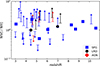 |
Fig. C.1. Observed ratio of N IV] λ1486/N III] λ1750 and 3-σ upper and lower limits for the objects in our sample, as a function of redshift. SFGs, LRDs, and AGN are shown in blue, red, and green, respectively. |
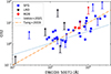 |
Fig. C.2. Extinction-corrected ratio of [O III]λ5007/[O II] λ3727 versus EW of [O III]λ5007 for our sample. Colours as in Fig.C.1. The dash-dotted and dotted lines show the average relations found for SFGs at z ∼ 1 − 2 and low-z by Tang et al. (2019) and Izotov et al. (2021), respectively. |
C.2. SFR and stellar mass surface densities
Using the stellar masses, SFR, and galaxy sizes mentioned earlier (Sects. 3.1, 4.3), we computed the stellar mass and SFR surface densities of the N-emitters for which the data is available. The resulting surface densities are shown in Fig.C.3 and compared to those of normal SFGs at 5 < z < 14 derived by Morishita et al. (2024). We find that N-emitters are not found exclusively at the highest values, in contrast to what was expected by, for example, Schaerer et al. (2024) and Harikane et al. (2025). Most of the objects lie below log(ΣM★) = 3.0 M⊙ pc−2 and log(SFRHα) = 1.0 M⊙ yr−1 kpc−2. Still, a few objects are found among the highest stellar mass and SFR surface densities, including CEERS-1019. This result supports the observed morphologies of the objects in our sample, as shown in Fig.5, indicating that N-emitters are not necessarily compact and are more diverse than previously found.
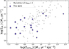 |
Fig. C.3. Stellar mass and SFR surface densities for a subset of 17 new N-emitters for which size measurements and SED parameters are available. The grey points show a comparison sample of z > 5 galaxies from Morishita et al. (2024). |
Appendix D: Abundance determinations
D.1. Metallicity (O/H)
Fig. D.1 shows a comparison of the metallicities obtained with different strong line methods, and our final, adopted metallicity. This complements the text in Sect. 4.1.
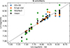 |
Fig. D.1. Metallicity (O/H) comparison using different strong line calibrations and combinations (see text). The adopted metallicity is the mean obtained from different calibrations, shown by black circles. |
D.2. Comments on the determination of CNO abundances
Illustrations providing further details on our abundance determinations are provided here.
In Fig. D.2 we show the correlation between Te([O III]) and the O/H abundance, as derived from auroral line measurements of [O III]λ4363 both in low- and high-z SFGs. A linear fit to the AURORA data (Sanders et al. 2025) yields Te(x) = − 14172.25 * x + 128036.66 K, where x = 12 + log(O/H). We adopt Te([O III]) = max(15000, Te(x)) K for our abundance determinations with ‘variable Te’ in Sect. 4.2.
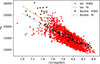 |
Fig. D.2. Te([O III]) versus O/H obtained from the auroral line measurements in the low-redshift sample of Izotov et al. (2021) (red symbols), and JWST spectra of z ∼ 2 − 5 galaxies from Sanders et al. (2025) (black points). The dotted and dash-dotted lines show a linear regression to the two samples. |
For relative N/C abundance, we similarly compute three versions,
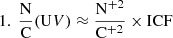 (D.1)
(D.1)
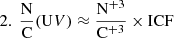 (D.2)
(D.2)
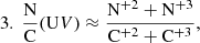 (D.3)
(D.3)
where the last is in practice only applicable to one object where the four necessary lines are detected. For simplicity, we assume all ICF = 1 here. According to the photoionisation models of Martinez et al. (2025), the ICF for N+2/C+2 is between 0.8 − 0.95 for ionisation parameters log(U)∼ − 3 to −1, which represents a small correction (≲0.1 dex).
D.2.1. On the temperature and density dependence of relative CNO abundances
Key for ionic abundance ratio determinations are the line emissivities and their dependence on electron temperature and density, since by definition the abundance of an ion Xi relative to hydrogen, for example, is
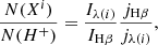 (D.4)
(D.4)
where j denotes the emissivity, I the line intensity, and the Hβ hydrogen line. In the context of N-emitters, this was recently discussed, for example, by Berg et al. (2025) and Arellano-Córdova et al. (2026). For the UV emission lines of interest here, the emissivities depend strongly on the electron temperature Te, leading to considerable uncertainties when Te cannot be measured. For densities sufficiently below the critical density, one has typically
 (D.5)
(D.5)
where t = Te/104, and E4, 20 a term which weakly depends on t, and ci and di are constants for each specific line λ(i) (see e.g. Villar-Martín et al. 2004). For example, for N+3/H+ one has ci = 1.06 × 10⁻⁷ and di = 4.2 for the relative line intensities of N III] λ1750 and Hβ. As Eq. D.5 shows, the emissivity of N III] λ1750 therefore increases rapidly with increasing Te, leading to a lower ionic N+3/H+ abundance. To circumvent this strong temperature dependence, we used the above relative ionic ratios between C, N, and O from UV lines, which all show strong, but comparable temperature dependencies (i.e. large, but similar values of di). For example, the ionic abundance ratio of
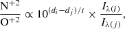 (D.6)
(D.6)
derived from the relative intensities of N III] λ1750 and O III] is then only weakly dependent on Te, since di − dj = −0.18 (cf. Villar-Martín et al. 2004). Also, for N3+/O2+ one has di − dj = 0.45, whereas the relative emissivities between the rest-UV lines of Nitrogen and [O III]λ5007 depend very strongly on Te. And N+2/C+2 and N+3/C+3 also show a weak temperature dependence. In short, relative abundances of CNO elements derived from the UV lines depend only weakly on the (unknown) temperature, whereas abundance ratios involving hydrogen (and/or other combinations of UV and optical lines) are very sensitive to Te, which may also vary across the line-emitting regions.
Regarding the density dependence, the situation is quite simple. All the UV lines of C, N, and O are doublets or multiplets of semi-forbidden lines where at least one of the components has a high critical density (typically ne, crit ∼ 109 − 1010 cm−3, see e.g. Martinez et al. 2025). In practice, as long as the electron density is ne ≲ 109 cm−3 the total emissivity of the N IV] λ1486, N III] λ1750, O III], C III] λ1909 doublets or multiplets (i.e. the sum of the emissivities of all components) is essentially constant, i.e. density-independent (and thus equal to their value at the low-density limit). The same holds for the emissivity of C IVλ1550. Since our PRISM spectra do not resolve the component of these doublets/multiplets, we can therefore easily apply the above equations, and our relative abundances do not depend on the electron density, as long as ne ≲ 109 cm−3.
We used pyneb (Luridiana et al. 2015) and recent atomic data to verify the validity of the above statements. We also compared the analytic expressions from Villar-Martín et al. (2004) with the emissivities obtained with pyneb, finding overall good agreement, and deviations of less than < 20% in some cases, which validates our approach.
Appendix E: Acknowledgements
DS wishes to thank the IAP, Paris, and its staff for their hospitality during a stay where some of this work was done. And many colleagues for interesting discussions on very massive and supermassive stars, and related topics. We also thank Zorayda Martinez for sharing results from her work in electronic format. We thank the numerous teams of the observational programs used in this study, for developing these valuable data sets. The N-emitters identified in this study derive in particular from the following programs: 1180, 1181, 3215 (PI: Eisenstein), 1212, 1214, 1215, 1286 (PI: Luetzgendorf), 1345 (PI: Finkelstein), 1433 (PI: Coe), 2073 (PI: Hennawi), 2561 (PI: Labbe), 4233 (PI: de Graaff), 4446 (PI: Frye), 4598 (PI: Bradac), 5224 (PI: Oesch), 6368 (PI: Dickinson), and 6585 (PI: Coulter) This work is based on observations made with the NASA/ESA/CSA James Webb Space Telescope. The data were obtained from the Mikulski Archive for Space Telescopes at the Space Telescope Science Institute, which is operated by the Association of Universities for Research in Astronomy,Inc., under NASA contract NAS5-03127 for JWST. The data products presented herein were retrieved from the Dawn JWST Archive (DJA). DJA is an initiative of the Cosmic Dawn Center(DAWN), which is funded by the Danish National Research Foundation under grant DNRF140.
All Tables
Significant line detections (≥3σ) listing the number of objects and their separation into SFG, LRD, and AGN types.
N-emitter sample (45+1 objects), including 4 previously known N-emitters from the literature. Note: † AGN. ‡ LRD. * Literature sample.
All Figures
|
Fig. 1. NIRSpec/PRISM spectra of two N-emitters, illustrating the diversity of our sample. Top: Spectrum corresponding to a highly SF galaxy with strong optical lines. Bottom: Spectrum with a Balmer break at ∼3740 Å, a very low EW(Hβ), and faint optical lines. Both spectra show at least one significant UV nitrogen line. |
| In the text | |
|
Fig. 2. Left: Absolute UV magnitude MUV of all known N-emitters (60 in total) vs. redshift. The literature sample is marked with crosses. The colours distinguish objects categorised as SFGs (blue), LRDs (black), and AGNs (red). The literature sample also includes four lensed galaxies, whose magnitudes have been corrected for gravitational lensing. Right: Mass–SFR showing a subset of the N-emitters (symbols colour-coded by redshift) with derived stellar masses, alongside the SF MS of Cole et al. (2025) at z = 7 − 9 (dashed line). |
| In the text | |
|
Fig. 3. Observed properties of N-emitters (SFG in blue, LRD in black, and AGN in red). The EWs of the UV lines (left: N III] λ1750, N IV] λ1486; right: C III] λ1909, C IVλ1550) are shown as a function of EW(Hβ) (top row). Typical error bars are comparable to symbol size and are therefore not shown. Upper limits for N IV] λ1486 and C IVλ1550 are indicated with blue arrows, while the limits for N III] λ1750 and C III] λ1909 are indicated with magenta arrows. The observed correlations of carbon-emitters from Tang et al. (2026) are shown as dotted and dashed lines (for C III] and C IV), for reference also in the top-left panel. Bottom: N IV] λ1486/N III] λ1750 vs. EW(Hβ) and O32 vs. R23. Symbols and colour codes are identical to the main plot. Bottom right: Low-z and high-z data from Izotov et al. (2021) and D’Eugenio et al. (2025). In all panels, 3σ limits are shown. The EWs are in the rest-frame. |
| In the text | |
|
Fig. 4. CNO abundance ratios of the N-emitters (coloured symbols) as a function of metallicity (O/H). Top left: N/O abundances computed using variable Te(O/H); top right: for fixed Te = 22 000 K. The coloured squares show the N/O(UV) values from UV lines only (orange, magenta, and green for Eqs. (1), (2), and (3)). The red diamonds show N/O(UV-opt) derived from UV and optical lines following Eq. (4). Bottom left: N/C and lower limits from UV lines (blue); bottom right: C/O, using same coloured symbols. Low-z SF galaxies and H II regions from the compilation of Izotov et al. (2023) are shown as small black symbols. The dash-dotted lines show the average trends observed in low-z SF galaxies, as parametrised by Vila-Costas & Edmunds (1993) and Nicholls et al. (2017). |
| In the text | |
|
Fig. 5. NIRCam F115W, F356W, and F444W composite 1″ × 1″ images of four N-emitters from our sample, highlighting the morphological diversity within the population, including compact, disky, and clumpy structures. |
| In the text | |
|
Fig. 6. Redshift evolution of the fraction of N-emitters (black diamonds), combining the literature and our sample, among all available NIRSpec PRISM spectra with robust redshifts (grade = 3) from the DJA dataset. The blue lines show the fraction of the rest-UV line emitters 4σ (solid) or 3σ detection (dotted) thresholds, respectively. The red line indicates the fraction of objects with rest-optical emission lines, while the magenta lines indicates all ELGs (UV and/or optical). At z ≳ 11 the number of objects is very small (< 10 per bin), and few objects show emission lines. |
| In the text | |
|
Fig. C.1. Observed ratio of N IV] λ1486/N III] λ1750 and 3-σ upper and lower limits for the objects in our sample, as a function of redshift. SFGs, LRDs, and AGN are shown in blue, red, and green, respectively. |
| In the text | |
|
Fig. C.2. Extinction-corrected ratio of [O III]λ5007/[O II] λ3727 versus EW of [O III]λ5007 for our sample. Colours as in Fig.C.1. The dash-dotted and dotted lines show the average relations found for SFGs at z ∼ 1 − 2 and low-z by Tang et al. (2019) and Izotov et al. (2021), respectively. |
| In the text | |
|
Fig. C.3. Stellar mass and SFR surface densities for a subset of 17 new N-emitters for which size measurements and SED parameters are available. The grey points show a comparison sample of z > 5 galaxies from Morishita et al. (2024). |
| In the text | |
|
Fig. D.1. Metallicity (O/H) comparison using different strong line calibrations and combinations (see text). The adopted metallicity is the mean obtained from different calibrations, shown by black circles. |
| In the text | |
|
Fig. D.2. Te([O III]) versus O/H obtained from the auroral line measurements in the low-redshift sample of Izotov et al. (2021) (red symbols), and JWST spectra of z ∼ 2 − 5 galaxies from Sanders et al. (2025) (black points). The dotted and dash-dotted lines show a linear regression to the two samples. |
| In the text | |
Current usage metrics show cumulative count of Article Views (full-text article views including HTML views, PDF and ePub downloads, according to the available data) and Abstracts Views on Vision4Press platform.
Data correspond to usage on the plateform after 2015. The current usage metrics is available 48-96 hours after online publication and is updated daily on week days.
Initial download of the metrics may take a while.