| Issue |
A&A
Volume 709, May 2026
|
|
|---|---|---|
| Article Number | A81 | |
| Number of page(s) | 6 | |
| Section | Stellar structure and evolution | |
| DOI | https://doi.org/10.1051/0004-6361/202658978 | |
| Published online | 06 May 2026 | |
New single-valued-parameters radiative accelerations of Sc and Ni for modelling stellar interiors
1
LUX, Observatoire de Paris, CNRS, Sorbonne Université, PSL Université, 5 place Jules Janssen, F-92190 Meudon, France
2
Département de physique et d’astronomie, Université de Moncton, Moncton, NB E1A 3E9, Canada
3
IRAP, Université de Toulouse, CNRS, CNES, Toulouse, France
★ Corresponding author: This email address is being protected from spambots. You need JavaScript enabled to view it.
Received:
15
January
2026
Accepted:
15
March
2026
Abstract
Context. The precise evaluation of the radiative accelerations of chemical elements in stars is critical since these accelerations are often the principal contributor to atomic diffusion. Atomic diffusion causes the migration of elements inside stars and therefore affects their structure and evolution. For stellar modelling, the maximum number of elements need to be included, especially for the most abundant species.
Aims. This study presents radiative accelerations of scandium and nickel in stellar interiors. The abundance of scandium is important for identifying AmFm stars, and nickel can contribute strongly to the total opacity at certain depths in stars. Our results for these two elements complement existing tables used to compute radiative accelerations with the single-valued-parameters method; such tables now include up to 12 elements.
Methods. We used the single-valued-parameters method to calculate radiative accelerations. This method simplifies the integration of radiative accelerations in astrophysical codes. It is also more numerically efficient than other calculation methods. The single-valued-parameters method is implemented in three widely used stellar evolution codes.
Results. We present radiative accelerations of scandium and nickel in various stellar models and for different abundances. The parameters needed to evaluate them are made available for main-sequence stars from 1 to 10 solar masses and have been added to our existing publicly available data.
Conclusions. Radiative accelerations calculated here for nickel are comparable to those obtained by the Opacity Project method. According to our results on the radiative accelerations of scandium, calculations that take atomic diffusion into account should explain its underabundances as measured from observations of stars with masses of less than 3 solar masses.
Key words: diffusion / stars: abundances / stars: chemically peculiar
© The Authors 2026
 Open Access article, published by EDP Sciences, under the terms of the Creative Commons Attribution License (https://creativecommons.org/licenses/by/4.0), which permits unrestricted use, distribution, and reproduction in any medium, provided the original work is properly cited.
This article is published in open access under the Subscribe to Open model. This email address is being protected from spambots. You need JavaScript enabled to view it. to support open access publication.
1. Introduction
The calculation of radiative accelerations is an essential ingredient when determining the effects of atomic diffusion processes in stars (Michaud 1970). This process is known to alter the homogenous distribution (outside the stellar core) of chemical elements in the absence of mixing motions. It can occur for certain stellar layers whose position depends on the stellar type and evolutionary stage. Effects of this process are particularly dramatic in the case of chemically peculiar stars, for which extreme abundance anomalies may be observed (see Michaud et al. 2015 for a detailed discussion of atomic diffusion in stars). Also, abundance stratification can affect the structure and evolution of stars. Detailed modeling of atomic diffusion that includes the elements that contribute significantly to the total opacity is critical for certain types of stars.
Computing radiative accelerations is a difficult task, especially for optically thin media (i.e. stellar atmospheres), and always requires huge atomic or opacity databases (with monochromatic opacities for each element), a side effect being the high price to pay in CPU time. For stellar interiors, various methods (summarised in Sect. 1 of Alecian & LeBlanc 2020) have been used to compute radiative accelerations (see also chapter 3 of Michaud et al. 2015). The most flexible and one of the most accurate ways to compute radiative accelerations in stellar interiors (not in atmospheres) was proposed by Seaton (1997), with data and codes publicly available in the framework of the Opacity Project (OP; Seaton et al. 1992), but it is presently limited to 15 metals (only 12 of which have atomic data). We refer to these accelerations as ‘OP radiative accelerations’.
We computed radiative accelerations in the framework of the single-valued-parameters (SVP) approximation (see Alecian & LeBlanc 2020 for the latest version), a parametric method that enables a less precise, but much faster, determination of radiative accelerations (hereafter grad) compared to other methods. Instead of large databases, this method uses very small tables of parameters (called SVP parameters), which are used to compute the grad for all 12 metals for which atomic data are available in the OP atomic database TOPbase (Cunto et al. 1993): C, N, O, Ne, Na, Mg, Al, Si, S, Ar, Ca, and Fe. In addition to the tables of parameters, Alecian & LeBlanc (2020) provide all the data and codes needed to implement the SVP method in existing stellar evolution codes.
It should be noted that Seaton (1997, 2005) provide the data and codes necessary to calculate grad for three other elements (Cr, Mn, and Ni). However, their atomic data were not calculated, and their grad were obtained via extrapolation from isoelectronic sequences (of iron ions for Ni). Their grad accuracy is therefore not well known. Here we are interested in OP radiative acceleration of nickel. Comparisons with other calculations of Ni opacities made by Turck-Chièze et al. (2013, 2016) show that the Ni OP spectra can, under certain conditions, depart strongly from those based on other calculations and measurements. Since the SVP method explicitly requires atomic data for each ion to prepare the tables of parameters (see Sect. 2), Ni was not included in the latest version of the tables provided by Alecian & LeBlanc (2020). However, Ni contributes significantly to opacity in stellar interior modelling, so knowledge of its abundance distribution in certain stellar layers is important, namely the so-called Z bump around log T ≃ 5.3. We therefore consider it worthwhile to find a way to include Ni parameters in SVP tables. This is the first of our objectives. The challenge is to find a method for determining the SVP parameters of Ni from the grad provided by OP instead of relying on atomic data, as we did for the other elements.
Alecian et al. (2013) calculated the grad of scandium after gathering the relevant atomic data on Sc (Massacrier & Artru 2012), mainly using the Flexible Atomic Code, a relativistic program developed by Gu (2008). These detailed atomic data allow the SVP parameters for scandium to be determined. Despite this possibility, Sc was still not included in the most recent version of the tables published by Alecian & LeBlanc (2020). This time, the reason was the authors’ choice to provide homogeneous tables: their published tables were obtained in the same way for the 12 elements mentioned above, i.e. from TOPbase atomic data, and by correcting some of the parameters using a fitting process with OP grad values, which was not possible for Sc. Since the surface underabundance of Sc is a criterion used to discriminate Am stars, the second objective of this work was to add this element to the SVP tables. The data for Sc and Ni will be included in the next release of the data needed for the SVP method.
In Sect. 2 we discuss SVP approximations in the context of this work. In Sect. 3 we propose our method for determining the SVP parameters of nickel from the OP radiative accelerations. Section 4 is devoted to the parameters for scandium. A discussion and our conclusions are presented in Sect. 5.
2. The SVP method
The SVP approximation is presented in detail by Alecian & LeBlanc (2002) and LeBlanc & Alecian (2004). Here, we only discuss grad due to bound-bound (b-b) transitions (the main contributor to grad). In a nutshell, this approximation consists of determining for each ion i the four parameters ( ,
,  ,
,  , and αi) entering the following formula:
 (1)
(1)
where q and p (see below) are factors that depend on the local plasma conditions. Ci is the concentration (in numbers) of the ion (i) relative to hydrogen. Notice that in this expression, the concentration Ci is separated from the other terms, which mainly depend on atomic data and local plasma conditions.
The factors q and p are given by Eqs. (2) and (3) of Alecian & LeBlanc (2020):
 (2)
(2)
and
 (3)
(3)
The quantities Teff and R are the effective temperature and radius of the star, while T and r are the local temperature and radius. The variable Ne is the density (in numbers) of electrons, XH the hydrogen mass fraction, and A the atomic mass (in atomic units) of the considered species.
The first three of these parameters ( ,
,  , and
, and  ) were obtained from b-b atomic-transition data at the depth where each ion has its maximum relative population. The parameter
  depends on the oscillator strengths of the atomic transitions of ion i, while
  depends on their line widths. This last parameter determines in large part the saturation effects. The parameter
  also regulates saturation but only comes into play at large abundances. More details concerning these parameters are given below.
The fourth parameter is the exponent αi, which characterizes the dominant line-broadening process and its saturation. For instance, when one considers a unique absorption line with a pure Lorentzian profile, αi = −0.5. In real cases, there are numerous lines with Voigt profiles at various stages of saturation. When determining a real αi, one first sets its value to −0.5 (a default value); in a second step, this value is adjusted to a more precise estimate of grad (presently, those provided by the OP).
Two additional parameters (ai and bi) have been added to correct the contribution of photoionisation to grad (see Eqs. 5 and 9 of LeBlanc & Alecian 2004). By default, they can be set to 1 and 0, respectively.
Strictly speaking, all six parameters depend on the stellar model. However, they depend very weakly on the effective temperature (and the star’s mass). Thus, a small number of sets of SVP tables are sufficient to cover most stellar types of the main sequence. Practically, 17 tables (around 350 kilobytes in total) are sufficient to calculate grad for 14 metals (12 elements with OP atomic data plus Ni and Sc) and for any main-sequence star through a simple interpolation method between tables of SVP parameters calculated for models of 1–10 solar masses (Alecian & LeBlanc 2020). The SVP method has been applied in several stellar evolution codes. Théado et al. (2009) incorporated the SVP method in the TGEC code (Richard et al. 2004; Hui-Bon-Hoa 2008). It was also added to the CESAM2k20 code (Marques et al. 2013; Manchon et al. 2025) by Deal et al. (2018). More recently, the SVP method was included in Moedas et al. (2025)’s version of the MESA code (Paxton et al. 2011, 2013).
The SVP method has recently been compared by Hui-Bon-Hoa (2024) to the one proposed by the OP (version OPCD3.3; Seaton 2005) for stellar interiors (for stars with 1.5, 2.0, and 2.5 solar masses). Hui-Bon-Hoa (2024) find that the two methods give similar surface abundance time variations in evolution models.
In the present context,  can be neglected1 and set to zero, and the approximate formulae for the SVP approximation for the contribution of b-b transitions can be written in a reduced form as
 (4)
(4)
where only three parameters are involved.
3. Determining the SVP parameters for nickel
We explained in Sect. 1 why, in the absence of detailed data on nickel atomic transitions from the OP, the relevant parameters could not be included in the SVP tables as was done for the other 12 metals. However, the OP provides estimates of Ni grad for any concentration, which enabled us to determine the SVP parameters for this element that give more or less the same accelerations as the OP. Hereafter, to avoid any confusion between the normal SVP method (parameters computed from atomic data) and the reverse method (parameters deduced from grad), we refer to the latter as the rSVP method. To prepare and validate our rSVP method, we applied it to iron, for which all atomic data are in TOPbase, but to mimic the Ni case we assumed that they did not exist in the database. Applying the rSVP method to iron, we finally obtained satisfactory values for these three parameters. Though their values are not exactly the same as those obtained by Alecian & LeBlanc (2020), who provide the full six parameters, the grad values obtained with rSVP are quite accurate (typical discrepancies of less than 0.1 dex for grad, and never more than 0.2 dex), at least for abundances from 0.1 to 10 times the solar abundance of Fe (a smaller interval than with SVP).
On the other hand, both methods deal with ions, and not with an element as a whole. Therefore, the relative populations of all nickel ions must be calculated. This was done by applying the Saha-Boltzmann equations, using the (simplified) grouped energy level tables and codes that are included in the downloadable package published by Alecian & LeBlanc (2020). Since the energy levels of Ni are not in TOPbase, we estimated them from a provisional atomic database kindly provided by F. Delahaye (2018, private communication).
In this work we used the same 17 stellar models as Alecian & LeBlanc (2020). They were computed with the evolution code CESAM2k20, which is identical to the CESTAM models kindly communicated by M. Deal (Marques et al. 2013; Deal et al. 2018). We recall that these models concern stars with masses from 1 to 10 solar masses and are at about the middle of their life on the main sequence.
3.1. Determination of 
This parameter is certainly the easiest one to determine, since it is given by the following simple expression:
 (5)
(5)
where gi, 0 is the grad when the abundance of the element tends to zero2. We recall here the general behaviour of grad due to a single atomic line as a function of the concentration of the ion (as discussed in Alecian & LeBlanc 2000). In Fig. 1a we present γrad, which is the dimensionless normalized grad, as a function of the dimensionless normalized concentration, X3. In Fig. 1b we present the logarithmic derivative of γrad with respect to X, which is related to α. The use of dimensionless normalized quantities allows us to highlight the typical behaviour of grad independently of the specific properties of the line (see details in Alecian & LeBlanc 2000).
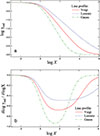 |
Fig. 1. Behaviour of grad for a single atomic line with respect to the relative concentration of the considered ion (see text). The dashed line is for a Lorentzian profile (α = −0.5), the dash-dotted line is the approximation for a Gaussian profile (α = −1.0), and the continuous line mimics the case of a Voigt profile (α = −0.7). Panel (a): γrad (the dimensionless normalized grad) vs X (the logarithm of the dimensionless normalized concentration). Panel (b): Logarithmic derivative of γrad. The minimum value is close to the exponent α. The increase in the derivative after the minimum depends on the value assumed for the contribution of photoionisation to grad; here it is set to 10−3 (see details in Alecian & LeBlanc 2000). |
To obtain this parameter, we just had to compute gi, 0 with the OP values, i.e. the grad(Ni) for a very small abundance of Ni4. We verified that a concentration of 10−6 times the solar abundance is sufficient (which corresponds to X < −2 in Fig. 1). An example of the result is shown in Fig. 2 for a 2.0 solar mass star on the main sequence. The discrepancy is generally smaller than 0.2 dex (and typically less than 0.1 dex) except around log T = 6.1, where NiXIX, which is in a rare-earth configuration, becomes dominant.
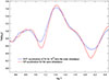 |
Fig. 2. Comparison of rSVP and OP accelerations for 10−6 times the solar abundance of Ni, for a 2.0 solar mass star on the main sequence. The logarithm of the acceleration (in cm.s−2) is plotted versus log T(K). |
3.2. Determination of αi
Before determining  (which is discussed in Sect. 3.3), we needed to estimate αi. We recall that this exponent indicates how grad depends on the ion concentration when transition lines saturate.
The bottom panel of Fig. 1 shows the theoretical variation in αi (or the derivative of the dimensionless grad) with respect to the (dimensionless) concentration when one considers a single absorption line. This exponent reaches a minimum value of between approximately −1 < α < −0.5 for a given concentration. An exponent value of −1 corresponds to a pure Gaussian profile, and −0.5 to a pure Lorentzian profile; the case of a Voigt profile is also shown as an example. At small concentrations, Fig. 1b shows how α tends to zero for a completely unsaturated line, decreases with increasing concentration and reaches a minimum, and then increases again, approaching zero when the grad from photoionisation (which is much less sensitive to element concentration) starts to dominate the line contribution to grad (a line contribution decreases when saturation increases). However, a real αi is also shown (for FeXI and XIII) in Fig. 6 of Alecian & LeBlanc (2000), where we see that, if a first minimum appears as expected, the evolution of grad for higher concentrations is very different: αi starts to increase after the first minimum and decreases again for very high concentrations. The reason for the discrepancies between theoretical and real αi is quite understandable, since the real αi is obtained numerically (from the OP for instance), which involves a large collection of absorption lines at various stages of saturation, and depends on the stellar interior model used (as well as on the effect of the overall chemical composition when the concentration of the element in question varies, particularly when extreme overabundances are imposed).
In the SVP method, α is first set to -0.5 for each ion, and then in a second step is adjusted with an iterative procedure that confronts the grad given by SVP to those from the OP. The final set of parameters for a given element is the one that yields the closest grad to the OP value. In the case of the rSVP method, we chose to numerically compute the derivative of grad for Ni from the OP with respect to its concentration (this derivative is proportional to α) and considered how it varies as a function of concentration. An example is shown in Fig. 3, where this parameter is plotted versus the Ni concentration. One can see that the first minimum appears for a large concentration of more than 100 times the solar abundance (another minimum exists for a much higher concentration, for the same reasons as in the previous discussion concerning the real αi). We determined that this first minimum of αi is the best value to use to estimate the saturation effect on grad due to b-b transitions.
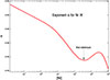 |
Fig. 3. Exponent α of Ni IX at the layer where the population of this ion is at its maximum (log(T)≈5.3) in the 2.0 solar mass model vs the concentration of Ni (in units of solar value). |
3.3. Determination of 
Determining  is more problematic. This parameter, along with αi, determines the effect of absorption line saturation on grad. In the SVP method, it is obtained at a particular concentration, Ci, S, which is determined from atomic-transition data that are not available for Ni (Eq. 14 of Alecian & LeBlanc 2002). It should be noted that Ci, S is proportional to the square value of
  .
.
For the layer where an ion (i) has its maximum relative population, the grad – which is the sum of the acceleration due to b-b transitions (gline) and that due to bound-free transitions (gcont) as given by the OP – can be written as
 (6)
(6)
where  is obtained from our Eq. (4) and
  from Eq. 4 of LeBlanc & Alecian (2004). As a reminder, in the SVP method, Ci, S is obtained from atomic-transition data. Since these data are missing for Ni, a new way to estimate its value is needed. The physical meaning of Ci, S is the ion concentration above which the saturation of lines becomes significant. This definition is clearly too vague to be used to determine
  via the rSVP method. However, it does suggest that Ci, S should be lower than the concentration where the first minimum of α appears in Fig. 3. We therefore adopted an empirical approach by searching for the Ci, S (which must be lower than the value giving the first minimum of α) that yields the rSVP acceleration closest to that of the OP. To avoid confusion with the one obtained through atomic data, we call this particular concentration
  . From Eqs. (4) and (6), assuming concentration
  and using the
  and αi found in the previous sections, we have
![Mathematical equation: $$ \begin{aligned} {{\psi }}_{i}^{*}{=}{\left({\frac{{C}_{i,S}^{^{\prime }}}{p}}\right)}^{1/2}\times {\left[{{\left({\frac{{g}_{\rm {rad}}{-}{g}_{i,\mathrm {cont}}}{q{\varphi }_{i}^{*}}}\right)}^{1/{\alpha }_i}-{1}}\right]}^{-1/2}. \end{aligned} $$](/articles/aa/full_html/2026/05/aa58978-26/aa58978-26-eq28.gif) (7)
(7)
Trying several concentrations for  , we found that adopting the concentration that yields the first minimum of αi and dividing it by 3 provides the best fits with the OP grad. For models with stellar masses higher than 4.5 solar mass, better fits are obtained when this concentration is divided by 4 instead of 3.
3.4. Comparison of Ni radiative accelerations from the OP and the rSVP method
We compare the Ni grad from the OP to those determined via the rSVP method (using the rSVP parameters defined above) in Fig. 4 for a 2 solar mass star on the main sequence (the CESAM2k20 model). Radiative accelerations are shown for various Ni abundances. Note that the same set of parameters is used for these four abundances. We see that the discrepancies are smaller than 0.2 dex and often less than 0.1 dex. The largest discrepancies are found near the minima of the acceleration and are caused by the domination of noble gas configuration ionisation stages. This is because the parameters of the SVP approximation are determined by assuming that when an ion of charge i reaches its maximum relative population, it becomes the main contributor to grad. When the grad of ion i has a low acceleration, as in the case of a noble gas configuration, it is more sensitive to the acceleration of neighbouring ions (of charge i − 1, i + 1), and therefore this assumption is less robust.
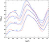 |
Fig. 4. Radiative acceleration of nickel for a 2.0 solar mass star on the main sequence. Curves in red are OP accelerations, and blue lines are those obtained with rSVP parameters. Accelerations are shown for four abundances of Ni: 0.1, 1, 10, and 100 times the solar abundance. |
For models with other masses, we find similar differences between the two methods, and the same kinds of tendencies. We thus conclude that the grad given by the rSVP method are similar to those of the OP.
4. The case of scandium
Scandium is an important element to take into consideration when studying Am stars because it is one of the two metals (with calcium) that are almost systematically deficient in these stars (e.g. Conti 1970). Therefore, any set of physical processes invoked in modelling the Am star phenomenon must explain the observed Sc underabundance.
As mentioned in Sect. 1, Alecian et al. (2013) calculated the grad of scandium for chemically peculiar Am stars using the Sc atomic data from Massacrier & Artru (2012). Therefore, we have what is necessary to compute its grad and, therefore, its SVP parameters for the 17 main-sequence models used for Ni and for the 12 other metals from TOPbase. However, since this element is not available in TOPbase, we cannot improve its parameters through the fitting process as proposed by Alecian & LeBlanc (2020). Hence, the SVP parameters used in the present work were obtained directly from the equations of Alecian & LeBlanc (2002).
The grad values of Sc obtained for our 17 models are shown in Fig. 5. They were all computed for a solar abundance of Sc. The curve (thick solid red line) for the 2.0 solar mass model is highlighted in this figure because it corresponds to a typical Am star and is close to the one (1.9 solar mass) considered by Alecian et al. (2013). This grad curve differs slightly from the one published by Alecian et al. (2013) due to the fact that the models are not strictly identical, but also because some major improvements were done in 2016 in the way the OP monochromatic opacities are managed in our code to compute the SVP parameters5. Another curve is highlighted (the thick solid black line representing grad for the 3.0 solar mass model) because it corresponds to the stellar mass above which grad(Sc) is found to always be larger than the absolute value of the ‘effective gravity’, geff6. Note that the weakness of grad around log T ≈ 4.6 and 5.8 is due to the Ar-like and Ne-like configurations of the Sc ion. Such drops in grad may explain the underabundances of Sc observed in Am stars (see the discussion in Alecian et al. 2013), but detailed time-dependent diffusion models are needed to confirm this assertion.
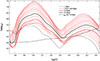 |
Fig. 5. Radiative acceleration of scandium at solar abundance, and for 1.0 to 10.0 solar masses. Some of these curves are highlighted (see the main text for an explanation). The dashed black curve (geff) is the absolute value of gravity plus acceleration due to thermal diffusion for the 3 solar mass model. |
5. Discussion and conclusions
The main goal of this work was to propose a new version of the SVP codes and parameters that extends to scandium and nickel. These two elements are of specific interest for studying the effects of atomic diffusion in main-sequence stars. Scandium underabundance is an important signature of chemically peculiar Am-type stars, and nickel contributes significantly to opacity in the same stellar layers where the ‘iron bump’ phenomenon occurs, a crucial factor for stellar modelling of many types of stars.
The most challenging aspect of this work was determining a reverse procedure (rSVP) to obtain the SVP parameters of nickel from OP grad, rather than from atomic-transition data. We succeeded in determining a set of SVP parameters that allows SVP approximations to be applied to the calculation of grad(Ni) with acceptable accuracy, that is, sufficiently close to the accuracy (albeit within a narrower abundance range) obtained for elements for which atomic-transition data are available. This rSVP method can be used for other elements in the future, for example if, as with nickel, grad values are calculated using other methods but without publicly available atomic-transition data.
Regarding scandium, atomic-transition data are available, but not from the OP database (TOPbase). There are also no grad values in the OP. In this work we calculated the SVP parameters of scandium for stars with masses between 1 and 10 solar masses using atomic data gathered by Massacrier & Artru (2012) and equations of the SVP approximations. These sets of parameters have been included in the SVP tables. However, we cannot improve them using the same fitting procedure as for elements for which OP grad values are available. These parameters should therefore be assumed to be less well adjusted than those previously released for the 12 OP metals for which OP atomic data and grad are available. Nevertheless, they allowed us to calculate the grad of scandium for the 17 CESAM2k20 models, and we have shown that scandium underabundances can be explained for stars with masses of less than 3 solar masses, which is consistent with what is observed in Am stars (Smith 1996); see scenarios A and B in Alecian et al. (2013), which explain the Sc underabundances.
Data availability
All the updated source codes (written in Fortran 90) and the new release of data, now including SVP parameters for 14 metals (C, N, O, Ne, Na, Mg, Al, Si, S, Ar, Ca, Sc, Fe, and Ni) can be downloaded from the websites http://gradsvp.obspm.fr and https://doi.org/10.5281/zenodo.1906888 (detailed instructions are in the READme file). The SVP data needed to calculate the grad of all the metals found in the OP, except for Mn and Cr, are now available on these websites in addition to Sc, which is not in the OP. We plan to apply the rSVP method to these elements in a future work.
Acknowledgments
We would like to thank Morgan Deal for having provided the stellar models used in this paper, and that are available in the numerical package of data and codes of our website http://gradsvp.obspm.fr. We also thank Franck Delahaye for providing atomic data for nickel. This work was supported by a grant from the Natural Sciences and Engineering Research Council of Canada.
References
- Alecian, G., & LeBlanc, F. 2000, MNRAS, 319, 677 [Google Scholar]
- Alecian, G., & LeBlanc, F. 2002, MNRAS, 332, 891 [NASA ADS] [CrossRef] [Google Scholar]
- Alecian, G., & LeBlanc, F. 2020, MNRAS, 498, 3420 [NASA ADS] [CrossRef] [Google Scholar]
- Alecian, G., LeBlanc, F., & Massacrier, G. 2013, A&A, 554, A89 [NASA ADS] [CrossRef] [EDP Sciences] [Google Scholar]
- Conti, P. S. 1970, PASP, 82, 781 [NASA ADS] [CrossRef] [Google Scholar]
- Cunto, W., Mendoza, C., Ochsenbein, F., & Zeippen, C. J. 1993, A&A, 275, L5 [NASA ADS] [Google Scholar]
- Deal, M., Alecian, G., Lebreton, Y., et al. 2018, A&A, 618, A10 [NASA ADS] [CrossRef] [EDP Sciences] [Google Scholar]
- Gu, M. F. 2008, Can. J. Phys., 86, 675 [NASA ADS] [CrossRef] [Google Scholar]
- Hui-Bon-Hoa, A. 2008, Ap&SS, 316, 55 [Google Scholar]
- Hui-Bon-Hoa, A. 2024, A&A, 691, A266 [NASA ADS] [CrossRef] [EDP Sciences] [Google Scholar]
- LeBlanc, F., & Alecian, G. 2004, MNRAS, 352, 1329 [NASA ADS] [CrossRef] [Google Scholar]
- Manchon, L., Deal, M., Marques, J. P. C., & Lebreton, Y. 2025, A&A, 704, A79 [Google Scholar]
- Marques, J. P., Goupil, M. J., Lebreton, Y., et al. 2013, A&A, 549, A74 [NASA ADS] [CrossRef] [EDP Sciences] [Google Scholar]
- Massacrier, G., & Artru, M.-C. 2012, A&A, 538, A52 [NASA ADS] [CrossRef] [EDP Sciences] [Google Scholar]
- Michaud, G. 1970, ApJ, 160, 641 [Google Scholar]
- Michaud, G., Charland, Y., Vauclair, S., & Vauclair, G. 1976, ApJ, 210, 447 [Google Scholar]
- Michaud, G., Alecian, G., & Richer, J. 2015, Atomic Diffusion in Stars, Astronomy and Astrophysics Library (Switzerland: Springer International Publishing) [Google Scholar]
- Moedas, N., Deal, M., & Bossini, D. 2025, A&A, 695, A9 [NASA ADS] [CrossRef] [EDP Sciences] [Google Scholar]
- Paxton, B., Bildsten, L., Dotter, A., et al. 2011, ApJS, 192, 3 [Google Scholar]
- Paxton, B., Cantiello, M., Arras, P., et al. 2013, ApJS, 208, 4 [Google Scholar]
- Richard, O., Théado, S., & Vauclair, S. 2004, Sol. Phys., 220, 243 [Google Scholar]
- Seaton, M. J. 1997, MNRAS, 289, 700 [NASA ADS] [CrossRef] [Google Scholar]
- Seaton, M. J. 2005, MNRAS, 362, L1 [Google Scholar]
- Seaton, M. J., Zeippen, C. J., Tully, J. A., et al. 1992, Rev. Mex. Astron. Astrofis., 23 [Google Scholar]
- Smith, K. C. 1996, Ap&SS, 237, 77 [NASA ADS] [CrossRef] [Google Scholar]
- Théado, S., Vauclair, S., Alecian, G., & LeBlanc, F. 2009, ApJ, 704, 1262 [Google Scholar]
- Turck-Chièze, S., Gilles, D., Le Pennec, M., et al. 2013, High Energy Density Phys., 9, 473 [Google Scholar]
- Turck-Chièze, S., Le Pennec, M., Ducret, J. E., et al. 2016, ApJ, 823, 78 [CrossRef] [Google Scholar]
This parameter provides a correction in the case of a very high overabundance of the considered element; see the comment at the end of Sect. 3.1 in Alecian & LeBlanc (2020).
Actually, it is enough to consider a concentration such that all the absorption lines of the element are unsaturated.
In short, X is obtained by dividing the concentration by the quantity Ci, S (discussed in Sect. 3.3), and γrad is such that it tends towards 1.0 when the concentration of the ion in question becomes zero.
Note that for very small concentrations, the contribution of photoionization to grad can be safely neglected. Therefore, one can consider that the acceleration obtained by the OP for very small concentrations is almost equal to the contribution of b-b transitions alone.
The background monochromatic opacities now enter the calculation of SVP parameters.
Effective gravity is the gravity plus the acceleration due to thermal diffusion as proposed by Michaud et al. (1976, see their Eq. 8) and used by Alecian et al. (2013) to determine the stellar layers where Sc is not supported by grad.
All Figures
|
Fig. 1. Behaviour of grad for a single atomic line with respect to the relative concentration of the considered ion (see text). The dashed line is for a Lorentzian profile (α = −0.5), the dash-dotted line is the approximation for a Gaussian profile (α = −1.0), and the continuous line mimics the case of a Voigt profile (α = −0.7). Panel (a): γrad (the dimensionless normalized grad) vs X (the logarithm of the dimensionless normalized concentration). Panel (b): Logarithmic derivative of γrad. The minimum value is close to the exponent α. The increase in the derivative after the minimum depends on the value assumed for the contribution of photoionisation to grad; here it is set to 10−3 (see details in Alecian & LeBlanc 2000). |
| In the text | |
|
Fig. 2. Comparison of rSVP and OP accelerations for 10−6 times the solar abundance of Ni, for a 2.0 solar mass star on the main sequence. The logarithm of the acceleration (in cm.s−2) is plotted versus log T(K). |
| In the text | |
|
Fig. 3. Exponent α of Ni IX at the layer where the population of this ion is at its maximum (log(T)≈5.3) in the 2.0 solar mass model vs the concentration of Ni (in units of solar value). |
| In the text | |
|
Fig. 4. Radiative acceleration of nickel for a 2.0 solar mass star on the main sequence. Curves in red are OP accelerations, and blue lines are those obtained with rSVP parameters. Accelerations are shown for four abundances of Ni: 0.1, 1, 10, and 100 times the solar abundance. |
| In the text | |
|
Fig. 5. Radiative acceleration of scandium at solar abundance, and for 1.0 to 10.0 solar masses. Some of these curves are highlighted (see the main text for an explanation). The dashed black curve (geff) is the absolute value of gravity plus acceleration due to thermal diffusion for the 3 solar mass model. |
| In the text | |
Current usage metrics show cumulative count of Article Views (full-text article views including HTML views, PDF and ePub downloads, according to the available data) and Abstracts Views on Vision4Press platform.
Data correspond to usage on the plateform after 2015. The current usage metrics is available 48-96 hours after online publication and is updated daily on week days.
Initial download of the metrics may take a while.