| Issue |
A&A
Volume 709, May 2026
|
|
|---|---|---|
| Article Number | A162 | |
| Number of page(s) | 11 | |
| Section | Cosmology (including clusters of galaxies) | |
| DOI | https://doi.org/10.1051/0004-6361/202658945 | |
| Published online | 13 May 2026 | |
A new magnitude–redshift relation based on Type Ia supernovae
1
Pontificia Universidad Católica de Chile, Vicuña Mackenna, 4860 Macul, Santiago, Chile
2
Instituto Milenio de Astrofísica (MAS), Nuncio Monseñor Sótero Sanz 100, Of. 104, Santiago, Chile
★ Corresponding author: This email address is being protected from spambots. You need JavaScript enabled to view it.
Received:
13
January
2026
Accepted:
2
March
2026
Abstract
We present a new empirical relation between the standardised magnitude (m) of Type Ia supernovae (SNe Ia) and redshift (z). Using the Pantheon+ sample and the Dark Energy Survey (DES) five-year sample (DES-SN5YR), we find a negative linear correlation between m − 5log(z(1 + z)) and z, implying that their magnitude–redshift relation can be parametrised with just two parameters: an intercept ℳ and a slope b. This relation corresponds to the luminosity distance dL(z) =c H0−1z(1 + z)10bz/5 and is valid up to at least z ≃ 1.1. It outperforms the ΛCDM and flat wCDM models and the (2,1) Padé approximant for dL(z), and performs comparably to the flat ΛCDM model and the (2,1) Padé(j0 = 1) model of Hu et al. Furthermore, the relation is relatively stable in the absence of low-z SNe, making it suitable for fitting Hubble diagrams of SNe Ia without adding a low-z sample. In deep fields, assuming that the large-scale density is independent of the comoving radial coordinate, b ∝ q0 + 1. We fitted the empirical relation to Hubble diagrams of eight deep-field regions and find no evidence for anisotropy. The inferred q0 values, ranging from −0.6 to −0.4, are consistent within 1.6σ and significantly lower than zero, indicating statistically consistent cosmic acceleration across all eight regions. We applied the empirical relation to the DES-Dovekie and Amalgame SN samples and find b values consistent with those from DES-SN5YR and Pantheon+. Finally, using the empirical relation in the hemispheric comparison method applied to Pantheon+ up to z = 1.1, we find no evidence for anisotropies in ℳ and b.
Key words: supernovae: general / cosmological parameters / cosmology: theory
© The Authors 2026
 Open Access article, published by EDP Sciences, under the terms of the Creative Commons Attribution License (https://creativecommons.org/licenses/by/4.0), which permits unrestricted use, distribution, and reproduction in any medium, provided the original work is properly cited.
This article is published in open access under the Subscribe to Open model. This email address is being protected from spambots. You need JavaScript enabled to view it. to support open access publication.
1. Introduction
General relativity and the assumption of homogeneity and isotropy of the Universe at large scales are two of the foundations of modern cosmology. The latter leads to the Friedmann–Lemaître–Robertson–Walker (FLRW) metric, under which Einstein’s field equations reduce to the Friedmann equations. The first, combined with the FLRW metric, provides a formula for the luminosity distance–redshift relation, dL(z), in terms of three parameters: the Hubble constant (H0), the matter density (ΩM), and the cosmological constant (Λ) with density parameter ΩΛ.
Using Hubble diagrams of Type Ia supernovae (SNe Ia), Riess et al. (1998) and Perlmutter et al. (1999) found ΩΛ > 0 and a deceleration parameter q0 < 0, indicating that the Universe’s expansion is currently accelerating. In this context, Λ is interpreted as a constant dark energy density that drives cosmic acceleration. Given that models with Λ, when fitted to various observational data, yield ΩΛ > 0 (Weinberg et al. 2013), the existence of dark energy is widely accepted, consolidating the Λ cold dark matter (ΛCDM) model as the standard model.
Despite its ability to fit observations, the ΛCDM model has problems of fine-tuning, cosmic coincidence, and tensions in cosmological parameters measured with independent experiments (Perivolaropoulos & Skara 2022; Efstathiou 2025). These issues motivate alternative gravitational theories that explain cosmic acceleration without Λ (Koyama 2016; Odintsov et al. 2025). Moreover, cosmic acceleration may be partly an apparent effect associated with the assumption of homogeneity and isotropy and the corresponding use of the FLRW metric (Räsänen 2006; Enqvist 2008; Wiltshire 2009).
Cosmography provides a model-independent framework to study cosmic acceleration, expressing dL(z) in terms of spatial curvature and kinematic parameters, such as H0, q0, and the jerk parameter (j0). However, this approach relies on the assumption of a homogeneous and isotropic Universe (Hu & Wang 2022).
Among current SN Ia samples, such as Pantheon+ (Brout et al. 2022) and the full five-year sample from the Dark Energy Survey Supernova (DES-SN) program (DES-SN5YR; Sánchez et al. 2024), a significant fraction of SNe originates from deep-field surveys. Analysing deep fields separately allows one to infer direction-dependent parameters without requiring global homogeneity and isotropy. In particular, comparing deep fields across different directions provides a test of isotropy.
Since angular variations in deep fields are expected to be negligible, and assuming that the large-scale density within each field is independent of the comoving radial coordinate, the metric can be approximated as FLRW on a field-by-field basis. Under this assumption, we can measure q0 for each deep field using the FLRW metric, without assuming global homogeneity and isotropy. The main limitation of this approach is the small number of low-z SNe Ia (z < 0.1) in deep fields, which are crucial for breaking parameter degeneracies (Linder 2006).
An approach to reducing the impact of the lack of low-z SNe on the estimation of q0 is to use a dL(z) relation with as few parameters as possible. In the flat ΛCDM model, dL(z) depends only on H0 and ΩM. The latter, which is used to measure q0, remains relatively stable in the absence of low-z SNe (Brout et al. 2022). To date, the only other dL(z) relation that accurately fits SN observations with just two parameters is that proposed by Hu et al. (2024a). This relation corresponds to a third-order Padé approximation with H0 and q0 as free parameters, while j0 is fixed to one, as predicted by the flat ΛCDM model (Bochner et al. 2015).
In this work, we introduce an empirical magnitude–redshift relation (m(z)) and the corresponding dL(z) relation, which provides a straightforward quantitative tool to fit Hubble diagrams of SNe Ia up to at least z ≃ 1.1, using only two parameters and without assuming any theoretical model or spatial curvature. This relation is relatively stable in the absence of low-z SNe, making it suitable for studying SN deep fields without the need to add a low-z sample.
The paper is organised as follows. In Sect. 2, we describe the SN samples and define the deep-field regions. In Sect. 3, we present the m(z) relations used to fit Hubble diagrams. In Sect. 4, we present the results, including the new empirical relation, its comparison with five m(z) relations, and its application to the deep-field regions and other samples. In Sect. 5, we discuss the derived j0 values, the search for cosmic anisotropies, and future analyses. We summarise our conclusions in Sect. 6.
2. Data samples
Pantheon+1 contains data from 1550 SNe Ia, drawn from 18 surveys, with 0.001 ≤ z ≤ 2.261. DES-SN5YR2 contains data from 1635 photometrically classified SNe Ia from the DES-SN programme with 0.060 ≤ z ≤ 1.121, and 194 SNe Ia from four surveys with 0.025 < z < 0.093, referred to as the low-z sample.
The Pantheon+ and DES-SN5YR samples provide (i) RA and Dec coordinates; (ii) standardised SN magnitudes (mBcorr, hereafter m), derived from SALT2 (Pantheon+) and SALT3 (DES-SN5YR) light-curve fits and corrected for stretch, colour, host-galaxy mass, and selection bias; (iii) redshifts corrected for the cosmic microwave background (CMB) dipole and peculiar velocities (zHD, hereafter z); and (iv) the covariance matrix (C) to account for statistical and systematic errors.
Following Brout et al. (2022), we selected SNe with z > 0.01 from the Pantheon+ compilation to minimise the impact of peculiar velocities on the derived cosmological parameters. We refer to this subsample as Pantheon+. Because DES-SN5YR introduced several improvements compared with Pantheon+, its m values are not on the same scale. Specifically, there is a constant offset of 0.04 mag between the selection bias corrections in DES-SN5YR and Pantheon+, which does not affect the cosmological results of each separate analysis (Vincenzi et al. 2025). Hence, we analysed both samples separately.
Fig. 1 shows the sky distribution of SNe in Pantheon+ and DES-SN5YR. The SNe with z ≥ 0.4 are concentrated in small regions of the sky, which reflects the location of the SN deep fields. We defined 14 circular regions for Pantheon+ and four for DES-SN5YR, referred to as XY, which contain virtually all SNe with z ≥ 0.4. In this notation, X denotes the closest Galactic pole and Y indicates the rank of proximity to that pole. Table 1 lists the regions, their centres in (RA, Dec), angular radii (θ), the number of SNe within each region, and the corresponding z ranges.
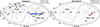 |
Fig. 1. Sky distribution of Pantheon+ and DES-SN5YR SNe. Dashed lines indicate the Galactic equator. Plus and cross symbols mark the north and south Galactic poles, respectively. Circular and triangular regions are also shown. |
Supernova regions.
The S1, S2, S4, and S5 regions in Pantheon+ closely match those in DES-SN5YR. In these regions, DES-SN5YR contains 170–490 more SNe than Pantheon+, while 47–100% of the SNe in the Pantheon+ S1, S2, S4, and S5 regions originate from the DES-SN programme and are already included in DES-SN5YR. Therefore, we used only the DES-SN5YR data for these regions.
The remaining ten Pantheon+ regions contain 13–77 SNe each. To increase the sample while minimising the sky area, we defined the triangular N147, N235, and S367 regions. The N147 region includes N1, N4, N7, and the SNe located within the triangle formed by their centres; the same applies for N235 and S367. For S367, we increased the declination of the centres of S3 and S7 by 1.2° to include more SNe without significantly increasing the area. Fig. 1 shows the triangular regions, while Table 1 lists their barycentres, the number of SNe, and the z ranges. We refer to the S1, S2, S4, S5, N147, N235, S367, and N6 regions as the deep-field regions.
3. Methods
3.1. Magnitude–redshift relations
The m(z) relation for a standard candle with absolute magnitude M is given by
 (1)
(1)
where ℳ = M + 5log(c H0−1 Mpc−1)+25 and 𝒟L(z) =dL(z)H0/c. To derive dL(z) using either a gravitational theory or a cosmographic expansion, we need the metric of the expanding Universe. The simplest choice is the FLRW metric, characterised by the scale factor a and the curvature parameter k. For this metric,
 (2)
(2)
where dM(z) is the transverse comoving distance. Defining H(z) = ȧ/a and Ωk = −kc2/H02, dM(z) is given by
 (3)
(3)
3.1.1. The ΛCDM, flat ΛCDM, and flat wCDM models
In the phenomenological generalisation of the ΛCDM model,
 (4)
(4)
where ΩM + ΩΛ + Ωk = 1 and w is the dark energy equation-of-state parameter. We used the m(z) relations for ΛCDM (w = −1), flat ΛCDM (Ωk = 0, w = −1), and the phenomenological flat wCDM (Ωk = 0) models.
3.1.2. Padé cosmography and flat Padé model
The Padé approximation is a method to approximate a function F(z) as the ratio of two polynomials of orders A and B. The rational function is known as the (A,B) Padé approximant, and its coefficients are expressed in terms of those of the Taylor series of F(z) truncated at order A + B (Baker & Graves-Morris 1996).
Hu & Wang (2022), using Pantheon (Scolnic et al. 2018), report that the (2,1) Padé approximant for dL(z) performs better than cosmographic expansions based on Taylor series. More recently, Hu et al. (2024a) analysed Pantheon+ and found that this approximant outperforms other Padé forms. We therefore adopt it as the best cosmographic approach.
The (2,1) Padé approximant for dL(z) used by Hu et al. (2024a) was derived by Capozziello et al. (2020) for Ωk = 0. To compute the expression valid for any Ωk, we used the third-order Taylor series for dL(z) (Eq. 2 of Cattoën & Visser 2007) and the procedure of Baker & Graves-Morris (1996), obtaining
 (5)
(5)
Here,  , and
, and
 (6)
(6)
For Ωk = 0, Eq. (5) is equivalent to that given in Hu et al. (2024a). We refer to Eq. (5) as the Padé cosmography.
Hu et al. (2024a) also found that the (2,1) Padé approximant for dL(z) with j0 = 1 fixed performs better than the Padé cosmography, the flat ΛCDM, ΛCDM, and flat wCDM models. Since j0 was fixed to unity because this is the value for the flat ΛCDM model, the dL(z) equation proposed by Hu et al. (2024a) is not cosmographic, but rather model-based. We refer to Eq. (5) assuming  as the flat Padé model.
3.1.3. Empirical approach
To fit the Hubble diagram, we introduce the ansatz
 (7)
(7)
where the factor 1 + z is inspired by Eq. (2) and f(z) is a free function that vanishes as z → 0, ensuring dL(z) =cz/H0 at low z. The corresponding m(z) relation is
 (8)
(8)
where the dependence of f(z) on z can be empirically determined from the correlation between m − 5log(z(1 + z)) and z.
3.2. Parameter estimation and model selection
Let v denote the vector with the np free parameters of m(z). The posterior probability of m(z) is P ∝ p(v)ℒ, where p(v) is the prior and ℒ = e−χ2/2. Following Conley et al. (2011),
 (9)
(9)
where Δm is the vector of residuals, whose i-th component is
 (10)
(10)
We assumed non-informative priors; in this case, we obtained the best-fit parameter vector vbest that maximises P by minimising χ2.
To calculate uncertainties, we used EMCEE (Foreman-Mackey et al. 2013), which samples P using a Markov chain Monte Carlo (MCMC) process. First, we defined the priors as flat distributions: ℳ ∈ (23, 25), ΩM ∈ (0, 1), ΩΛ ∈ (0, 1), w ∈ ( − 2, 0), q0 ∈ ( − 2, 1), and  . These priors are wide enough to consider them as uninformative. Next, we initialised 10np walkers in a small Gaussian ball around vbest and ran 105 steps (106 for the flat wCDM model). Then, given an integrated autocorrelation time (τ) provided by EMCEE, we discarded the initial 3τ steps as burn-in and thin by τ/2. With this configuration, we obtain for all parameters a Gelman & Rubin (1992) statistic of
  , indicating convergence of the MCMC chains, and an effective sample size neff > 2000 (neff > 400 for the flat wCDM model). Finally, for each parameter, we adopted the 68.27% confidence interval of its marginalised distribution as the 1σ uncertainty.
To identify which model among a set of candidates best describes the Hubble diagram, we used the corrected Akaike information criterion (AICc; Sugiura 1978) and the Bayesian information criterion (BIC; Schwarz 1978). For each model, we computed AICc = χmin2 + 2npN/(N − np − 1) and BIC = χmin2 + nplnN, where χmin2 = χ2(vbest) and N is the number of SNe. Based on these information criteria (ICs), the preferred model is the one with the lowest IC value (ICmin), and the strength of evidence for each model is given by ΔIC = IC − ICmin. Models with ΔAICc < 2 have substantial support, while those with 4 < ΔAICc < 7 have considerably less support (Burnham & Anderson 2002). Similarly, ΔBIC < 2 indicates little evidence against the model, and 6 < ΔBIC < 10 indicates strong evidence against the model (Kass & Raftery 1995). Therefore, models with both ΔAICc < 2 and ΔBIC < 2 perform comparably, yielding similar fits to the Hubble diagram. Models with larger ΔAICc are progressively less supported, and those with larger ΔBIC are increasingly disfavoured.
4. Results
4.1. Empirical relation
Figure 2 shows m − 5log(z(1 + z)) versus z for Pantheon+ and DES-SN5YR. Their weighted Pearson correlation coefficients (rP; Earp et al. 2019) are close to −0.7, with p-values below 10−220, indicating a moderate-to-strong negative linear correlation. Based on this, we express m − 5log(z(1 + z)) as a linear function of z, with an intercept ℳ and a slope b:
 (11)
(11)
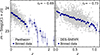 |
Fig. 2. Relation between m − 5log(z(1 + z)) and z for Pantheon+ and DES-SN5YR. Binned data (blue squares) with error bars are shown for visualisation purposes only, both here and throughout the paper. |
Thus, f(z) =bz in Eq. (8), which, together with Eq. (7) yields
 (12)
(12)
We refer to Eqs. (11) and (12) as the empirical relation.
The empirical relation exhibits several characteristics. First, it is relatively stable in the absence of low-z SNe (see Sect. 4.5). Second, its parameters and their associated covariance matrix can be computed analytically. Fig. 3 shows the confidence contours for ℳ and b computed analytically and using EMCEE (using the flat prior b ∈ ( − 2, 0)), which are virtually identical. Third, under the FLRW metric, b ∝ q0 + 1. Indeed, from Eqs. (12) and (2),
 (13)
(13)
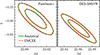 |
Fig. 3. Confidence contours at the 68.27% and 95.45% levels of the empirical relation parameters, obtained analytically and using EMCEE. |
and using Eq. (16) of Li et al. (2020),
 (14)
(14)
which, together with Eq. (6), yields
 (15)
(15)
4.2. Constraints on cosmological parameters
Table 2 lists the parameter constraints from Pantheon+ and DES-SN5YR for the six m(z) relations used in this work. The parameters for the flat ΛCDM, ΛCDM, and flat wCDM models are consistent with those reported by the Pantheon+ team (ΩM = 0.334 ± 0.018 for the flat ΛCDM model, ΩM = 0.306 ± 0.057 and ΩΛ = 0.625 ± 0.084 for the ΛCDM model, and  and w = −0.90 ± 0.14 for the flat wCDM model; Brout et al. 2022) and the DES Collaboration (ΩM = 0.352 ± 0.017 for the flat ΛCDM model,
  and ΩΛ = 0.55 ± 0.10 for the ΛCDM model, and
  and
and  for the flat wCDM model; Camilleri et al. 2024).
Parameter constraints for different magnitude–redshift relations.
For each m(z) relation, the parameters derived from DES-SN5YR and Pantheon+ are consistent within 1σ, except for ℳ, which differs by more than 3.3σ. This discrepancy arises from the constant offset of 0.04 mag between selection bias corrections in DES-SN5YR and Pantheon+ (Vincenzi et al. 2025). After accounting for this offset, the ℳ values derived from DES-SN5YR and Pantheon+ become consistent within 1σ.
4.3. Hubble diagrams and model comparison
Fig. 4 shows the Hubble diagrams for DES-SN5YR and Pantheon+, the best fits for the m(z) relations, and the residuals relative to the empirical relation. For DES-SN5YR, the empirical relation provides a fit comparable to the other m(z) relations. The differences between the m(z) relations and the empirical relation have rms values below 0.009 mag and maximum absolute deviations Δmmax below 0.027 mag. For Pantheon+, the empirical relation begins to diverge from the other m(z) relations at z ≳ 1.4. For z < 1.121 (the highest z in DES-SN5YR), the rms and Δmmax remain below 0.007 and 0.012 mag, respectively.
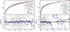 |
Fig. 4. Hubble diagrams of DES-SN5YR and Pantheon+, along with the best-fit m(z) relations. The lower panels show the residuals relative to the empirical relation. |
Given that the empirical relation accurately reproduces the Hubble diagrams of both samples up to z = 1.121, we assume that it is valid at least up to this redshift. Beyond this limit, we cannot reliably assess its validity because Pantheon+ contains only 19 SNe at z > 1.121. In the following, we restrict our analyses of Pantheon+, including its deep-field regions, to z < 1.121, although analyses without this cut lead to the same conclusions. Table 2 lists the parameter constraints for Pantheon+ (z < 1.121).
Table 3 lists the ΔAICc and ΔBIC values. Based on these values, the empirical relation, the flat ΛCDM model, and the flat Padé model provide comparable fits to the Hubble diagrams of DES-SN5YR and Pantheon+ (z < 1.121), with the flat ΛCDM model being only marginally disfavoured for DES-SN5YR (ΔAICc = 2.2 and ΔBIC = 2.1). In contrast, the ΛCDM model, the flat wCDM model, and the Padé cosmography are less supported by the AICc and disfavoured by the BIC, reflecting the penalty associated with their additional free parameter.
AICc and BIC statistics.
4.4. Deceleration parameter and Hubble constant
Table 4 lists the q0 values. For the flat ΛCDM, ΛCDM, and flat wCDM models, we used q0 = ΩM/2 + (1 + 3w)ΩΛ/2. Although developed solely to fit Hubble diagrams, the q0 values of the empirical relation are consistent with those of the other m(z) relations.
Values of q0 for different magnitude–redshift relations.
We estimated H0 using the empirical relation together with Pantheon+ (z < 1.121) and the Cepheid distance moduli (μCeph) from the SH0ES sample (Riess et al. 2022). To do this, we replaced Eq. (10) with Δmi = mi − M − μCeph, i for those SNe hosted in galaxies with μCeph. We obtain M = −19.244 ± 0.030, b = −0.604 ± 0.026, and H0 = 73.4 ± 1.0 km s−1 Mpc−1. This H0 value is consistent with those obtained by Brout et al. (2022) from Pantheon+ and SH0ES, which range from 73.3 ± 1.1 to 73.6 ± 1.1 km s−1 Mpc−1.
4.5. Stability in the absence of low-z SNe
To evaluate the stability of the best-fit parameters of the six m(z) relations in the absence of low-z SNe, we computed ℳ and q0 using SNe with z > zmin, where zmin = 0.01, 0.03, 0.06, 0.10, and 0.15. Fig. 5 shows the resulting (ℳ, q0) points. We find that the empirical relation, the flat ΛCDM model, and the flat Padé model are the most stable in the absence of low-z SNe. Because the best-fit parameters of the empirical relation are the intercept and slope of the approximately linear correlation between m − 5log(z(1 + z)) and z (see Fig. 2 and Eq. (11)), their stability depends primarily on the z baseline of the data. Therefore, they are expected to vary only mildly when low-z SNe are removed.
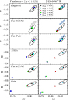 |
Fig. 5. Distribution of q0 versus ℳ for the m(z) relations fitted to DES-SN5YR and Pantheon+ (z < 1.121) with different zmin. Solid curves are the 68.27% confidence contours for zmin = 0.01, while the contour of the empirical relation is shown as a shaded region in each panel for comparison. Although the flat wCDM constraints in the (w, ΩM) plane are highly non-Gaussian, their projection onto q0 leads to nearly symmetric uncertainties, as expected since q0 = QH(z = 0), where the parameter QH(z) is almost free of the w–ΩM degeneracy (Camilleri et al. 2024). |
When fitted to DES-SN5YR, the three most stable relations show a gap between cases with zmin ≥ 0.06 and those with zmin ≤ 0.03. For zmin ≥ 0.06, the selection removes at least 85% of the SNe in the low-z sample of DES-SN5YR. This likely reflects differences in the low-z sample relative to the rest of DES-SN5YR, as also discussed by Huang et al. (2025). This effect does not affect the analysis of the S1, S2, S4, and S5 deep-field regions, as they do not contain any SNe from the low-z sample.
4.6. Deep-field regions
Fig. 6 shows the Hubble diagrams for the deep-field regions. To constrain the parameters of the S1, S2, S4, and S5 regions, we selected the m and z values for the SNe in these regions, along with the corresponding entries of the covariance matrix. We then replaced Eq. (10) with Δmi = mi − m(zi, vj) for the SNe within the j-th region with parameters vj. We applied the same procedure to the S367, N147, N235, and N6 regions. Table 5 lists the parameter constraints for the empirical relation, the flat ΛCDM model, and the flat Padé model. Fig. 6 shows the best fits.
Parameter constraints for the deep-field regions.
Table 6 lists the ΔAICc and ΔBIC values for the empirical relation, the flat ΛCDM model, and the flat Padé model. These values indicate that the three m(z) relations provide comparable fits to the Hubble diagrams in the deep-field regions. Since the empirical relation is purely phenomenological and its parameters, uncertainties, and confidence contours can be computed analytically (Sect. 4.1), we used it as a convenient parametrisation to characterise the deep-field regions.
AICc and BIC statistics for the deep-field regions.
Fig. 7 shows the confidence contours and the marginalised distributions for ℳ and b for the deep-field regions. The b values are consistent within 1.6σ. When accounting for the 0.04 mag offset between the selection bias corrections in DES-SN5YR and Pantheon+, the ℳ values are consistent within 1.6σ, in agreement with isotropy. We obtain similar results when comparing the parameters of the flat ΛCDM and flat Padé models, for which the differences in ℳ, ΩM, and q0do not exceed 1.7σ, 1.5σ, and 1.7σ, respectively.
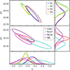 |
Fig. 7. Confidence contours (68.27%) and marginalised distributions of empirical relation parameters fitted to the deep-field regions. |
To test whether fitting the S1, S2, S4, and S5 regions with different parameters for each region (eight parameters in total) provides a significantly better fit than an isotropic fit (two parameters for all regions), we performed a likelihood ratio test (LRT). The test statistic λ = χmin, iso2 − χmin2, where χmin2 is the value for the model with eight parameters (listed in Table 6) and χmin, iso2 is the corresponding value for the isotropic fit, follows a χ2 distribution with six degrees of freedom (Wilks 1938). Fitting the empirical relation, we obtain χmin, iso2 = 1451.3, λ = 8.4, and a p-value of 0.21. For the S367, N235, N147, and N6 regions, we find χmin, iso2 = 383.5, λ = 6.7, and a p-value of 0.35. In both cases, the isotropic fit cannot be rejected. We obtain similar results when using the flat ΛCDM and flat Padé models, for which the LRT p-values lie between 0.20 and 0.36. Therefore, we find no evidence for anisotropy in the Hubble diagrams of the deep-field regions.
Table 7 lists the q0 values for the deep-field regions. The values measured using the empirical relation are consistent within 1.6σ and are lower than zero by more than 4.8σ (99.9998% confidence). These results indicate that the Universe is undergoing accelerated expansion in a statistically consistent manner across all eight deep-field regions, under the assumption that the large-scale densities in these regions are independent of the comoving radial coordinate.
Values of q0 for deep-field regions.
4.7. Application to other samples
4.7.1. DES-Dovekie sample
As this work was nearing completion, Popovic et al. (2025) presented a re-analysis of DES-SN5YR. The resulting recalibrated dataset, DES-Dovekie3, includes improved photometric cross-calibration and a fixed host-galaxy colour law. Since DES-Dovekie supersedes DES-SN5YR (Popovic et al. 2025), its analysis provides the best constraints and overall results from DES-SN combined with a low-z sample.
We fit the empirical relation (b = −0.603 ± 0.020), Padé cosmography ( ,
,  ), flat ΛCDM (ΩM = 0.329 ± 0.015), ΛCDM (
 ,
,  or
or  ), flat wCDM (
 , w = −0.85 ± 0.15), and the flat Padé model (q0 = −0.470 ± 0.022). The parameters are consistent with those derived from DES-SN5YR and Pantheon+ (z < 1.121), as well as with those reported by Popovic et al. (2025) for the flat ΛCDM (ΩM = 0.330 ± 0.015), ΛCDM (ΩM = 0.279 ± 0.057, Ωk = 0.14 ± 0.15), and flat wCDM models (
 ,
,  ). The ΔAICc and ΔBIC values are similar to those obtained for DES-SN5YR.
The magnitude differences between a flat ΛCDM model with ΩM from Planck CMB measurements (ΩMPlanck = 0.3166; Planck Collaboration VI 2020) and the empirical relation have rms = 0.004 mag and a maximum absolute deviation Δmmax = 0.011 mag. In comparison, the empirical relation calibrated with DES-SN5YR and Pantheon+ (z < 1.121) yields (rms, Δmmax) = (0.012, 0.025) for DES-SN5YR and (0.008, 0.014) for Pantheon+. Hence, the empirical relation shows close agreement with the flat ΛCDM model using ΩMPlanck, particularly when calibrated using DES-Dovekie and Pantheon+ (z < 1.121).
For the S1, S2, S4, and S5 regions in DES-Dovekie, the b values are −0.555 ± 0.058, −0.612 ± 0.040, −0.474 ± 0.066, and −0.585 ± 0.036, respectively. These values and those from S367, N147, N235, and N6 are mutually consistent within 1.8 σ. Using an LRT, we obtain λ = 6.6 and a p-value of 0.36, indicating that the isotropic fit cannot be rejected. The corresponding q0 values for S1, S2, S4, and S5 regions are −0.489 ± 0.054, −0.436 ± 0.037, −0.564 ± 0.061, and −0.461 ± 0.033, respectively.
We also constrained parameters using only DES SNe within DES-Dovekie. For this, we selected SNe with z > 0.093, thereby excluding the low-z sample entirely. We obtain b = −0.589 ± 0.026 for the empirical relation, ΩM = 0.307 ± 0.020 for the flat ΛCDM model, and q0 = −0.488 ± 0.029 for the flat Padé model. The corresponding ΔIC values are 0.5, 0.0, and 2.1, indicating that the empirical relation and the flat ΛCDM model provide comparable fits to the Hubble diagram.
4.7.2. Amalgame sample
The Amalgame sample (Popovic et al. 2024)4 consists of 1792 photometrically classified SNe Ia from the Sloan Digital Sky Survey (Sako et al. 2011) and Pan-STARRS1 (Scolnic et al. 2018), spanning 0.066 < z < 0.680. We obtain b = −0.613 ± 0.041 for the empirical relation,  for the flat ΛCDM model, and
  for the flat Padé model. These values are consistent with values obtained from Pantheon+ (z < 1.121), DES-SN5YR, and DES-Dovekie. Fig. 8 shows the Hubble diagram for Amalgame. The ΔIC values for the empirical relation, the flat ΛCDM model, and the flat Padé model are 0.4, 0.0, and 0.6, respectively, showing that all three provide comparable fits to the Hubble diagram.
4.7.3. Baryon acoustic oscillation distances and cosmic chronometers
Although the empirical relation is designed to fit Hubble diagrams of standard candles, we applied it to available dM(z) and H(z) datasets assuming the FLRW metric, which allowed us to transform the empirical relation into expressions for dM(z) (Eq. 13) and H(z) (Eq. 14).
Abdul Karim et al. (2025) reported 13 distance measurements from baryon acoustic oscillations (BAO) in the second data release (DR2) of the Dark Energy Spectroscopic Instrument (DESI), relative to the sound horizon (rd), at effective redshifts zeff ranging from 0.295 to 2.335. These include six dM(z)/rd values, six dH(z)/rd values (with dH(z) =c/H(z)), and one dV(z)/rd value, where dV(z)≡[zdM(z)2dH(z)]1/3. Fitting Eqs. (13) and (14) to the seven BAO distances with zeff < 1.121, and assuming Ωk = 0, we obtain b = −0.584 ± 0.016. For comparison, the b values obtained from Pantheon+ (z < 1.121), DES-SN5YR, DES-Dovekie, and Amalgame, when all SN samples are restricted to z ≥ 0.295, are −0.697 ± 0.050, −0.622 ± 0.035, −0.618 ± 0.033, and −0.688 ± 0.070, respectively. Compared to the BAO constraint, the latter three values are consistent within 1.4σ, while the Pantheon+ (z < 1.121) result is marginally consistent, showing a 2.2σ difference.
Alfano et al. (2026) collected 34 H(z) values measured with cosmic chronometers, spanning 0.07 ≤ z ≤ 1.965. Fitting Eq. (14) to the 27 H(z) values with z < 1.121, and assuming Ωk = 0, we obtain b = −0.635 ± 0.095. This value is consistent with those from Pantheon+ (z < 1.121), DES-SN5YR, DES-Dovekie, and Amalgame when all SN samples are restricted to z ≥ 0.07, yielding b = −0.617 ± 0.033, −0.607 ± 0.027, −0.591 ± 0.024, and −0.613 ± 0.041, respectively.
5. Discussion
5.1. Jerk parameter
The value of j0 provides an observational test for the flat ΛCDM model (Bochner et al. 2015). Indeed, for the non-flat wCDM model (Eq. 4), Eq. (6) yields j0 = 1 − Ωk + 3(1 + w)(2q0 + Ωk − 1)/2, which reduces to j0 = 1 for the flat ΛCDM model. Therefore, if j0 deviates from unity, it could indicate that the Universe is not flat, that dark energy is not a cosmological constant, or that Eq. (4) is incorrect. Given that  for the flat ΛCDM model, the test remains valid if
  is used instead of j0.
Table 8 lists the  values. For the empirical relation, we use
 (16)
(16)
Values of  for different magnitude–redshift relations.
which is derived from Eqs. (6) and (14). For DES-SN5YR and Pantheon+ (z < 1.121), the  values are consistent within 1.2σ. In particular, the
  values for the ΛCDM model, the flat wCDM model, and the Padé cosmography are consistent with unity within 1.2σ. In contrast, the
  values for the empirical relation are approximately 0.4 below unity, with an overwhelming significance of at least 30σ. Assuming w = −1, these values translate to
  and
and  for Pantheon+ (z < 1.121) and DES-SN5YR, respectively; or, assuming Ωk = 0, to w = −0.853 ± 0.001 and −0.854 ± 0.001, respectively. However, the empirical relation is intended to fit the Hubble diagram, not its derivatives. Therefore, although the empirical relation provides q0 values consistent with those from other m(z) relations (see Table 4), it may misestimate
  .
.
5.2. Cosmic anisotropies through hemisphere comparison
Pantheon+ has been widely used to search for anisotropies in cosmological parameters using the hemisphere comparison (HC) method (Schwarz & Weinhorst 2007) under different cosmological models (e.g. Mc Conville & Colgáin 2023; Clocchiatti et al. 2024; Hu et al. 2024a,b). The HC method splits the sky into two opposite hemispheres (‘up’ and ‘down’), constrains the cosmological parameter x in each, computes a statistic such as the signal-to-noise ratio (S/N) of Δx = |xup − xdown|, and repeats the procedure for different directions across the sky.
We applied the HC method to Pantheon+ (z < 1.121) using the empirical relation. We selected a set of directions on the celestial sphere using HEALPY (Górski et al. 2005; Zonca et al. 2019) with a grid resolution parameter Nside = 128. This provided 196.608 equal-area pixels on the sky, corresponding to a set of 98.304 independent directions. For each direction, we computed S/N(Δx) =Δx/(σup2 + σdown2 − 2σup, down)1/2, where σup and σdown are the uncertainties of xup and xdown, respectively, and σup, down is their covariance. Fig. 9 shows the sky maps of S/N(Δℳ) and S/N(Δb). Their maximum values are 3.7 at (RA, Dec) =(239.2° , − 70.17° ) and 3.3 at (RA, Dec) =(212.3° , − 39.07° ), respectively.
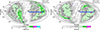 |
Fig. 9. Sky maps of S/N(Δℳ) and S/N(Δb). Dots represent the SNe in Pantheon+ (z < 1.121) and circles mark the maximum S/N values. |
To evaluate the probabilities of obtaining S/N(Δℳ)≥3.7 and S/N(Δb)≥3.3 by chance when scanning many directions on the sky (the look-elsewhere effect; Bayer & Seljak 2020), we performed 104 simulations. In each simulation, we randomised the RA and Dec coordinates of the SNe and produced the S/N(Δℳ) and S/N(Δb) maps using the HC method and the same directions as above. The probabilities of obtaining S/N(Δℳ)≥3.7 and S/N(Δb)≥3.3 by chance are 6.0% and 11.2%, respectively, corresponding to 1.9σ and 1.6σ significances. Therefore, we find no evidence for anisotropies in ℳ and b.
If the directions of maximum S/N(Δℳ) and S/N(Δb) were real anisotropies, detecting them at a 3σ level with the HC method would require adding 2500 and 4400 SNe to Pantheon+ (z < 1.121), respectively. An alternative approach would be to perform deep-field SN surveys towards the directions of the candidate anisotropies. This is particularly important given the absence of high-z SNe near those directions (see Fig. 9).
5.3. JWST, LSST, CSST, and Roman
Given the small number of SNe at z > 1.121, the validity of the empirical relation beyond this redshift remains to be verified. At present, the James Webb Space Telescope (JWST) is observing SNe Ia at z > 1.7 (Casey et al. 2023; DeCoursey et al. 2025). Siebert et al. (2025) report  for SN 2025ogs at z = 2.05, while Pierel et al. (2025) report
  for SN 2023aeax at z = 2.15 and
  for SN 2023adsy at z = 2.903. At these redshifts, adopting the parameters inferred from Pantheon+ (Table 2) and H0 = 70 km s−1 Mpc−1, the empirical relation predicts μ = 45.92, 46.04, and 46.71, whereas the ΛCDM model predicts μ = 46.0, 46.13, and 46.94, respectively. The μ values for SNe 2025ogs and 2023aeax are consistent with both relations, whereas that for SN 2023adsy is more consistent with the ΛCDM model than with the empirical relation. However, due to its red colour, it is uncertain whether SN 2023adsy is representative of high-z SNe Ia or an outlier (Pierel et al. 2024, 2025).
Beyond JWST, future deep-field surveys with the China Space Station Telescope (CSST; Li et al. 2023) and the Nancy Grace Roman Space Telescope (Hounsell et al. 2023) will observe SNe Ia up to z = 1.3 and z = 1.7, respectively. These SNe, combined with those observed by JWST and the 19 SNe at 1.121 < z ≤ 2.261 in Pantheon+, will be essential for determining the maximum z at which the empirical relation remains valid.
The deep rolling surveys of the Vera C. Rubin Observatory Legacy Survey of Space and Time (LSST; Gris et al. 2024) will provide photometry of thousands of SNe Ia with z ≲ 1.1. Thus, the Hubble diagram for each of the five LSST Deep Drilling Fields can be analysed with the empirical relation. Of these fields, the newly defined Euclid Deep Field South (RA = 61.241°, Dec = −48.423°), located at an angular separation of 21° from the S5 field, will enable study of cosmic acceleration in a direction distinct from those analysed here.
6. Conclusions
We present a new empirical m(z) relation based on data from Pantheon+ and DES-SN5YR. This relation fits their Hubble diagrams with only two parameters, ℳ and b, both of which can be computed analytically. Notably, under the FLRW metric, b ∝ q0 + 1.
For the DES-SN5YR and Pantheon+ Hubble diagrams, the empirical relation provides fits up to z = 1.121 that closely match those obtained with the Padé cosmography and the ΛCDM, flat ΛCDM, flat wCDM, and flat Padé models. The validity of the empirical relation beyond z = 1.121 cannot be reliably assessed given the small number of SNe at z > 1.121. Based on the ΔIC values, the empirical relation performs better than the ΛCDM model, the flat wCDM model, and the Padé cosmography, and comparably to the flat ΛCDM and flat Padé models.
For DES-SN5YR and Pantheon+ (z < 1.121), we obtain b = −0.628 ± 0.021 and b = −0.606 ± 0.026, respectively. We also applied the empirical relation to DES-Dovekie and Amalgame, obtaining b = −0.603 ± 0.020 and b = −0.613 ± 0.041, respectively. For Pantheon+ (z < 1.121) combined with SH0ES, we obtain H0 = 73.4 ± 1.0 km s−1 Mpc−1.
The empirical relation, as well as the flat ΛCDM and flat Padé models, remains stable in the absence of low-z SNe. Fitting the empirical relation to the Hubble diagrams of the eight deep-field regions, we find that their fitted ℳ and b parameters are consistent within 1.6σ, in agreement with isotropy. Applying an LRT, we find no evidence of anisotropy. This result is further supported by using the empirical relation in the HC method applied to Pantheon+ (z < 1.121), which finds no statistically significant evidence for anisotropies in ℳ and b.
Furthermore, the b values from the eight deep-field regions translate to q0 values ranging from −0.6 to −0.4, which are consistent within 1.6σ and lower than zero at 4.8σ. These results strongly support an accelerating universe, under the assumption that the large-scale density in each deep-field region is independent of the comoving radial coordinate.
Assuming an FLRW metric, the empirical relation can also be applied to BAO distances from DESI DR2, and to H(z) values from cosmic chronometers. The derived b values, assuming Ωk = 0, are largely consistent with those from DES-SN5YR, Pantheon+ (z < 1.121), DES-Dovekie, and Amalgame.
The empirical relation, m(z) =ℳ + bz + 5log(z(1 + z)), or equivalently  , provides a straightforward quantitative tool for fitting Hubble diagrams of SNe Ia without requiring a low-z sample. It enables tests of basic properties of the Universe in a simplified manner, reducing the computational cost typically associated with physically motivated cosmological models. Our analysis demonstrates that the empirical relation is valid at least up to z ≈ 1.1. Ongoing and upcoming deep SN surveys will allow us to test its validity at higher redshifts.
Acknowledgments
We acknowledge the Director of the Millennium Institute of Astrophysics (MAS), Francisco Förster, for financial assistance through ANID grant ICN12_009, and acknowledge complementary funding from ANID/FONDECYT grant 1251692. OR is supported by the Rubin-Chile Fund under grant DIA2650. We thank Felipe Asenjo and Ariel Órdenes for helpful discussions.
References
- Abdul Karim, M., Aguilar, J., Ahlen, S., et al. 2025, Phys. Rev. D, 112, 083515 [Google Scholar]
- Alfano, A. C., Cafaro, C., Capozziello, S., Luongo, O., & Muccino, M. 2026, J. High Energy Astrophys., 49, 100444 [Google Scholar]
- Baker, G. A., & Graves-Morris, P. 1996, Padé approximants (Cambridge, UK: Cambridge University Press) [Google Scholar]
- Bayer, A. E., & Seljak, U. 2020, JCAP, 2020, 009 [Google Scholar]
- Bochner, B., Pappas, D., & Dong, M. 2015, ApJ, 814, 7 [Google Scholar]
- Brout, D., Scolnic, D., Popovic, B., et al. 2022, ApJ, 938, 110 [NASA ADS] [CrossRef] [Google Scholar]
- Burnham, K. P., & Anderson, D. R. 2002, Model selection and multimodel inference: a practical information-theoretic approach (New York: Springer-Verlag) [Google Scholar]
- Camilleri, R., Davis, T. M., Vincenzi, M., et al. 2024, MNRAS, 533, 2615 [Google Scholar]
- Capozziello, S., D’Agostino, R., & Luongo, O. 2020, MNRAS, 494, 2576 [NASA ADS] [CrossRef] [Google Scholar]
- Casey, C. M., Kartaltepe, J. S., Drakos, N. E., et al. 2023, ApJ, 954, 31 [NASA ADS] [CrossRef] [Google Scholar]
- Cattoën, C., & Visser, M. 2007, Class. Quantum Gravity, 24, 5985 [Google Scholar]
- Clocchiatti, A., Rodríguez, Ó., Órdenes Morales, A., & Cuevas-Tapia, B. 2024, ApJ, 971, 19 [Google Scholar]
- Conley, A., Guy, J., Sullivan, M., et al. 2011, ApJS, 192, 1 [Google Scholar]
- DeCoursey, C., Egami, E., Pierel, J. D. R., et al. 2025, ApJ, 979, 250 [Google Scholar]
- Earp, S. W. F., Debattista, V. P., Macciò, A. V., et al. 2019, MNRAS, 488, 5728 [Google Scholar]
- Efstathiou, G. 2025, Philos. Trans. R. Soc. London Ser. A, 383, 20240022 [Google Scholar]
- Enqvist, K. 2008, Gen. Relativ. Gravit., 40, 451 [Google Scholar]
- Foreman-Mackey, D., Hogg, D. W., Lang, D., & Goodman, J. 2013, PASP, 125, 306 [Google Scholar]
- Gelman, A., & Rubin, D. B. 1992, Stat. Sci., 7, 457 [Google Scholar]
- Górski, K. M., Hivon, E., Banday, A. J., et al. 2005, ApJ, 622, 759 [Google Scholar]
- Gris, P., Awan, H., Becker, M. R., et al. 2024, ApJS, 275, 21 [Google Scholar]
- Hounsell, R., Scolnic, D., Brout, D., et al. 2023, ArXiv e-prints [arXiv:2307.02670] [Google Scholar]
- Hu, J. P., & Wang, F. Y. 2022, A&A, 661, A71 [NASA ADS] [CrossRef] [EDP Sciences] [Google Scholar]
- Hu, J. P., Hu, J., Jia, X. D., Gao, B. Q., & Wang, F. Y. 2024a, A&A, 689, A215 [NASA ADS] [CrossRef] [EDP Sciences] [Google Scholar]
- Hu, J. P., Wang, Y. Y., Hu, J., & Wang, F. Y. 2024b, A&A, 681, A88 [NASA ADS] [CrossRef] [EDP Sciences] [Google Scholar]
- Huang, L., Cai, R.-G., & Wang, S.-J. 2025, Sci. China Phys. Mech. Astron., 68, 100413 [Google Scholar]
- Kass, R. E., & Raftery, A. E. 1995, J. Am. Stat. Assoc., 90, 773 [Google Scholar]
- Koyama, K. 2016, Rep. Prog. Phys., 79, 046902 [NASA ADS] [CrossRef] [Google Scholar]
- Li, E.-K., Du, M., & Xu, L. 2020, MNRAS, 491, 4960 [NASA ADS] [CrossRef] [Google Scholar]
- Li, S.-Y., Li, Y.-L., Zhang, T., et al. 2023, Sci. China Phys. Mech. Astron., 66, 229511 [NASA ADS] [CrossRef] [Google Scholar]
- Linder, E. V. 2006, Phys. Rev. D, 74, 103518 [Google Scholar]
- Mc Conville, R., Colgáin, Ó. E., 2023, Phys. Rev. D, 108, 123533 [CrossRef] [Google Scholar]
- Odintsov, S. D., Sáez-Chillón Gómez, D., & Sharov, G. S. 2025, Eur. Phys. J. C, 85, 298 [Google Scholar]
- Perivolaropoulos, L., & Skara, F. 2022, New Astron. Rev., 95, 101659 [CrossRef] [Google Scholar]
- Perlmutter, S., Aldering, G., Goldhaber, G., et al. 1999, ApJ, 517, 565 [Google Scholar]
- Pierel, J. D. R., Engesser, M., Coulter, D. A., et al. 2024, ApJ, 971, L32 [Google Scholar]
- Pierel, J. D. R., Coulter, D. A., Siebert, M. R., et al. 2025, ApJ, 981, L9 [Google Scholar]
- Planck Collaboration VI. 2020, A&A, 641, A6 [NASA ADS] [CrossRef] [EDP Sciences] [Google Scholar]
- Popovic, B., Scolnic, D., Vincenzi, M., et al. 2024, MNRAS, 529, 2100 [CrossRef] [Google Scholar]
- Popovic, B., Shah, P., Kenworthy, W. D., et al. 2025, ArXiv e-prints [arXiv:2511.07517] [Google Scholar]
- Räsänen, S. 2006, JCAP, 2006, 003 [Google Scholar]
- Riess, A. G., Filippenko, A. V., Challis, P., et al. 1998, AJ, 116, 1009 [Google Scholar]
- Riess, A. G., Yuan, W., Macri, L. M., et al. 2022, ApJ, 934, L7 [NASA ADS] [CrossRef] [Google Scholar]
- Sako, M., Bassett, B., Connolly, B., et al. 2011, ApJ, 738, 162 [NASA ADS] [CrossRef] [Google Scholar]
- Sánchez, B. O., Brout, D., Vincenzi, M., et al. 2024, ApJ, 975, 5 [Google Scholar]
- Schwarz, G. 1978, Ann. Stat., 6, 461 [Google Scholar]
- Schwarz, D. J., & Weinhorst, B. 2007, A&A, 474, 717 [NASA ADS] [CrossRef] [EDP Sciences] [Google Scholar]
- Scolnic, D. M., Jones, D. O., Rest, A., et al. 2018, ApJ, 859, 101 [NASA ADS] [CrossRef] [Google Scholar]
- Siebert, M. R., Pierel, J. D. R., Engesser, M., et al. 2025, ArXiv e-prints [arXiv:2512.19783] [Google Scholar]
- Sugiura, N. 1978, Commun. Stat. Theory Methods, 7, 13 [Google Scholar]
- Vincenzi, M., Kessler, R., Shah, P., et al. 2025, MNRAS, 541, 2585 [Google Scholar]
- Weinberg, D. H., Mortonson, M. J., Eisenstein, D. J., et al. 2013, Phys. Rep., 530, 87 [Google Scholar]
- Wilks, S. S. 1938, Ann. Math. Stat., 9, 60 [Google Scholar]
- Wiltshire, D. L. 2009, Phys. Rev. D, 80, 123512 [Google Scholar]
- Zonca, A., Singer, L., Lenz, D., et al. 2019, J. Open Source Software, 4, 1298 [Google Scholar]
Data are available at https://github.com/CobayaSampler/bao_data/tree/master/desi_bao_dr2
All Tables
All Figures
|
Fig. 1. Sky distribution of Pantheon+ and DES-SN5YR SNe. Dashed lines indicate the Galactic equator. Plus and cross symbols mark the north and south Galactic poles, respectively. Circular and triangular regions are also shown. |
| In the text | |
|
Fig. 2. Relation between m − 5log(z(1 + z)) and z for Pantheon+ and DES-SN5YR. Binned data (blue squares) with error bars are shown for visualisation purposes only, both here and throughout the paper. |
| In the text | |
|
Fig. 3. Confidence contours at the 68.27% and 95.45% levels of the empirical relation parameters, obtained analytically and using EMCEE. |
| In the text | |
|
Fig. 4. Hubble diagrams of DES-SN5YR and Pantheon+, along with the best-fit m(z) relations. The lower panels show the residuals relative to the empirical relation. |
| In the text | |
|
Fig. 5. Distribution of q0 versus ℳ for the m(z) relations fitted to DES-SN5YR and Pantheon+ (z < 1.121) with different zmin. Solid curves are the 68.27% confidence contours for zmin = 0.01, while the contour of the empirical relation is shown as a shaded region in each panel for comparison. Although the flat wCDM constraints in the (w, ΩM) plane are highly non-Gaussian, their projection onto q0 leads to nearly symmetric uncertainties, as expected since q0 = QH(z = 0), where the parameter QH(z) is almost free of the w–ΩM degeneracy (Camilleri et al. 2024). |
| In the text | |
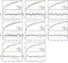 |
Fig. 6. Same as Fig. 4, but for the deep-field regions. |
| In the text | |
|
Fig. 7. Confidence contours (68.27%) and marginalised distributions of empirical relation parameters fitted to the deep-field regions. |
| In the text | |
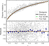 |
Fig. 8. Same as Fig. 4, but for the Amalgame SN sample. |
| In the text | |
|
Fig. 9. Sky maps of S/N(Δℳ) and S/N(Δb). Dots represent the SNe in Pantheon+ (z < 1.121) and circles mark the maximum S/N values. |
| In the text | |
Current usage metrics show cumulative count of Article Views (full-text article views including HTML views, PDF and ePub downloads, according to the available data) and Abstracts Views on Vision4Press platform.
Data correspond to usage on the plateform after 2015. The current usage metrics is available 48-96 hours after online publication and is updated daily on week days.
Initial download of the metrics may take a while.