| Issue |
A&A
Volume 709, May 2026
|
|
|---|---|---|
| Article Number | A135 | |
| Number of page(s) | 11 | |
| Section | Astrophysical processes | |
| DOI | https://doi.org/10.1051/0004-6361/202558669 | |
| Published online | 12 May 2026 | |
Timing analysis of the brightest X-ray flare of Sagittarius A* detected by XMM-Newton in 2019
1
Landessternwarte (LSW), Heidelberg University, Königstuhl 12, D-69117 Heidelberg, Germany
2
Max-Planck-Institut für Plasmaphysik (IPP), Boltzmannstraße 2, D-85748 Garching, Germany
3
Institute for Theoretical Physics, Heidelberg University, Philosophenweg 12, 69120 Heidelberg, Germany
4
Max-Planck-Institut für Kernphysik (MPIK), Saupfercheckweg 1, D-69117 Heidelberg, Germany
★ Corresponding author: This email address is being protected from spambots. You need JavaScript enabled to view it.
Received:
18
December
2025
Accepted:
19
February
2026
Abstract
Context. XMM-Newton has been monitoring Sgr A*, the supermassive black hole located at the dynamical centre of the Milky Way for more than two decades. A total of 91 observations were conducted from 1999 to 2023.
Aims. In this paper we focus on a time-binned analysis of 2019 observations with a time coverage of ≈460 ks to investigate the flaring activities of Sgr A*.
Methods. We proceeded background-subtracted light curves of the 2019 datasets for various on- and off-extraction regions to analyse the signal-to-noise ratio of the detected flares of Sgr A* and enhance the statistical significance of its variability in the X-ray band.
Results. Our results reveal that Sgr A* underwent six very bright flaring events during the 2019 XMM-Newton observations, from March to the end of September. We identified the five brightest flares of Sgr A*, observed over more than two decades (1999–2023), with two of these events occurring in 2019. Remarkably, Sgr A* exhibited its brightest flaring event reported so far on August 31, 2019 with a peak brightness and duration exceeding the previous four brightest flares by more than a factor of 2. This exceptionally bright flare, with a duration of 6.6 ks, featured an asymmetric energy-independent double-peak morphology. Spectral analysis of this double-peaked flare suggests spectral evolution during the event and highlights substructures on timescales as short as 100 s. We discuss the implications of the observed flaring activity for synchrotron and hotspot emission models.
Key words: acceleration of particles / accretion / accretion disks / astroparticle physics / magnetic fields / radiation mechanisms: non-thermal
© The Authors 2026
 Open Access article, published by EDP Sciences, under the terms of the Creative Commons Attribution License (https://creativecommons.org/licenses/by/4.0), which permits unrestricted use, distribution, and reproduction in any medium, provided the original work is properly cited.
This article is published in open access under the Subscribe to Open model. This email address is being protected from spambots. You need JavaScript enabled to view it. to support open access publication.
1. Introduction
Sgr A* is a variable, broadband source that emits light over a wide range of frequencies, from radio to X-rays (Macquart et al. 2006; Eckart et al. 2008; Yusef-Zadeh et al. 2009; Dodds-Eden et al. 2009). Sgr A* was first identified as a very compact, bright, and non-variable radio source at the dynamical centre of the Galaxy (Balick & Brown 1974). In its so-called ‘quiescent state’, most of the flux is emitted at sub-millimeter wavelengths through the synchrotron radiation of relativistic thermal electrons close to its supermassive black hole (BH) (Genzel et al. 2010). The faint and steady X-ray emission of Sgr A*, on the other hand, is believed to originate from thermal bremsstrahlung radiation within an optically thin, hot accretion flow (e.g., Baganoff et al. 2001, 2003; Yuan et al. 2003; Gillessen et al. 2017; GRAVITY Collaboration 2018a). Follow-up observations in multiple wavelengths, including in radio, near-infrared (NIR) and X-ray bands, have revealed Sgr A* variability. In the X-ray band, rapid variability in Sgr A* was first reported in 2001 based on Chandra observations (Baganoff et al. 2001). These observations showed that X-ray flares, which occur about once per day, can be ten times brighter than the quiescent background flux (Baganoff et al. 2001). Polarimetric observations of NIR flares, which occur more frequently – about 2−6 times per day (Genzel et al. 2003; Nishiyama et al. 2006) – suggest that a non-thermal synchrotron mechanism is responsible for the flaring activities in this band (Eckart et al. 2008). Simultaneous NIR and X-ray observations show that X-ray flares have NIR counterparts, whose light curves have similar shapes with no apparent delay (within 3 min) between the flare peaks (Yusef-Zadeh et al. 2006; Dodds-Eden et al. 2009; Eckart et al. 2012; Boyce et al. 2019, 2021).
Delayed sub-millimetre flares (e.g., approx. 100 min after the X-ray peak; Marrone et al. 2008), millimetre flares (up to 5 h; Yusef-Zadeh et al. 2006) and radio flares (ranging from hours to days; Yusef-Zadeh et al. 2017; Subroweit et al. 2017) have been interpreted as the result of the adiabatic cooling of an expanding relativistic plasma blob, with the observed emission primarily attributed to the synchrotron radiation from relativistic electrons. As the blob expands, adiabatic cooling reduces both the electron energies and magnetic field strength, leading to a decrease in the synchrotron self-absorption frequency and a shift in the emission towards longer wavelengths. Simultaneous variability in the NIR and X-ray bands suggests that the flares of Sgr A* in both wavelengths result from the same physical process and arise from a region close to the horizon of the BH (Eckart et al. 2004, 2008). Consequently, the X-ray variability of Sgr A* is also believed to be due to a broadband non-thermal emission. The observed emission can be interpreted within the framework of synchrotron or synchrotron self-Compton models (Dodds-Eden et al. 2009; Barrière et al. 2014; Eckart et al. 2012; Dibi et al. 2016) or inverse Compton models (Yusef-Zadeh et al. 2009; Dodds-Eden et al. 2009). In the latter, relativistic electrons emit synchrotron radiation in the NIR, while the inverse Compton scattering of synchrotron photons or soft photons from the accretion flow or stellar sources accounts for the observed X-ray flares.
While the mentioned radiation mechanisms describe how relativistic particles emit photons in the NIR and X-ray bands, the physical processes responsible for accelerating these particles remain uncertain. Several scenarios have been discussed, including magnetic reconnection (e.g., Dexter et al. 2020; Ripperda et al. 2020; Porth et al. 2021), accretion instabilities (e.g., Tagger & Melia 2006), and shocks within the accretion flow (e.g., Mandal & Chakrabarti 2005).
Additionally, hotspot models, in which localized regions of plasma orbit near the event horizon, have been proposed as a mechanism to explain the bright variability observed in the light curves of Sgr A*. The emission from these hotspots is influenced by relativistic effects such as Doppler boosting, gravitational redshift, and gravitational lensing (e.g., Meyer et al. 2006; Trippe et al. 2007; Genzel et al. 2003; Broderick & Loeb 2005; Hamaus et al. 2009). Hotspot models suggest that a combination of these effects can account for the characteristic double-peak light curves observed during some of Sgr A*’s flares (Mossoux et al. 2016; Karssen et al. 2017), with one peak attributed to gravitational lensing as the hot spot passes behind the BH and the other due to Doppler boosting as it moves towards the observer. Additionally, light-travel time delays caused by variations in the photon path lengths around the BH can introduce asymmetries in the timing and shape of the observed flare profile. For example, Karssen et al. (2017) show that the asymmetric light curves of the bright Sgr A* flares (Baganoff et al. 2001; Porquet et al. 2003, 2008; Nowak et al. 2012) could be accounted for by luminous hotspots orbiting at approximately 10 − 20 gravitational radii (rg, see also von Fellenberg et al. 2023, 2024). Such orbital scales are commonly invoked in hotspot models (e.g., Genzel et al. 2003; Hamaus et al. 2009; GRAVITY Collaboration 2018b). Challenges remain, however, for flares that show a large flux decay between the two peaks (Mossoux et al. 2016). This suggests that additional effects such as interactions with the underlying accretion flow or multi-zone emission regions, may need to be considered. Finally, external processes, such as the interaction between orbiting stars and the hot accretion flow (Nayakshin et al. 2004), the tidal disruption of asteroids (Zubovas et al. 2012; Seoane 2025), or increases in the accretion rate due to fresh material reaching the BH (Czerny et al. 2013), have also been proposed. We note that interpretations can be complicated by the fact that the nature of the flares, at least in the NIR, is not always clear (e.g., Do et al. 2009; Meyer et al. 2014; Witzel et al. 2018).
Time-resolved spectral analysis can, in principle, help in distinguishing between competing physical models and can provide insights into the underlying particle acceleration and emission mechanisms. Ponti et al. (2017), for example, show that the combined NIR–X-ray spectra of bright flares from Sgr A* can be described by a synchrotron cooling-break model with a slowly evolving high-energy cutoff. For the bright NIR and moderate X-ray flare of Sgr A* from July 2019, GRAVITY Collaboration (2021) find that the mean spectral energy distribution can be successfully reproduced by a synchrotron model with a cooling break plus an exponential high-energy cutoff. More recently, James Webb Space Telescope (JWST) Near Infrared Camera (NIRCam) and Mid-Infrared Instrument (MIRI) observations have revealed that the spectral index depends on flare flux density, which is indicative of synchrotron cooling shaping the observed spectrum (e.g., Yusef-Zadeh et al. 2025; von Fellenberg et al. 2025). These results illustrate the importance of multi-wavelength studies for understanding flare physics.
In this paper, in a continuation of the dataset analysis of the XMM-Newton observations from 1999 to 2018 (Ponti et al. 2015; Mossoux & Grosso 2017; Mossoux et al. 2020), we focus on XMM-Newton observations of Sgr A* from 2019 to 2023, reporting the brightest flare detected by XMM-Newton, which occurred on August 31, 2019. The brightest X-ray flare of Sgr A* reported so far, with a peak amplitude of ≈1.74 (cts/s) and a duration of ≈2.7 ks, was detected by XMM-Newton, on October 3, 2002 (Porquet et al. 2003). This flare was found to have an almost symmetrical light curve with respect to the flare peak with no significant difference between the soft and hard X-ray range. Porquet et al. (2008) and Dodds-Eden et al. (2009) later reported a flare that occurred on April 4, 2007, the (then) second brightest X-ray flare of Sgr A*, it had a peak amplitude of ≈1.05 (cts/s) and was followed by three flares of more moderate amplitudes. This light-curve shape (nearly symmetrical), duration (≈3 ks) and spectral characteristics of the flare were similar to the very bright flare observed in October 3, 2002. Within the XMM-Newton observational dataset up to 2015, a flare detected on August 30, 2014 was subsequently found to be brighter than the one observed on April 4, 2007 (Ponti et al. 2015; Mossoux & Grosso 2017). Ponti et al. (2017) describe the 2014 August 30−31 (VB3) flare as a bright, initially NIR-dominated event with a delayed and spectrally evolving X-ray component. The X-ray flare, with a total duration of approximately 3 − 4 ks, reached a peak 2−10 keV luminosity of LX ≃ 4 × 1035 erg s−1.
In the following, we focus on the analysis of the brightest flaring activity of Sgr A*, detected on August 31, 2019. Section 2 presents the list of all 2019 XMM-Newton observations, followed by a description of the data reduction process. Section 3 shows the light curves from all 22 XMM-Newton observations of Sgr A* in 2019. Section 4 reports the results of the timing analysis of the August 31, 2019, flare. In Section 5, we discuss implications for hotspot models and provide our conclusions in Section 6.
2. Observations and data reduction
Focusing on the flare year, Table A.1 Appendix A lists all XMM-Newton observations of Sgr A* in 2019, with a total time duration of ≈460 ks between March and September. For data reduction and analysis, we followed the standard XMM-Newton procedures using the Science Analysis Software (SAS), version 20.0.0, together with the corresponding current calibration files.
To look for the variability of the XMM-Newton observations, using the task evselect, we extracted the events of the source + background region from an aperture of 10″ (or 200 in sky coordinate units of 0.05 arcsec/pixel) centred on the very long-baseline interferometery radio position of Sgr A*: RA(J2000) =  , Dec(J2000) =
  (Reid et al. 1999). The contribution of the background events was estimated from an annulus extraction region far away from the source with inner and outer radius size of 175″ and 200″ (or 3500 and 4000 in sky coordinates units of 0.05 arcsec/pixel). For the purpose of single to noise ration (S/N) studies, we also defined three other circular on-regions with radii of 12.5″, 15″ and 17.5″ (or 200, 250, 300 and 350 pixels in sky coordinate with 0.05 arcsec/pixel resolution) and also a 1.5′×1.5′ (or 1800 × 1800 in sky coordinate units of 0.05 arcsec/pixel) box background region at ≈4′ north of Sgr A*, where the X-ray emission is low (minimum X-ray diffuse emission and absence of bright X-ray sources).
The light curves of the source + background and background regions were created from single, double, triple, and quadruple events (PATTERN ≤ 12) for both the MOS1 and MOS2 cameras and from single and double events (PATTERN ≤ 4) for the PN camera. For the PN camera we also used FLAG= = 0 to reject the dead columns and bad pixels. Since photon pile-up can affect the relative fractions of single and multiple event patterns (cf. Jethwa et al. 2015), we checked for pile-up using the SAS task epatplot, which compares the observed event pattern fractions with the expected instrumental model. The analysis was performed for the European Photon Imaging Camera PN, MOS1, and MOS2 cameras using the same source extraction region as in the timing and spectral analysis. No significant excess of higher-order event patterns was found, and the observed single- and double-event pattern fractions are consistent with the expected distributions within the uncertainties. We therefore conclude that pile-up does not affect the data significantly, and no core excision or pile-up correction is required. Light curves were computed in the 2−10 keV energy range using time bins of 300 s and 100 s. In the end, the task epiclccorr applies time-dependent and energy-dependent corrections to the light curves and produces the background-subtracted light curves. We then summed the background-subtracted light curves of the three cameras to produce the summed EPIC light curves. For our time series analysis, we did not clean the calibrated event list for soft proton contamination or background flaring activities, as our focus was on the flux variability (photon counts) in the source light curves, with the background already subtracted. We also did not mask other X-ray sources within the 10″ source aperture during our timing analysis, since the flaring emission from Sgr A* dominates and the potential contamination is minimal.
3. Timing analysis
We derive source background-subtracted light curves (counts vs time) of all 2019 observations listed in Table A.1 Appendix A in the 2−10 keV energy range, for the circular source extraction region of 10″ and for a time bin-size of 300 s. The background events of each case are estimated from an annulus extraction region far away from the source, with inner and outer radius size of 175″ and 200″. The background counts are subsequently normalized to the source extraction region. For observation 0851181001, Sgr A* is out of the field of view, resulting in 21 light curves.
3.1. Flare identification
To identify X-ray flares from Sgr A*, Ponti et al. (2015, 2017) and Mossoux et al. (2015, 2016) applied the Bayesian blocks algorithm to unbinned photon arrival times, defining flares as statistically significant deviations from the quiescent emission level within a Poisson likelihood framework. In Mossoux et al. (2015, 2016), the method was further refined through a two-step procedure that accounts for background variability and controls the false-positive rate via Monte Carlo simulations. While Bayesian blocks methods are optimal for flare detection in the low-count regime, time-binned analyses provide a robust and homogeneous framework for variability studies across large samples of observations. Therefore, in this work, we adopted a time-binned approach, a method commonly employed in previous studies (Porquet et al. 2003, 2008), to characterize the variability of Sgr A* across the 21 observations. We identified epochs in which the flux is significantly higher than the non-flaring (quiescent) level. The average flux value for each observation, defined as the total number of counts divided by the number of time bins within the on-source aperture, is listed in Table A.1 Appendix A. We classified observations with identical average fluxes (within the noise) as observations with no variability and those with average fluxes outlying the rest (or non-flaring flux of Sgr A*) as observations with variability. Based on this definition, out of a total of ≈452 ks of XMM-Newton observations in 2019, six observations reveal bright/very bright and single/multiple flaring activities above 3σ significance: March 11 (Obs.ID 0831800101), March 14 (Obs.ID 0831800401), March 16 (Obs.ID 0831800601), March 30 (Obs.ID 0822680301), April 3 (Obs.ID 0831801001) and August 31 (Obs.ID 0831801201). Note that in observations marked as with no variability based on their averages fluxes, the corresponding rms values are also consistent (within the noise level).
Figure A.1, Appendix A shows the light curves of these six flares. As can be seen, the flare observed on August 31 (Obs.ID 0831801201) stands out prominently and is the primary focus of this paper. Note that events are detected primarily by the PN camera due to its higher effective area (Ponti et al. 2015). The effective areas of the two MOS cameras are lower than that of the PN, because only part of the incoming radiation falls onto these detectors.
For two reasons we performed aperture photometry analysis while studying the variability of a Sgr A*: One reason was to check if a flare does not come from Sgr A* but from a region that is very close to it, on the scale of point spread function. Source background-subtracted light curves of the observations with flare, within different on-region apertures of 10″, 12.5″, 15″ and 17.5″ all co-centric on the position of Sgr A*, show a consistency in growth of the signal by going to the larger apertures, indicating that the observed variations are most likely coming from the Sgr A* and not from another X-ray source in its vicinity. The second reason was to find the optimal choice of on-region aperture in terms of the S/N. In general, for very bright flares, it is preferable to use a smaller aperture to minimize background noise by limiting the number of included pixels. Conversely, for rather faint flares, a larger aperture may be more appropriate in order to capture as much of the flare signal as possible, despite the increased background contribution. Therefore, the optimal choice of the aperture size is determined following the maximum S/N. In our studies, we choose an aperture that encompasses both high- and low-flux flares homogeneously. By examining how the quiescent (non-flaring) flux and the flare flux – after quiescent subtraction – vary with aperture size, we were able to determine the most suitable aperture for our study. Our analysis shows, for example, that for the moderately bright flare of Sgr A* on August 14 (observation 0831800401) increasing the aperture radius from 10″ to 17.5″ results in no significant change in the measured flare flux within the noise level. Therefore, we conclude that a 10″ radius is already a suitable choice for the on-source region in our study. We also explored two different background extraction regions, one using a 1.5′×1.5′ box region approximately 4′ north of Sgr A*, and an annulus background extraction region with inner and outer radius size of 175″ and 200″, respectively, for our subsequent analysis (Fig. 1).
 |
Fig. 1. Sky image of Sgr A* from the XMM-Newton observation on August 31, 2019. The source extraction region is a circular aperture of radius 10″ centred on the very long-based interferometry radio position of Sgr A*. The background is extracted from an annulus with inner and outer radii of 175″ and 200″, respectively. |
We note that in all six observations with variability, the background light curve is flat within statistical fluctuations. For instance, the light curve of April 3 (Obs.ID 0831801001) in (Fig. A.1, Appendix A) shows no background flaring that could affect the detector. Background subtraction was nonetheless performed to remove any such contributions, ensuring that the reported flares are intrinsic to the source. This is expected, as the background region, an annulus placed far from Sgr A* minimizes source contamination.
3.2. Flaring activity of August 31 observation
Of the six mentioned observations in 2019 that exhibited variability, those on March 16 (Obs.ID 0831800601) and August 31 (Obs.ID 0831801201) showed the highest brightness. In this paper, we focus on the flaring activity on August 31. We sum up source background-subtracted light curves of the three XMM-Newton cameras (MOS1, MOS2, and PN) in the 2−10 keV energy range for time bin sizes of 300 s and 100 s, respectively. We summed up the counts detected by all cameras to benefit from both the better spatial and angular resolution of the MOS cameras, which allow for more detailed imaging of sources due to their smaller pixel sizes, and the higher sensitivity and temporal resolution of the PN camera, which has a larger detector area, making it more effective for time-resolved observations. The PN camera also offers a faster time resolution of 0.03 ms compared to the 1.75 ms of the MOS cameras.
4. Results
4.1. The brightest flare of Sgr A*
Analysis of X-ray observations from 1999 to 2018 (Mossoux & Grosso 2017; Mossoux et al. 2020), identified 19 flares detected with XMM-Newton. Among these, the flares on October 3, 2002 (Obs.ID 0111350301), April 4, 2007 (Obs.ID 04024300401) and August 30, 2014 (Obs.ID 0743630201) are the brightest. The flares on October 3, 2002, and April 4, 2007, were initially reported as the first and second brightest flares of Sgr A* (Porquet et al. 2003, 2008). However, the flare on August 30, 2014, was later found to be brighter than the one on April 4, 2007. As we show here, Sgr A* has not only experienced significant flaring activity on March 16, 2019, and August 31, 2019, but the one on August 31, 2019 is in fact the brightest detected among all the other flares reported so far. Fig. 2 illustrates the light curves of the five brightest flares of Sgr A* detected by XMM-Newton from 1999 to 2019. The characteristic of these very bright flares based on only PN camera events, for bin size of 300 s are listed in Table 2.
 |
Fig. 2. Background-subtracted 2−10 keV PN light curves (300 s bins) of the five brightest X-ray flares detected from Sgr A*. The August 31, 2019 flare (Obs.ID 0831801201) is shown together with bright flares observed in 2002 (0111350301), 2007 (0402430401), 2014 (0743630201), and on March 16, 2019 (0831800601). Source counts are extracted from a circular region of radius 10″, and the background from an annulus with inner and outer radii of 175″ and 200″. Time zero corresponds to the start of each observation (see Table A.1). |
For each flare, the peak count rate or flux corresponds to the bin with the highest counts per unit time. Consequently, the derived peak count rate depends on the chosen bin size, in our case 300 s. This implies that if the bin size is changed, the peak count rate will vary accordingly. Smaller bin sizes can provide a more detailed view of rapid changes in flux, whereas larger bin sizes could smooth out variations and reduce the apparent peak value. To calculate the pre- and post-flare fluxes, we added up the counts of all bins that are consistent and close to an average value, and then divided this sum by the duration of all corresponding bins. To estimate the duration of a flare, we identified the first bin where the count rate is higher than the average or pre- and post-flare flux, and set the start time of this bin as the beginning of the flare; similarly, we identify the last bin where the count rate is still higher than the average and set the end time of this bin as the end of the flare.
To enable further comparison, we extended the data analysis to incorporate XMM-Newton observations from 2020 to 2023, These reveal two further bright flares, one on September 14, 2020, and one on March 26, 2022 (Fig. A.2, Appendix A). The derived characteristics of these two flares indicate that the events shown in Fig. 2 still represent the top five brightest flares detected by XMM-Newton from 1999 to 2023 and among them, the flare observed on August 31, 2019, remains the brightest X-ray flare from Sgr A* detected by XMM-Newton up to 2023.
To estimate the flare luminosity, we used the Portable, Interactive Multi-Mission Simulator (PIMMS), adopting parameters consistent with previous work. In particular, we assumed a power-law spectrum with photon index Γ = 3 and an interstellar hydrogen column density NH = 3.4 × 1023 cm−2, following Porquet et al. (2003), and used the EPIC PN medium filter response in the 2−10 keV band. These values lie within the range typically reported in subsequent X-ray studies of Sgr A* flares, which find photon indices Γ ∼ 2 − 3.5, depending on flare brightness, energy coverage and absorption. This approach yields an order-of-magnitude estimate of the mean intrinsic luminosity and allows direct comparison with earlier flare measurements. Accordingly, the August 2019 flare is characterized by a mean (intrinsic) luminosity of Lint ≃ 6 × 1035 erg/s. Note that flare identification here is defined in terms of peak count rate, reflecting the fact that our analysis is based on light curves and relative photon count variability without time-resolved spectral fitting; consequently, direct comparisons with flares characterized by unabsorbed luminosities from spectral modelling (e.g., Chandra’s brightest flare reported by Haggard et al. 2019) should be treated with some caution.
4.2. Double-peak morphology
If we sum up the events in the 2−10 keV energy range from August 31, 2019, detected by both the MOS and PN cameras, and plot the resultant (counts vs time) light curve for time bin sizes of 300 s and 100 s (Fig. 3), we see that Sgr A*’s brightest flare has a double-peak structure with an asymmetric morphology: a combination of two separate peaks, with a time delay between them. The histogram light curve of this observation, with 100 s time bin size shows this double-peak morphology more clearly. As can be seen, background counts (corrected for time-dependent inefficiencies and normalized to the source extraction region) are negligible compare to the source counts in this observation. Soft proton flaring counts of the full detector light curve in the 2−10 keV energy range are comparatively high only in the beginning and the end of the observation, where Sgr A* is not experiencing any flaring activity. These effects are not a concern, however, as all background counts, including those associated with flaring, are in the end subtracted from the source. To investigate whether the double-peak feature is energy-dependent, we divided the X-ray emission into two energy bands, soft (2−5 keV) and hard (5−10 keV). As shown in Fig. 4, after overlaying the soft- and hard-band light curves and subtracting the steady X-ray emission from each band, the double-peak morphology of the August 31, 2019, flaring activity appears consistent across energy bands. Since the 2−10 keV energy range is common to all cameras, we do not expect any significant changes arising due to the different spectral responses of the XMM-Newton instruments. We note that the light curve is restricted to the interval corresponding to the flaring activity, from 5400 s to 12 000 s, using a time binning of 100 s (i.e., a total duration of 6600 s) and is subtracted from the steady X-ray emission.
 |
Fig. 3. Summed background-subtracted 2−10 keV light curves detected by MOS1, MOS2, and PN for time bins of 300 s (left) and 100 s (right), within the common exposure time, for the August 31, 2019, observation (Obs.ID 0831801201). |
4.3. Spectral behaviour
As shown in Fig. 4, during the second peak of the August 31, 2019, flare, there appears to be an additional sub double-feature in the hard band (5−10 keV) that is not present in the soft band. In particular, a narrow pronounced feature emerges at the onset of the hard band, with no corresponding feature in the soft band. On the other hand, another narrow feature is observed at the end of the soft band (2−5 keV), accompanied by a much weaker counterpart in the hard band. These findings may indicate notable spectral variability during the second peak (feature) of the flare. In general, the overall fall or decay times of the light curves in the two bands are comparable, consistent with a flare governed by geometrical effects.
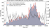 |
Fig. 4. Combined background-subtracted 2−10 keV light curves detected by MOS1, MOS2, and PN during the flaring activity of the August 31, 2019, observation (5400−12 000 s). The soft (2−5 keV) and hard (5−10 keV) bands are shown, and the hardness ratio (hard/soft) is overplotted (see the right-hand axis). The temporal evolution of the hardness ratio indicates spectral variability during the flare. |
As a first step in exploring the nature of the narrow features observed during the second peak of the August 31, 2019, flare, we evaluated the uncertainties in the total counts per bin. We used the uncorrected (source-plus-background) count data at this step, avoiding normalization or corrections affecting the raw statistical behaviour of the data. Analysis of the uncertainties (error bars) of the uncorrected source-plus-background counts as a function of time (Fig. A.3 Appendix A) reveals no strong short-term variations, with deviations remaining below the 2σ level. However, error bars alone are insufficient to fully assess the significance of possible short-timescale fluctuations. This motivates the use of additional significance tests that explicitly account for counting statistics and bin-to-bin variations (see Sect. 4.4).
To quantify the spectral evolution during the flare, we computed the hardness ratio and plotted it with the corresponding uncertainties. Based on the hardness ratio values and their associated errors in each time bin, we find indications for spectral evolution during the flare (Fig. 4). For comparison, previous Chandra studies of bright Sgr A* flares have not reported significant spectral evolution. Haggard et al. (2019) analysed the two brightest Chandra X-ray flares detected on September 14, 2013, and October 20, 2014. The 2013 flare, the brightest on record, lasted 5.7 ks and exhibited a double-peaked morphology, with peak count rates of 1.04 ± 0.06 and 0.93 ± 0.06 (cts/s). The 2014 flare, about 2.5 times less luminous, lasted 3.4 ks and showed an asymmetric morphology similar to the bright February 9, 2012, flare. The hardness ratios and spectral indices were found to remain constant throughout these flares. Similarly, Nowak et al. (2012) reported no spectral evolution during the bright flare on February 9, 2012, flare (duration of 5.6 ks), which was comparable in magnitude but longer in duration than the bright XMM-Newton flare observed in October 2002 (Obs.ID 0111350301 from Table 1). According to Porquet et al. (2003), no significant spectral evolution is observed between the 2−5 keV and 5−10 keV ranges for the October 2002 flare. These results may indicate a particular complexity in the August 31, 2019, flare.
Characteristics of the five brightest Sgr A* flares detected by XMM-Newton (PN camera).
4.4. Substructures
The narrow features observed at the beginning and end of the second peak of the August 31, 2019 flare could indicate the presence of substructures in both hard and soft bands. Fast variability may suggest that the flaring activity involves compact sub-regions within the emitting region. Temporal substructures within X-ray flares, on timescales shorter than 300 s, have been frequently reported (Baganoff et al. 2001, 2003; Porquet et al. 2003, 2008; Eckart et al. 2004; Nowak et al. 2012; Neilsen et al. 2013, 2015). According to Porquet et al. (2003), the 2002 flare (Obs.ID 0111350301 from Table 1) exhibits a substructure at about 11 200 s in both bands, with a significance of at least 3σ on a timescale as short as 200 s. For the February 9, 2012 X-ray flare observed by Chandra, Nowak et al. (2012) also report evidence of substructure based on a Bayesian blocks decomposition, with the flare peak being consistent with having a ≈300 s dip between two sharp peaks of ≈100 s duration. This substructure is similar to the one observed during the 2002 October flare detected by XMM-Newton.
Qualitatively, the hard (5−10 keV) X-ray light curve for the August 31, 2019 observation with 100 s binning reported here (Fig. 1), exhibits a behaviour (rise and decay) reminiscent of the flare observed in 2002 (Porquet et al. 2003). We note that for the 2019 flare, the fast variability remains resolved and is not washed out when the resolution is reduced from 50 to 100 s (see Fig. A.4 in Appendix A), while it is washed out going to a bin size of 200 s. This suggests a potential micro-structure during the second peak, on a timescale as short as 100 s. To explore this in more detail, we employed different significance tests (e.g., see Fig. 5). The per-bin significance compared to the baseline shows clear excesses in all cameras, across both the soft and hard energy bands, and for both 50 s and 100 s binning. For the two narrow peaks of interest (the hard substructure at t ∼ 9600 s and the soft substructure at t ∼ 10 900 s), both per-bin and integrated tests give strong results (5 − 7σ). Both substructures exhibit a strong bin-to-bin increase, with the 9600 s feature being particularly sharp. The fact that the narrow peaks persist across bins, appear in all EPIC cameras, and are seen in both soft and hard bands supports that they are real astrophysical signals and not statistical noise.
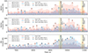 |
Fig. 5. Background-subtracted light curves of Sgr A* for the August 31, 2019, observation (Obs.ID 0831801201), shown separately for MOS1, MOS2, and PN. Counts per bin are plotted for the soft (2−5 keV) and hard (5−10 keV) bands using 50 s and 100 s binning. Horizontal dashed lines indicate baseline levels, while dotted and dash-dotted lines show the 3σ and 5σ thresholds. Shaded regions highlight narrow substructures near 9600 s (hard band) and 10 900 s (soft band), with their central times marked by vertical lines. Bins with jump significances exceeding 3σ are indicated. |
For the first peak of the August 31, 2019, flare, we also observe hints of substructure. These features reach per-bin significances above 5σ, in some cases, but their significance does not remain consistent across different bin sizes and instruments. In particular, they become weaker when using 50 s bins and do not show the same persistent behaviour as the substructures in the second peak. We therefore regard the evidence for substructure in the first peak as inconclusive.
5. Implications for hotspot models
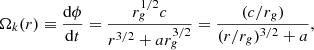
As shown above, the light curve from August 31, 2019 exhibits an asymmetric, double-peak morphology, resembling modulations associated with relativistic effects from a compact hotspot orbiting Sgr A* (e.g., Mossoux et al. 2016; Karssen et al. 2017). A potential constraint on micro-variability on a timescale tv will constrain the size of the emitting region (e.g., the hotspot; neglecting Doppler modifications) to Δr ≤ ctv. The evidence that tv ∼ 100 s during the second peak thus implies Δr ≲ 5rg, where rg = GM/c2 = 6.4 × 10¹¹(MBH/4.3 × 106 M⊙) cm is the characteristic gravitational radius for the BH mass of Sgr A* (e.g., GRAVITY Collaboration 2023). To explore this possibility further, we described the data by fitting a simple model with two Gaussians plus a constant baseline (Fig. 6). This fit reproduces the timing and relative amplitudes of the two maxima, though with a relatively high reduced chi-square, χν2 = 4.45, indicating that substructures are not fully captured. Adding an additional component (three-Gaussian fit), the reduced chi-square value improves to 3.68. However, its overall contribution to the flux remains small. Morphologically, the first component (Gaussian 1) is broader and lower, whereas the second (Gaussian 2) is narrower and taller. Near the second peak, the data rise more slowly than the symmetric profile predicts and decay more slowly afterwards, suggesting a slight asymmetry. The inferred separation of the two maxima is Δt = 2075 ± 124 s and the respective rise times are τe, 1 ≃ 1366 s and τe, 2 ≃ 608 s. The first (Gaussian) peak rises above the non-flaring, baseline level (N ≃ 40) by a factor of f1 ≃ 7, and the second (Gaussian) peak by a factor of f2 ≃ 15.
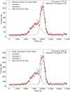 |
Fig. 6. Double-Gaussian (top) and three-Gaussian (bottom) fits to the summed light curve (counts vs time) of the August 31, 2019, Sgr A* flare. Time zero corresponds to the start of the observation (Table A.1). |
Hotspot models are often agnostic to plasma physical details (e.g., the specifics of the underlying acceleration mechanisms) and typically consider a compact, homogeneously emitting, spherical component (‘blob’), orbiting in a semi-equatorial plane at radius r with relativistic Keplerian angular velocity
 (1)
(1)
where a is the dimensionless BH spin parameter (a = 0 for a Schwarzschild BH) and prograde motion has been assumed. For a quasi-steady emitter, magnification effects can arise from a combination of relativistic Doppler boosting and gravitational lensing. Both are inclination-dependent, and reach their minimum for face-on orbits (i = 0°). As the inclination angle increases, the strength of both effects grows, albeit at different rates. For inclination angles i < 30°, gravitational lensing remains negligible for a compact hotspot, but becomes significant for i > 50° (e.g., Broderick & Loeb 2005; Hamaus et al. 2009; Karssen et al. 2017). The lensing peak is typically narrower, but can be broadened and partially or fully swamped by the Doppler contribution, depending on blob size Δr and location r. Gravitational lensing is strongest when the blob passes directly behind the BH. For inclinations of i ∼ 90° (edge-on), lensing alone can lead to flux magnifications by a factor of ∼10 − 20, roughly scaling with distance as r1/2. Doppler amplification of the flux, which approximately scales with D4, exhibits an opposite radial dependence. In the special relativistic regime, the Doppler factor is given by
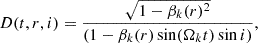 (2)
(2)
where βk(r) = Ωk(r)r/c. Since βk(r) decreases with increasing radius, D correspondingly decreases with r (as well as with decreasing inclination angle i). The innermost stable circular orbit for an accretion disk around a Schwarzschild BH lies at r = 6rg, while it can approach r = rg in the Kerr BH (a = 1) case. Hence, the Doppler factor is unlikely to exceed Dmax ≃ 1.8, implying that the maximum amplification in the absence of a baseline (disk background) emission is limited to (Dmax/Dmin)4 ∼ 40. Variations are possible if the hotspot moves very close to the innermost stable circular orbit in the Kerr BH case, where general relativistic (geodesic) effects become important. On the other hand, in the presence of a disk background, the observed amplification is likely to be reduced. In any case, interpreting the observed light curve of the August 31, 2019 flaring event in terms of a single hotspot requires a substantial orbital inclination. For example, at i ≤ 50°, Dmax/Dmin ≲ 1.8 for orbital motion at r ≥ 6rg around a Schwarzschild BH, resulting in modest Doppler amplification only. In the absence of some orbital precession over time or flaring-induced tilting of the hotspot’s orbit, higher inclinations would seem to be in tension with estimates of other hotspots’ motion around Sgr A* inferred from NIR observations (e.g., GRAVITY Collaboration 2018b, 2023; von Fellenberg et al. 2024). It remains to be explored to what extent a non-isotropically emitting source could help alleviate this.
In hotspot models, the phase lag f ≡ Δt/P between the beaming and lensing maxima usually decreases mildly as inclination increases. If the second peak were assumed to be lensing-related, for example, the beaming–lensing phase difference for a compact blob at high inclinations (i ∼ 90°) is approximately Δt ≃ 3P/4. Using our measured Δt, this would imply
 (3)
(3)
While this would be remarkably close to the orbital period (P ≃ 40 ± 15 min) inferred for NIR hotspot motion in 2018 (GRAVITY Collaboration 2018b) and to the transient (∼36 min) periodicity in the mid-infrared (Spitzer) light curve in July 2019 (Michail et al. 2024), it would not be compatible with the observed duration of the flaring activity in August 2019.
Alternatively, if the second peak were assumed to be Doppler-related instead, the phase difference at high inclination is approximately Δt ≃ P/4, translating into
 (4)
(4)
For a circular orbit in Schwarzschild space-time, this would correspond to a characteristic orbital radius of
 (5)
(5)
with orbital speed v/c ≃ 0.25. At these distances, however, Dmax ≲ 1.3, which makes it challenging to account for Doppler amplifications by a factor of ∼15, unless the blob is extended (Δr > rg, allowing for orbital superposition) and/or undergoes internal X-ray brightening within ≲P/4. The latter remains possible and may arise, for instance, if the injection rate of particles undergoing acceleration increases, or if the local field becomes amplified. On the other hand, if the flaring activity is dominated solely by a compact (quasi-steady) blob with Doppler factor D(t), the rise and decline time will in principle also depend on location, i.e., roughly as 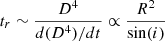 . With our measured τe, 2 this would rather be suggestive of orbital distances
 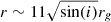 . In addition, the broadness of the first peak would seem challenging to account for with gravitational lensing. While the second scenario may seem slightly preferred, we note that a significant inclination would still be required. We caution, however, that detailed ray-tracing and dynamical flux-evolution modelling are required to assess whether the light curve can be reproduced with a single hotspot.
As noted in Sect. 4.1, the inferred mean intrinsic luminosity of the August 2019 flare is of order Lint ≃ 6 × 1035 erg/s. This can be compared with an X-ray synchrotron interpretation. Assuming a compact emitting region (a ‘blob’) of characteristic size rb and luminosity Lb = 1035l35 erg/s, the corresponding photon energy density is uph ≃ Lb/(4πrb2c) = 0.65l35(rg/rb)2 erg/cm3. If the X-rays are produced via non-thermal synchrotron emission, then relativistic electrons with Lorentz factors γe ∼ 106 (B/1 G)−1/2 are required to emit synchrotron photons at ∼5 keV (neglecting Doppler boosting). These high-energy electrons undergo synchrotron cooling on a cooling timescale ts ∼ 25 (B/10 G)−3/2 s, corresponding to a cooling length lc = cts, which is comparable to the gravitational scale rg. Hence, an efficient re-acceleration mechanism, such as reconnection and/or stochastic acceleration, would be needed in order to sustain the flare over its observed duration. Since synchrotron cooling is energy-dependent (tS ∝ 1/γ), lower-energy emission can exhibit longer characteristic timescales. It may be interesting to compare this with recent JWST observations of hour-type flaring activity, which revealed variability and wavelength-dependent time delays indicative of spectral evolution, on timescales as short as ∼10 minutes in the near-and mid-infrared (e.g., Yusef-Zadeh et al. 2025; von Fellenberg et al. 2025). In the synchrotron scenario, the total energy content of the radiating electrons, with number Ne, approximately satisfies NeEe ∼ Lsts with Ls = Lb. Requiring that the non-thermal electrons remain magnetically confined, uB := (B2/8π)≳ue ≃ NeEe/(4πrb3/3), then implies  G. For comparison, the characteristic maximum magnetic field on BH horizon scales (∼rg) is of order BH ∼ 100 G (e.g., Katsoulakos et al. 2020), and for an advocation-dominated accretion flow-type disk approximately scales with B(r)∝1/r5/4. Accordingly, an inferred field strength of, e.g., B ∼ 8 G would be compatible with orbital locations r ∼ 8rg. This estimate does not yet account for localized magnetic field amplification (e.g., flux accumulation), which could be one of the physical mechanisms responsible for the flaring activity (e.g., Porth et al. 2021). It thus seems conceivable that the observed emission is related to synchrotron emission from relativistic electrons with γe ∼ 105.
6. Conclusions
In this study we performed a time-binned analysis of six Sgr A* observations from XMM-Newton in 2019, capturing flaring activities above a 3σ significance, with a total exposure of approximately 25 ks out of 452 ks. Background-subtracted light curves were produced for various on- and off-extraction regions to enhance the statistical significance of Sgr A* variability in the X-ray band. Flares were identified by determining the average fluxes (within the noise) of each observation, calculated as total counts divided by the number of bins, within an on-region aperture of 10″ for a time bin size of 300 s. Based on this analysis, we identified and reported the five brightest flaring activities of Sgr A* detected by XMM-Newton from 1999 to 2023, using only the PN camera results. The peak brightness and duration of the brightest flaring activity observed from Sgr A*, on August 31, 2019, was more than twice those of the four other flares. This exceptionally bright flare, which lasted 6.6 ks, had a strong asymmetric, energy-independent double-peak morphology. Spectral analysis of this double-peaked flare revealed spectral evolution throughout the event, with substructures on timescales as short as 100 s during the second peak. An energetically plausible interpretation is that the observed emission arises from synchrotron radiation of relativistic electrons with γe ∼ 105 in a locally amplified magnetic field. A simple hot spot interpretation – assuming sub-dominant intrinsic changes – would require a significant inclination, and it remains unclear whether such a model can fully reproduce the observed features. Flux evolution, time-dependent injection, and particle acceleration may also play a role and merit further investigation. Our results are of general interest for understanding the accretion dynamics, flow orientation and particle acceleration in Sgr A*.
Acknowledgments
We thank the referee for useful comments that helped improve the presentation. S.G. acknowledges Stefan Wagner for helpful discussions that contributed to this work.
References
- Baganoff, F. K., Bautz, M. W., Brandt, W. N., et al. 2001, Nature, 413, 45 [Google Scholar]
- Baganoff, F. K., Maeda, Y., Morris, M., et al. 2003, ApJ, 591, 891 [Google Scholar]
- Balick, B., & Brown, R. L. 1974, ApJ, 194, 265 [NASA ADS] [CrossRef] [Google Scholar]
- Barrière, N. M., Tomsick, J. A., Baganoff, F. K., et al. 2014, ApJ, 786, 46 [CrossRef] [Google Scholar]
- Boyce, H., Baganoff, F. K., & Morris, M. 2019, ApJ, 871, 161 [NASA ADS] [CrossRef] [Google Scholar]
- Boyce, H., Haggard, D., Witzel, G., et al. 2021, ApJ, 912, 168 [NASA ADS] [CrossRef] [Google Scholar]
- Broderick, A. E., & Loeb, A. 2005, ApJ, 636, L109 [Google Scholar]
- Czerny, B., Kunneriath, D., Karas, V., & Das, T. K. 2013, A&A, 555, A97 [NASA ADS] [CrossRef] [EDP Sciences] [Google Scholar]
- Dexter, J., Tchekhovskoy, A., Jiménez-Rosales, A., et al. 2020, MNRAS, 497, 4999 [Google Scholar]
- Dibi, S., Markoff, S., Belmont, R., et al. 2016, MNRAS, 461, 552 [Google Scholar]
- Do, T., Ghez, A. M., Morris, M. R., et al. 2009, ApJ, 691, 1021 [NASA ADS] [CrossRef] [Google Scholar]
- Dodds-Eden, K., Porquet, D., Trap, G., et al. 2009, ApJ, 698, 676 [NASA ADS] [CrossRef] [Google Scholar]
- Eckart, A., Baganoff, F. K., Morris, M., et al. 2004, A&A, 427, 1 [NASA ADS] [CrossRef] [EDP Sciences] [Google Scholar]
- Eckart, A., Baganoff, F. K., Zamaninasab, M., et al. 2008, A&A, 479, 425 [Google Scholar]
- Eckart, A., Garcia-Marin, M., Vogel, S., et al. 2012, A&A, 537, A52 [NASA ADS] [CrossRef] [EDP Sciences] [Google Scholar]
- Genzel, R., Schödel, R., Ott, T., et al. 2003, Nature, 425, 934 [NASA ADS] [CrossRef] [Google Scholar]
- Genzel, R., Eisenhauer, F., & Gillessen, S. 2010, Rev. Mod. Phys., 82, 3121 [Google Scholar]
- Gillessen, S., Plewa, P. M., Waisberg, I., et al. 2017, ApJ, 837, 30 [Google Scholar]
- GRAVITY Collaboration (Abuter, R., et al.) 2018a, A&A, 615, L15 [NASA ADS] [CrossRef] [EDP Sciences] [Google Scholar]
- GRAVITY Collaboration (Abuter, R., et al.) 2018b, A&A, 618, L10 [NASA ADS] [CrossRef] [EDP Sciences] [Google Scholar]
- GRAVITY Collaboration (Abuter, R., et al.) 2021, A&A, 654, A22 [NASA ADS] [CrossRef] [EDP Sciences] [Google Scholar]
- GRAVITY Collaboration (Abuter, R., et al.) 2023, A&A, 677, L10 [NASA ADS] [CrossRef] [EDP Sciences] [Google Scholar]
- Haggard, D., Nowak, M. A., Baganoff, F. K., et al. 2019, ApJ, 886, 96 [NASA ADS] [CrossRef] [Google Scholar]
- Hamaus, N., Paumard, T., Müller, T., et al. 2009, ApJ, 692, 902 [NASA ADS] [CrossRef] [Google Scholar]
- Jethwa, P., Saxton, R., Guainazzi, M., et al. 2015, A&A, 581, A104 [NASA ADS] [CrossRef] [EDP Sciences] [Google Scholar]
- Karssen, G. D., Bursa, M., Eckart, A., et al. 2017, MNRAS, 472, 4422 [NASA ADS] [CrossRef] [Google Scholar]
- Katsoulakos, G., Rieger, F. M., & Reville, B. 2020, ApJ, 899, L7 [Google Scholar]
- Macquart, J. P., Bower, G. C., Wright, M. C. H., et al. 2006, ApJ, 646, L111 [NASA ADS] [CrossRef] [Google Scholar]
- Mandal, S., & Chakrabarti, S. K. 2005, A&A, 434, 839 [NASA ADS] [CrossRef] [EDP Sciences] [Google Scholar]
- Marrone, D. P., Baganoff, F. K., Morris, M., et al. 2008, ApJ, 682, 373 [Google Scholar]
- Meyer, L., Schödel, R., Eckart, A., et al. 2006, A&A, 458, L25 [NASA ADS] [CrossRef] [EDP Sciences] [Google Scholar]
- Meyer, L., Witzel, G., Longstaff, F. A., et al. 2014, ApJ, 791, 24 [NASA ADS] [CrossRef] [Google Scholar]
- Michail, J. M., Yusef-Zadeh, F., Wardle, M., et al. 2024, ApJ, 971, 52 [Google Scholar]
- Mossoux, E., & Grosso, N. 2017, A&A, 604, A85 [NASA ADS] [CrossRef] [EDP Sciences] [Google Scholar]
- Mossoux, E., Grosso, N., Vincent, F. H., & Porquet, D. 2015, A&A, 573, A46 [NASA ADS] [CrossRef] [EDP Sciences] [Google Scholar]
- Mossoux, E., Grosso, N., Eckart, A., et al. 2016, A&A, 589, A116 [NASA ADS] [CrossRef] [EDP Sciences] [Google Scholar]
- Mossoux, E., Grosso, N., Eckart, A., et al. 2020, A&A, 636, A25 [NASA ADS] [CrossRef] [EDP Sciences] [Google Scholar]
- Nayakshin, S., Cuadra, J., & Sunyaev, R. 2004, A&A, 413, 173 [NASA ADS] [CrossRef] [EDP Sciences] [Google Scholar]
- Neilsen, J., Nowak, M. A., Baganoff, F. K., et al. 2013, ApJ, 774, 42 [NASA ADS] [CrossRef] [Google Scholar]
- Neilsen, J., Nowak, M. A., Baganoff, F. K., et al. 2015, ApJ, 799, 199 [NASA ADS] [CrossRef] [Google Scholar]
- Nishiyama, S., Nagata, T., Sato, S., et al. 2006, ApJ, 638, 839 [Google Scholar]
- Nowak, M. A., Neilsen, J., Baganoff, F. K., et al. 2012, ApJ, 759, 95 [NASA ADS] [CrossRef] [Google Scholar]
- Ponti, G., Morris, M. R., Terrier, R., & Goldwurm, A. 2015, MNRAS, 454, 1525 [NASA ADS] [CrossRef] [Google Scholar]
- Ponti, G., Morris, M. R., Clavel, M., et al. 2017, MNRAS, 468, 2447 [NASA ADS] [CrossRef] [Google Scholar]
- Porquet, D., Predehl, P., Aschenbach, B., et al. 2003, A&A, 407, L17 [NASA ADS] [CrossRef] [EDP Sciences] [Google Scholar]
- Porquet, D., Grosso, N., Predehl, P., et al. 2008, A&A, 488, 549 [NASA ADS] [CrossRef] [EDP Sciences] [Google Scholar]
- Porth, O., Mizuno, Y., Younsi, Z., et al. 2021, MNRAS, 502, 2023 [NASA ADS] [CrossRef] [Google Scholar]
- Reid, M. J., Readhead, A. C. S., Vermeulen, R. C., & Treuhaft, R. N. 1999, ApJ, 524, 816 [Google Scholar]
- Ripperda, B., Bacchini, F., & Philippov, A. A. 2020, ApJ, 900, 100 [NASA ADS] [CrossRef] [Google Scholar]
- Seoane, P. A. 2025, ArXiv e-prints [arXiv:2510.20898] [Google Scholar]
- Subroweit, M., García-Marín, M., Eckart, A., et al. 2017, A&A, 601, A80 [NASA ADS] [CrossRef] [EDP Sciences] [Google Scholar]
- Tagger, M., & Melia, F. 2006, ApJ, 636, L33 [NASA ADS] [CrossRef] [Google Scholar]
- Trippe, S., Paumard, T., Ott, T., et al. 2007, MNRAS, 375, 764 [NASA ADS] [CrossRef] [Google Scholar]
- von Fellenberg, S. D., Witzel, G., Bauböck, M., et al. 2023, A&A, 669, L17 [NASA ADS] [CrossRef] [EDP Sciences] [Google Scholar]
- von Fellenberg, S. D., Witzel, G., Bauboeck, M., et al. 2024, A&A, 688, L12 [NASA ADS] [CrossRef] [EDP Sciences] [Google Scholar]
- von Fellenberg, S. D., Roychowdhury, T., Michail, J. M., et al. 2025, ApJ, 979, L20 [Google Scholar]
- Witzel, G., Martinez, G., Hora, J., et al. 2018, ApJ, 863, 15 [NASA ADS] [CrossRef] [Google Scholar]
- Yuan, F., Quataert, E., & Narayan, R. 2003, ApJ, 598, 301 [Google Scholar]
- Yusef-Zadeh, F., Roberts, D., Wardle, M., et al. 2006, ApJ, 650, 189 [NASA ADS] [CrossRef] [Google Scholar]
- Yusef-Zadeh, F., Bushouse, H., Wardle, M., et al. 2009, ApJ, 706, 348 [NASA ADS] [CrossRef] [Google Scholar]
- Yusef-Zadeh, F., Wardle, M., Roberts, D. A., et al. 2017, ApJ, 850, L30 [NASA ADS] [CrossRef] [Google Scholar]
- Yusef-Zadeh, F., Bushouse, H., Arendt, R. G., Wardle, M., & Michail, J. M. 2025, ApJ, 980, L35 [Google Scholar]
- Zubovas, K., Nayakshin, S., & Markoff, S. 2012, MNRAS, 421, 1315 [NASA ADS] [CrossRef] [Google Scholar]
Appendix A: Supplementary figures and tables
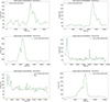 |
Fig. A.1. Background-subtracted 2−10 keV PN light curves (300 s bins) for the 2019 observations showing flares. Time zero corresponds to the observation start listed in Table A.1. |
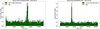 |
Fig. A.2. Background-subtracted 2−10 keV light curves of two bright flares detected in 2020−2022 (Obs.IDs 0862470501 and 0893811301). Time zero corresponds to the start of each observation. |
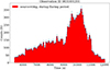 |
Fig. A.3. Combined source-plus-background light curve (MOS1+MOS2+PN) in the 2−10 keV band for 100 s bins during the August 31, 2019, flaring period (Obs.ID 0831801201). |
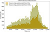 |
Fig. A.4. Combined background-subtracted light curves (MOS1+MOS2+PN) in the 2−10 keV band during the August 31, 2019, flaring period for 50 s and 100 s bins. |
List of all XMM-Newton observations from 2019
Best-fit Gaussian parameters for the August 31, 2019 flare.
All Tables
Characteristics of the five brightest Sgr A* flares detected by XMM-Newton (PN camera).
All Figures
|
Fig. 1. Sky image of Sgr A* from the XMM-Newton observation on August 31, 2019. The source extraction region is a circular aperture of radius 10″ centred on the very long-based interferometry radio position of Sgr A*. The background is extracted from an annulus with inner and outer radii of 175″ and 200″, respectively. |
| In the text | |
|
Fig. 2. Background-subtracted 2−10 keV PN light curves (300 s bins) of the five brightest X-ray flares detected from Sgr A*. The August 31, 2019 flare (Obs.ID 0831801201) is shown together with bright flares observed in 2002 (0111350301), 2007 (0402430401), 2014 (0743630201), and on March 16, 2019 (0831800601). Source counts are extracted from a circular region of radius 10″, and the background from an annulus with inner and outer radii of 175″ and 200″. Time zero corresponds to the start of each observation (see Table A.1). |
| In the text | |
|
Fig. 3. Summed background-subtracted 2−10 keV light curves detected by MOS1, MOS2, and PN for time bins of 300 s (left) and 100 s (right), within the common exposure time, for the August 31, 2019, observation (Obs.ID 0831801201). |
| In the text | |
|
Fig. 4. Combined background-subtracted 2−10 keV light curves detected by MOS1, MOS2, and PN during the flaring activity of the August 31, 2019, observation (5400−12 000 s). The soft (2−5 keV) and hard (5−10 keV) bands are shown, and the hardness ratio (hard/soft) is overplotted (see the right-hand axis). The temporal evolution of the hardness ratio indicates spectral variability during the flare. |
| In the text | |
|
Fig. 5. Background-subtracted light curves of Sgr A* for the August 31, 2019, observation (Obs.ID 0831801201), shown separately for MOS1, MOS2, and PN. Counts per bin are plotted for the soft (2−5 keV) and hard (5−10 keV) bands using 50 s and 100 s binning. Horizontal dashed lines indicate baseline levels, while dotted and dash-dotted lines show the 3σ and 5σ thresholds. Shaded regions highlight narrow substructures near 9600 s (hard band) and 10 900 s (soft band), with their central times marked by vertical lines. Bins with jump significances exceeding 3σ are indicated. |
| In the text | |
|
Fig. 6. Double-Gaussian (top) and three-Gaussian (bottom) fits to the summed light curve (counts vs time) of the August 31, 2019, Sgr A* flare. Time zero corresponds to the start of the observation (Table A.1). |
| In the text | |
|
Fig. A.1. Background-subtracted 2−10 keV PN light curves (300 s bins) for the 2019 observations showing flares. Time zero corresponds to the observation start listed in Table A.1. |
| In the text | |
|
Fig. A.2. Background-subtracted 2−10 keV light curves of two bright flares detected in 2020−2022 (Obs.IDs 0862470501 and 0893811301). Time zero corresponds to the start of each observation. |
| In the text | |
|
Fig. A.3. Combined source-plus-background light curve (MOS1+MOS2+PN) in the 2−10 keV band for 100 s bins during the August 31, 2019, flaring period (Obs.ID 0831801201). |
| In the text | |
|
Fig. A.4. Combined background-subtracted light curves (MOS1+MOS2+PN) in the 2−10 keV band during the August 31, 2019, flaring period for 50 s and 100 s bins. |
| In the text | |
Current usage metrics show cumulative count of Article Views (full-text article views including HTML views, PDF and ePub downloads, according to the available data) and Abstracts Views on Vision4Press platform.
Data correspond to usage on the plateform after 2015. The current usage metrics is available 48-96 hours after online publication and is updated daily on week days.
Initial download of the metrics may take a while.