| Issue |
A&A
Volume 709, May 2026
|
|
|---|---|---|
| Article Number | A50 | |
| Number of page(s) | 11 | |
| Section | Extragalactic astronomy | |
| DOI | https://doi.org/10.1051/0004-6361/202558005 | |
| Published online | 01 May 2026 | |
Multimessenger flare in the quasar PKS 0446+11
1
Max Planck Institute for Radio Astronomy, Auf dem Hügel 69, D–53121 Bonn, Germany
2
Department of Astronomy, University of Michigan, 323 West Hall, 1085 S. University Avenue, Ann Arbor, MI 48109, USA
3
Special Astrophysical Observatory of the Russian Academy of Sciences, Nizhny Arkhyz, 369167, Russia
4
Instituto de Astrofísica de Andalucía-CSIC, Glorieta de la Astronomía s/n, 18008 Granada, Spain
5
Department of Physics and Astronomy, Denison University, Granville, OH 43023, USA
6
Institute for Nuclear Research, 60th October Anniversary Prospect 7a, Moscow 117312, Russia
7
Lebedev Physical Institute, Leninskiy prospekt 53, Moscow 119991, Russia
8
Department of Physics and Astronomy, Purdue University, 525 Northwestern Avenue, West Lafayette, IN 47907, USA
9
CePIA, Astronomy Department, Universidad de Concepción, Casilla 160-C, Concepción, Chile
10
Black Hole Initiative, Harvard University, 20 Garden St, Cambridge, MA 02138, USA
11
Moscow Institute of Physics and Technology, Dolgoprudny, Institutsky per., 9 Moscow region, 141700, Russia
12
Crimean Astrophysical Observatory, 298409 Nauchny, Crimea
13
Owens Valley Radio Observatory, California Institute of Technology, Pasadena, CA 91125, USA
14
Physics Department, Lomonosov Moscow State University, 1-2 Leninskie Gory, Moscow 119991, Russia
★ Corresponding author: This email address is being protected from spambots. You need JavaScript enabled to view it.
Received:
6
November
2025
Accepted:
27
March
2026
Abstract
Context. The physical mechanisms driving neutrino and electromagnetic flares in blazars remain poorly understood.
Aims. We investigate a prominent multimessenger flare in the quasar PKS 0446+11 to identify the processes responsible for its high-energy emission.
Methods. We analyzed the IceCube-240105A high-energy neutrino event together with contemporaneous observations in the gamma-ray, X-ray, optical, and radio bands. We modeled the on- and off-flare spectral energy distributions (SEDs) within a single-zone leptohadronic framework. Multi-epoch VLBA observations from the MOJAVE program provide parsec-scale polarization data that complement the multiwavelength light curves.
Results. No significant time delay was detected between the neutrino arrival and the flares in different energy bands. This is consistent with an extremely small jet viewing angle below 1 deg, inferred from the parsec-scale polarization structure. The flare can be reproduced by the injection of a proton population and an increase in the Doppler factor from 18 to 24. We also detected an approximately 90 deg rotation of the EVPA in the parsec-scale core during the initial phase of the flare, indicating the emergence of a shock formed by the change in the bulk plasma speed.
Conclusions. Our comprehensive multimessenger analysis demonstrates that the extreme beaming and subdegree viewing angle of this distant blazar can account for the observed neutrino and electromagnetic activity. These findings strengthen the case for blazars as efficient accelerators of hadrons and significant contributors to the observed high-energy neutrino flux.
Key words: neutrinos / galaxies: active / galaxies: jets / radio continuum: galaxies / quasars: individual: PKS 0446+11
© The Authors 2026
 Open Access article, published by EDP Sciences, under the terms of the Creative Commons Attribution License (https://creativecommons.org/licenses/by/4.0), which permits unrestricted use, distribution, and reproduction in any medium, provided the original work is properly cited.
This article is published in open access under the Subscribe to Open model.
Open access funding provided by Max Planck Society.
1. Introduction
The growing dataset of high-energy astrophysical neutrinos, while still limited, provides unique opportunities to uncover connections with electromagnetic counterparts. Various electromagnetic observational indicators have been employed to identify population-level associations between blazars and neutrinos, with bright compact radio emission proving most effective as an indicator of neutrino emission. This effect stems from relativistic beaming, where both radio emission and neutrinos are observed predominantly along the jet axis (Plavin et al. 2025). Population studies have examined both the time-averaged properties of compact radio emission and radio flares coincident with neutrino detections (e.g., Plavin et al. 2020; Hovatta et al. 2021; Kouch et al. 2024).
Several individual blazars have exhibited clear electromagnetic flares coincident with high-energy neutrino events. TXS 0506+056 showed enhanced activity across the entire electromagnetic spectrum, from gamma rays (IceCube Collaboration 2018) to radio wavelengths (Kun et al. 2019). The quasar PKS 1502+106 displayed a pronounced radio flare (Kiehlmann et al. 2019), while remaining quiescent at other wavelengths. Its association with a high energy neutrio was revealed through population analysis by Plavin et al. (2020). The BL Lac object PKS 0735+178 produced several neutrino events detected simultaneously by four observatories, accompanied by multiwavelength flaring (Acharyya et al. 2023; Sahakyan et al. 2023; Prince et al. 2024; Bharathan et al. 2024; Paraschos et al. 2025; Kim & Kim 2025). An untriggered flare search by ANTARES identified a coincident neutrino-gamma-radio flare in the quasar PKS 0239+108 (Albert et al. 2024). A number of other blazars have also shown indications of enhanced electromagnetic emission temporally associated with neutrino detections (e.g., Kadler et al. 2016; Giommi et al. 2020; Liao et al. 2022; Eppel et al. 2023; Jiang et al. 2025; Perger et al. 2025). Nevertheless, clear and statistically significant coincidences between high-energy neutrinos and broadband electromagnetic flares remain rare. This motivates our investigation of the recent multimessenger event associated with the blazar PKS 0446+11.
The IceCube alert IceCube-240105A was announced in GCN Circulars 35485 and 35498 (IceCube Collaboration 2024a,b) as a track-like event of the BRONZE stream (see a description of the alert system and types of the alerts in Aartsen et al. 2017; Abbasi et al. 2023). This alert has an estimated false alarm rate of 2.64 events per year due to atmospheric backgrounds. The epoch of arrival is January 5, 2024, 12:27:42.57 UT. The J2000 positions have uncertainties on the 90% point spread function containment level, which include systematics: right ascension (RA)  deg, declination (Dec)
  deg.
deg.
These circulars have indicated two Fermi-detected blazars in the error region. One of them was the low-synchrotron-peaked quasar PKS 0446+11 with a redshift of 2.153 (Shaw et al. 2012) and a bright parsec-scale jet. Its J2000 VLBI sky coordinates are given by the Radio Fundamental Catalog (Petrov & Kovalev 2025) as RA 04:49:07.671103, Dec +11:21:28.59628, with an accuracy better than 0.2 mas (catalog version rfc_2025c). Its angular distance to the event position is 0.40°. The apparent VLBI speed of its relativistic jet was measured for two components in the units of the speed of light c by Lister et al. (2019) to be 6.72 ± 0.47 and 6.48 ± 0.76. Soon after the IceCube alert, many groups around the world announced the start of a major electromagnetic flare in PKS 0446+11 from gamma rays to radio, including the following references: Sinapius et al. (2024), Prince (2024), Woo et al. (2024), Sharpe et al. (2024), Garrappa et al. (2024), Eppel et al. (2024), Kovalev et al. (2024), Vlasyuk & Spiridonova (2025).
2. Observational data
2.1. The radio-to-gamma light curve and VLBA observations
To analyze the variable electromagnetic emission before and during the flare associated with the high-energy neutrino event, we used both our own observations and reduced public observations of PKS 0446+11 across the electromagnetic spectrum. The combined light curve around the neutrino event appears in Figure 1, while the full 20-year coverage is shown in Figure A.1. A set of 15 GHz polarization VLBA images of this blazar from the MOJAVE program is presented in Figure 2. We provide a detailed discussion of the observations, data processing, and calibration in Appendix A.
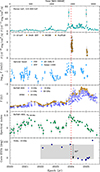 |
Fig. 1. Multiband light curve for PKS 0446+11, shown for the time range around the high energy neutrino arrival time. From top to bottom: Gamma ray, X-ray, optical, and radio light curves. They are supplemented by RATAN spectral index α, calculated for S ∝ ν+α between 5 and 22 GHz, and electric vector position angle (EVPA) of the parsec-scale core at 15 GHz, with a gray stripe of a 90° width. Uncertainties are shown as 1σ values. The IceCube-240105A neutrino event epoch is shown by the vertical dashed red line. See details in Section 2 and Appendix A. |
2.2. A collection of calibrated data for SED
For the purposes of the spectral energy distribution (SED) modeling (Section 3), we collected multiwavelength flux measurements, making use of the Markarian Multiwavelength Data Center (MMDC, Sahakyan et al. 2024) data collection tool. These include measurements from VLA (Lane et al. 2014; Gordon et al. 2021), GLEAM (Hurley-Walker et al. 2017), TGSS (Intema et al. 2017), Green Bank Observatory (White & Becker 1992; Gregory & Condon 1991; Gregory et al. 1996), RACS (Hale et al. 2021), NVSS (Condon et al. 1998), CRATES (Healey et al. 2007), Planck (Planck Collaboration Int. LIV 2018), ALMA (Bonato et al. 2019), WISE and NEOWISE (Wright et al. 2010; Mainzer et al. 2014; Schlafly et al. 2019), 2MASS (Skrutskie et al. 2006), PanSTARRS (Flewelling et al. 2020), SDSS (Abolfathi et al. 2018), Gaia (Gaia Collaboration 2016), ZTF (Bellm et al. 2019), UVOT (Yershov 2014), ASAS-SN (Hart et al. 2023), Swift (Giommi et al. 2019; Evans et al. 2020; Sahakyan et al. 2024), eROSITA (Merloni et al. 2024), and NuSTAR (Middei et al. 2022), along with data from Kuehr et al. (1981), Stein et al. (2021), Lasker et al. (2008), Yershov (2014). For explanations of the acronyms, we refer to the cited papers.
We supplement the data provided by MMDC with more data from ALMA (Bonato et al. 2019) and the data described in Appendix A. The data are split in two parts: “flare” (observation date 60 200 ≤ MJD ≤ 60 700) and “off-flare” (54 684 ≤ MJD ≤ 60 200 and historical catalog values). Individual observations at the same frequencies are averaged within these two time intervals, even if performed by different instruments. Fluxes are corrected for the Galactic extinction using the HI column density (HI4PI Collaboration 2016), its relation to the V-band extinction from Foight et al. (2016), and the color correction of Schlafly & Finkbeiner (2011).
2.3. Neutrino
The IceCube neutrino event associated with PKS 0446+11 was reported as an alert 240105A in the BRONZE stream (IceCube Collaboration 2024a,b) with the estimated best-fit energy1 of 109 TeV, while none were detected in the GOLD stream. The energy uncertainties may be estimated by scaling typical track alert energy errors (see, e.g., IceCube Collaboration 2018) to the best-fit energy of the present event; we obtain  TeV. We note that for muon tracks which cross the neutrino detector volume, strongly asymmetric errors in the energy estimate are typical. For the flux estimate, we use the effective area of ≈20 m2, as reported for the combined GOLD and BRONZE sample in the online tables2 accompanying the IceCat-1 catalog Abbasi et al. (2023) and interpolated to the best-fit neutrino energy of 109 TeV. Unfortunately the effective area is rather coarsely binned in declination (the bin we use is from 0° to +30°).
For the flare analysis, one event was used, and the Poisson confidence interval was adopted as  at 68% confidence level (CL). The neutrino flux is estimated as
  erg cm−2 s−1. This assumes the flare duration of 500 d, see the discussion in Section 3 and Fermi light curve analysis in Appendix B. For the off-flare period, no neutrino alerts associated with PKS 0446+11 were present and the Poisson upper limit of < 2.44 events at 90% CL was used. This resulted in a neutrino flux limit of 3.0 × 10⁻¹² erg cm−2 s−1.
3. A single-zone SED model
We used the data described above to obtain broadband SEDs of PKS 0446+11 for the off-flare and on-flare periods. These SEDs are presented in Figure 3 together with predictions of a single-zone leptohadronic model, obtained with the help of the publicly available simulation code AM3 (Klinger et al. 2024). The parameters of the model are listed in Table 1. In our simulation, we adopt a baseline scenario and assume the same ballistic escape time for all particles, tesc = R/c. Usually, SED modeling implies parameter degeneracy, so the solution presented here is a representative one, rather than unique. We note that Khatoon et al. (2026) have independently modeled the SED for PKS 0446+11, focusing on the period in early 2024.
Parameters of the SED model.
The AM3 code consistently takes into account standard electromagnetic processes: synchrotron emission, inverse Compton scattering and, where relevant, pair production, γγ → e+e−. Hadronic interactions with photons are modeled, including both those which lead to production of π mesons, whose subsequent decays generate high-energy neutrinos and photons, and Bethe-Heitler pair production, pγ → pe+e−. For the purpose of the present work we neglect pp interactions, whose probability is suppressed in blazar jets with respect to pγ interactions.
All secondary particles are tracked, so electromagnetic cascades initiated by the e+e− pair production and taking place in the source are followed down to photon escape energies. For the calculation of gamma-ray pair production on the extragalactic background light during their propagation from the source to the observer, we adopt the Gilmore et al. (2012) fiducial model of the extragalactic background light (EBL). For the redshift of PKS 0446+11, z = 2.153, the optical depth for gamma-ray energies > 100 GeV is τ ≳ 2.6 and rapidly grows with energy. This explains the sharp cutoff in the photon SED at these energies and makes it hardly possible to detect such energetic gamma rays from this source at the Earth, unless new physics affects the e+e− pair production.
All the processes relevant to both electromagnetic and neutrino emissions are assumed to take place in a spherical region (hereafter, a blob) through which the relativistic plasma flow is passing and where injected non-thermal electrons and protons interact. We might see from Table 1 that both the flare and off-flare SEDs are described by very similar parameters, with two key differences during the flare, in terms of both the proton luminosity and Doppler factor increase.
We verified that radiation fields external to the emission region have only a subdominant impact on the modeled SED. This includes the cosmic microwave background (CMB), accretion disk (AD), and broad-line region (BLR) emissions. The CMB contribution is negligible close to the jet base, where the photon field is dominated by the AGN emission. The influence of other external components depends on the location of the emitting blob. Assuming its preferred radius of 5 × 1016 cm (≈0.012 pc), the blob may still be located farther from the black hole. The key question is whether it resides within or beyond the BLR. Including a noticeable BLR contribution worsened the fit compared to the baseline model. We therefore conclude that the neutrino-emitting region lies beyond the BLR, at distances ≳0.1 pc from the black hole, where BLR photons are deboosted and contribute insignificantly. This is supported by an independent beaming analysis of Plavin et al. (2025), who deduced that neutrino production happens at sub-parsec distances, where the jet is already partly accelerated. The same reasoning applies to AD photons. This interpretation is supported by the absence of a strong X-ray cascade component, which would otherwise arise from interactions with BLR and AD photons. The inferred larger distance is also consistent with the relatively low magnetic field suggested by our model.
The small size of the region, however, suggests that it is located close to the jet base and not far from the central black hole, ≲0.5 pc, because it would expand adiabatically when moving to farther parts of the jet. This is supported by the fact that the SED does not describe radio measurements, for which the inner part of the jet is opaque. Data points in the radio band were used as the upper limit in our SED modeling and the corresponding emission is assumed to come from different parts of the jet.
The estimate of the neutrino flux, which determines the hadronic part of the SED model, depends crucially on the assumed duration of the flare. We note that the inspection of the gamma-ray light curve (cf. Figure 1) reveals two timescales of the flare: short peaks of a few-day duration and the main flare of 500 d. For a detailed analysis (see Appendix B). If the neutrino emission were associated with the short timescale, the flux estimate would increase by two orders of magnitude, making the observed SED impossible to explain because of the required unrealistic proton power. We consider this as an additional argument that the neutrino emission is associated with longer processes, namely, on the order of the duration of the main gamma-ray and radio flare.
The inferred parameters of the injected proton spectrum are quite unusual. The spectrum can be parametrized with a segment of a power law, with the minimal and maximal energies being free parameters, together with the spectral index. We find that a hard proton spectrum is needed to describe all the data and the difference between minimal and maximal energies is less than an order of magnitude. Attempts to describe the SED with a wider spectrum for protons fail because of an excessive contribution of secondary photons at the energies between the synchrotron and Compton bumps of the SED; this problem is also known for TXS 0506+056 (Gao et al. 2019). The most problematic contribution comes from electromagnetic cascades initiated by both Bethe-Heitler electrons and from energetic photons born in π0 decays. Variants of proton acceleration mechanisms, possibly operating in the jet and providing such hard and narrow spectra, include magnetic reconnection (e.g., Guo et al. 2014; Nalewajko 2016), the converter mechanism (Derishev et al. 2003), transrelativistic shocks (Bykov et al. 2022), etc. The observation of the high energy neutrino from PKS 0446+11 is a rare case where hints about the origin of accelerated protons may be obtained. This might be related to the extremely small viewing angle (Section 5), which opens access to a different combination of observables.
The on-flare value of the proton power injected in the neutrino emission zone, Lp, is an order of magnitude higher than the Eddington luminosity, LEdd, for a 109 M⊙ black hole. For a steady relativistic flow, the host-galaxy-frame jet power scales as Γ2 times the comoving energy density. Thus, compared to the comoving proton-injection power, the corresponding host-galaxy-frame power budget is ∼Γ2Lp, up to a factor of order unity. Importantly, LEdd is a limit on the radiative luminosity of quasi-spherical accretion, and not a strict upper bound on the jet power, which may be extracted from the black-hole rotation (Blandford & Znajek 1977). Simulations of jet launching in this regime confirm that the jet power can greatly exceed LEdd (e.g., Tchekhovskoy et al. 2011; Sądowski & Narayan 2015). Observationally, kinetic jet proton power exceeding the Eddington luminosity by a factor of ten may even be common (Ghisellini et al. 2014). Upper limits on the proton power instead come from the secondary radiation from the associated electromagnetic cascades (e.g., Murase et al. 2014; Reimer et al. 2019). This cascade emission is accounted for in our SED model and does not overshoot the data. Therefore, for PKS 0446+11, the required Lp > LEdd does not present a problem. The location of both the proton acceleration region and the neutrino production zone in the jet is consistent with observational results (e.g., Plavin et al. 2025; Kouch et al. 2026), which indicate that neutrino blazars are preferentially selected through Doppler boosting.
4. The 90 deg EVPA flip in the parsec-scale core
The epochs before and after the neutrino event demonstrate a clear 90° flip of the EVPA in the core region, as seen in the time series in Figure 1 and the polarization VLBI images in Figure 2. The polarization direction changes by about 90° within six months or less after the neutrino arrival and flips back approximately one year later. We note that the uncertainties in the measured core EVPA are about 5° or smaller.
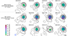 |
Fig. 2. Set of polarization MOJAVE images, observed by the VLBA at 15 GHz. The images are reconstructed using the CLEAN method and the same circular restoring beam, whose FWHM size of 0.7 mas is shown in the bottom-left corner. Stokes I is indicated by contours, with fractional polarization superimposed in false color. Stokes I contours start from a 4σ rms level. The EVPA is indicated by sticks. Drastic changes in the polarization direction around the neutrino arrival (January 5, 2024) are readily apparent (see also Figure 1). |
The 90° EVPA flip following the neutrino event may reflect (i) a substantial change in core opacity; (ii) the emergence of a shock; or (iii) an increase in its emission. Wardle (2018) noted that a very high synchrotron opacity of τ > 6 is required for the first scenario, which is observationally rare. Nevertheless, opacity-driven EVPA flips have been observed by Angelakis et al. (2017), Kosogorov et al. (2022, 2024).
In the case of PKS 0446+11, we concur with Wardle (2018) and do not associate the EVPA flip with opacity effects, for the following reason. As seen in Figure 1 and Figure 2, the core EVPA remained around +80° for at least two years prior to the neutrino’s arrival, despite significant variations in the spectral index, which became inverted at the end of 2023 during the start of the radio flare. After the neutrino arrival, the core EVPA shifted to about −10° and stayed there for nearly 1.5 years, while the radio flare exhibited two peaks and the spectral index varied between +0.5 and −0.3. Since the spectral index variations are the most direct indicator of changing opacity, we conclude that the flip is not related to opacity variations. Moreover, the core fractional linear polarization increased after the flip (Figure 2), whereas a strong increase in opacity is expected to reduce the fractional polarization (e.g., Angelakis et al. 2017).
We find that the emergence of a shock (or the enhancement of polarized emission associated with it) provides a more plausible explanation. Hughes et al. (1989) showed that a shock can produce both a 90° EVPA rotation and an increase in the fractional polarization, just as we observed (Figure 2). The polarized flux increases strongly after the neutrino arrival, likely dominating the original quiescent emission that might still persist in the unresolved core region.
Plavin et al. (2022) estimated the jet direction to be at the position angle of 121° ±4° at 15 GHz in the plane of the sky. We note that the core EVPA values before and after the flip do not agree with parallel and perpendicular jet directions, as could be expected for a shock enhancement. This might be explained by either the unknown Faraday rotation measure (RM being on an order of one and a half thousand rad m−2 is sufficient) or a change in the inner jet direction. The latter is realistic to expect in projection, due to the low assumed jet viewing angle (see the discussion in Section 5).
5. The jet viewing angle and Lorentz factor
For the off-flare and on-flare blob, with Doppler factors of δ = 18 & 24 (Table 1) and the apparent jet speed βapp = 6.7 c measured by MOJAVE (Lister et al. 2019), we obtain viewing angle estimates θ ≈ 2° & 1.2°, respectively. At the same time, βapp is measured at a projected distance on the order of 5 pc from the apparent jet base. The single-zone emitting blob is expected to be located significantly closer to the central engine (see discussion above), where the plasma may still undergo substantial acceleration (Homan et al. 2015; Kovalev et al. 2020) and the apparent speed is likely lower. Therefore, the values of βapp and θ quoted above should be regarded as upper limits.
We go on to consider the following. The very high energy photon and neutrino emitter PKS 1424+240 was found to have a strong toroidal component in a face-on jet with a viewing angle about or less than 0.6° (Kovalev et al. 2025). A radial EVPA pattern was also found by Homan et al. (2002) in a specific jet region of PKS 1510−089, observed face-on. The EVPA directions in the jet of PKS 0446+11 show a similar radial pattern at one epoch, where the core emission doesn’t dominate the jet, see Figure 4. Together with its wide apparent opening angle of 42° (Pushkarev et al. 2017), this strongly supports a very small jet viewing angle (i.e., smaller than its opening angle).
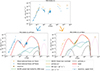 |
Fig. 3. Top: Combined Spectral Energy Distribution (SED) for the quasar PKS 0446+11. Bottom-left: the off flare period. Bottom-right: the on flare period. The total photon spectrum is shown as a thick red curve. The pink dashed line represents the neutrino spectrum (all flavors). The orange curve gives the sum of synchrotron and Compton emissions from injected electrons, while the black one is the synchrotron emission from injected protons. The green and blue curves present the secondary emission from e+e− pairs generated via the Bethe–Heitler process and γγ annihilation, respectively. See the text for discussion of the observational data points. |
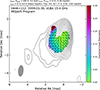 |
Fig. 4. MOJAVE 15 GHz VLBA epoch with the weakest core emission. Stokes I is shown by contours, while fractional linear polarization by false color and EVPA direction by sticks. Stokes I contours start from a 2.5σ level. The beam is presented at the FWHM level as an elliptical Gaussian in the bottom left corner. The radial pattern of the EVPA directions is readily apparent, indicating a close to face-on viewing angle, as described in Section 5. This effect clearly seen in epochs with low core dominance because of dynamic range limitations (cf. Figure 2). We note that the color bar in Figure 2 has a different scale, reflecting changes in the core polarization fraction over time. |
On this basis, we adopted θ = 0.6°, in line with Kovalev et al. (2025). The Lorentz factor depends only weakly on the viewing angle in this regime, becoming Γ ≈ 9 & 12 for the off-flare and on-flare periods, respectively. We note that an increase in the plasma Lorentz factor may lead to the formation of an associated shock (e.g., Spada et al. 2001), as discussed in Section 4.
6. Multimessenger flare coincidence and the gamma-ray-to-radio delay
A visual inspection of the light curve in Figure 1 reveals that the electromagnetic flare had its start a couple of months before the neutrino detection in all well-sampled bands (gamma ray, optical, and radio). The parsec-scale core brightness had also already increased significantly by the onset of the flare in late 2023. However, this does not necessarily imply that the neutrino flare was delayed relative to the electromagnetic one. Given the low statistics of neutrino detections, the observations are compatible with a range of scenarios, from simultaneous flares across all bands and messengers to constant neutrino emission over time. Nevertheless, we interpret this as a simultaneous multimessenger flare in PKS 0446+11.
Such a close temporal coincidence between the neutrino arrival and the broadband electromagnetic flare strongly suggests the neutrino emission is also flaring, making the situation qualitatively similar to that of TXS 0506+056. A simple a posteriori analysis yields a 2% chance coincidence probability based on temporal information alone. Among 314 VLBI-bright blazars (flux density ≥150 mJy in Petrov & Kovalev 2025) with radio and gamma-ray light curves available from OVRO and Fermi LAT monitoring, only six (including PKS 0446+11) exhibit gamma-ray and radio peaks within one year of the 5 January 2024 neutrino arrival. We also refer to Chen et al. (2025) for independent estimates.
The emission enhancement appears to begin simultaneously across all bands, from radio to gamma rays (Figure 1), with comparable timescales. Consequently (as noted in Section 3), we adopted the flaring scenario and assumed that the neutrino flare timescale is similar to that of gamma rays. This behavior is unusual compared with major flares in other neutrino-candidate blazars, including TXS 0506+056 (see references in Section 1). The gamma-ray-to-radio lag, Δt (e.g., Kramarenko et al. 2022), is typically related to the synchrotron opacity (e.g., Pushkarev et al. 2012): regions close to the jet origin are opaque to radio waves, but not to gamma rays. If the apparent base of a radio jet (radio “core”) is located at a de-projected distance, L, from the high-energy emitting blob (Section 3), the radio-to-gamma-ray delay is expected to be Δt = L sin θ/βapp from pure geometry. Pushkarev et al. (2012) estimated the typical de-projected distance between the true jet base and apparent 15 GHz parsec-scale core to be L ∼ 10 pc or ∼30 ly for the MOJAVE sample.
For the approximate calculations, we adopted the jet viewing angle of θ = 0.6° (Section 5). For the region of the high-energy blob close to the nucleus, we inferred an apparent speed of βapp = 3c, which corresponds to δ = 24 (Section 5). The apparent speed increases to 6.7c on parsec scales, as measured by MOJAVE (Lister et al. 2019). Under these conditions, the gamma-to-radio delay is expected to be Δt = 2–4 months in observer’s frame. This delay is consistent with the observed light curves for PKS 0446+11 and earlier studies by Pushkarev et al. (2017), Lister et al. (2019), Homan et al. (2021). Measuring this delay precisely is challenging due to the complex flaring behavior of the blazar.
7. Summary
This paper presents a detailed multiwavelength study of a prominent multimessenger flare from the quasar PKS 0446+11, which is temporally associated with the high-energy neutrino IceCube-240105A. Using contemporaneous gamma ray, X-ray, optical, and radio monitoring, complemented by parsec-scale radio imaging and archival spectral data, we characterized the flare’s timing, energetics, and SED.
We modeled the broadband SED and interpret the neutrino–electromagnetic flare by introducing a hadronic component and an increase in the Doppler factor within a single-zone framework. The parsec-scale polarization morphology indicates a very small viewing angle (i.e., about or below 0.6°) consistent with the observed apparent jet speed of about 6c and SED-fitted Doppler factors on the order of 20.
We discovered a 90° flip in the parsec-scale core linear polarization direction occurring after the neutrino detection. This suggests the emergence or strengthening of a shock emission region. Together with the nearly simultaneous flare starting time from gamma ray to radio, this supports a scenario where the high-energy emission originates near the jet base.
Our results indicate that proton-induced interactions within the jet are a plausible mechanism for producing the observed neutrino, while remaining consistent with electromagnetic constraints. Overall, we provide strong observational evidence linking the neutrino event to jet activity in PKS 0446+11 (i.e., with an a posteriori chance coincidence estimated at 2%). We highlight the importance of continued multimessenger observations to constrain the underlying emission physics.
Data availability
The polarization maps are available at the CDS via https://cdsarc.cds.unistra.fr/viz-bin/cat/J/A+A/709/A50
Acknowledgments
We are grateful to the anonymous referee, whose comments have significantly helped us to improve the manuscript. We thank Egor Podlesnyi for fruitful discussions of the SED modeling, Teresa Toscano and Aditya Tamar for useful comments on the manuscript. This research was funded by the European Union (ERC MuSES project No 101142396). A.V. Plavin is a postdoctoral fellow at the Black Hole Initiative, which is funded by grants from the John Templeton Foundation (grants 60477, 61479, 62286) and the Gordon and Betty Moore Foundation (grant GBMF-8273). The work by A.K.E, P.I.K., Y.A.K., A.V. Popkov, Y.V.S., and S.V.T. is supported in the framework of the State project “Science” by the Ministry of Science and Higher Education of the Russian Federation under the contract 075-15-2024-541. The views and opinions expressed in this work are those of the authors and do not necessarily reflect the views of these Foundations. This research made use of the data from the MOJAVE database maintained by the MOJAVE team (Lister et al. 2018), and from MMDC (Sahakyan et al. 2024). The CSS survey is funded by the National Aeronautics and Space Administration under Grant No. NNG05GF22G issued through the Science Mission Directorate Near-Earth Objects Observations Program. ZTF is supported by the National Science Foundation under Grants No. AST-1440341 and AST-2034437. This work is partly based on the data obtained with the RATAN-600 radio telescope and Zeiss-1000 and AS-500/2 optical reflectors at the Special Astrophysical Observatory of the Russian Academy of Sciences (SAO RAS). The National Radio Astronomy Observatory is a facility of the National Science Foundation operated under cooperative agreement by Associated Universities, Inc. This research has made use of the NASA/IPAC Extragalactic Database, which is funded by the National Aeronautics and Space Administration and operated by the California Institute of Technology.
References
- Aartsen, M. G., Ackermann, M., Adams, J., et al. 2017, Astropart. Phys., 92, 30 [Google Scholar]
- Abbasi, R., Ackermann, M., Adams, J., et al. 2023, ApJS, 269, 25 [CrossRef] [Google Scholar]
- Abolfathi, B., Aguado, D. S., Aguilar, G., et al. 2018, ApJS, 235, 42 [NASA ADS] [CrossRef] [Google Scholar]
- Acharyya, A., Adams, C. B., Archer, A., et al. 2023, ApJ, 954, 70 [NASA ADS] [CrossRef] [Google Scholar]
- Albert, A., Alves, S., André, M., et al. 2024, ApJ, 964, 3 [Google Scholar]
- Aliakberov, K. D., Mingaliev, M. G., Naugolnaya, M. N., et al. 1985, Astrofiz. Issled. Izv. Spets. Astrofiz. Obs., 19, 60 [Google Scholar]
- Angelakis, E., Myserlis, I., & Zensus, J. A. 2017, Galaxies, 5, 81 [Google Scholar]
- Arnaud, K. A. 1996, ASP Conf. Ser., 101, 17 [Google Scholar]
- Baars, J. W. M., Genzel, R., Pauliny-Toth, I. I. K., & Witzel, A. 1977, A&A, 61, 99 [NASA ADS] [Google Scholar]
- Bellm, E. C., Kulkarni, S. R., Graham, M. J., et al. 2019, PASP, 131, 018002 [Google Scholar]
- Bharathan, A. M., Stalin, C. S., Sahayanathan, S., Bhattacharyya, S., & Mathew, B. 2024, MNRAS, 529, 3503 [NASA ADS] [CrossRef] [Google Scholar]
- Blandford, R. D., & Znajek, R. L. 1977, MNRAS, 179, 433 [NASA ADS] [CrossRef] [Google Scholar]
- Bonato, M., Liuzzo, E., Herranz, D., et al. 2019, MNRAS, 485, 1188 [NASA ADS] [CrossRef] [Google Scholar]
- Bykov, A. M., Osipov, S. M., & Romanskii, V. I. 2022, J. Exp. Theor. Phys., 134, 487 [Google Scholar]
- Chen, R.-Q., Jiang, X., & Liao, N.-H. 2025, Res. Astron. Astrophys., 25, 115018 [Google Scholar]
- Condon, J. J., Cotton, W. D., Greisen, E. W., et al. 1998, AJ, 115, 1693 [Google Scholar]
- Derishev, E. V., Aharonian, F. A., Kocharovsky, V. V., & Kocharovsky, V. V. 2003, Phys. Rev. D, 68, 043003 [NASA ADS] [CrossRef] [Google Scholar]
- Drake, A. J., Djorgovski, S. G., Mahabal, A., et al. 2009, ApJ, 696, 870 [Google Scholar]
- Eppel, F., Kadler, M., Ros, E., et al. 2023, IAU Symp., 375, 91 [NASA ADS] [Google Scholar]
- Eppel, F., Kadler, M., Debbrecht, L., et al. 2024, ATel, 16399, 1 [Google Scholar]
- Evans, P. A., Page, K. L., Osborne, J. P., et al. 2020, ApJS, 247, 54 [Google Scholar]
- Flewelling, H. A., Magnier, E. A., Chambers, K. C., et al. 2020, ApJS, 251, 7 [NASA ADS] [CrossRef] [Google Scholar]
- Foight, D., Guver, T., Ozel, F., & Slane, P. 2016, ApJ, 826, 66 [NASA ADS] [CrossRef] [Google Scholar]
- Gaia Collaboration (Brown, A. G. A., et al.) 2016, A&A, 595, A2 [NASA ADS] [CrossRef] [EDP Sciences] [Google Scholar]
- Gao, S., Fedynitch, A., Winter, W., & Pohl, M. 2019, Nat. Astron., 3, 88 [NASA ADS] [CrossRef] [Google Scholar]
- Garrappa, S., Ofek, E. O., Ben-Ami, S., et al. 2024, ATel, 16407, 1 [Google Scholar]
- Gendreau, K. C., Arzoumanian, Z., Adkins, P. W., et al. 2016, SPIE Conf. Ser., 9905, 99051H [NASA ADS] [Google Scholar]
- Ghisellini, G., Tavecchio, F., Maraschi, L., Celotti, A., & Sbarrato, T. 2014, Nature, 515, 376 [NASA ADS] [CrossRef] [Google Scholar]
- Gilmore, R. C., Somerville, R. S., Primack, J. R., & Dominguez, A. 2012, MNRAS, 422, 3189 [NASA ADS] [CrossRef] [Google Scholar]
- Giommi, P., Brandt, C. H., Barres de Almeida, U., et al. 2019, A&A, 631, A116 [NASA ADS] [CrossRef] [EDP Sciences] [Google Scholar]
- Giommi, P., Padovani, P., Oikonomou, F., et al. 2020, A&A, 640, L4 [NASA ADS] [CrossRef] [EDP Sciences] [Google Scholar]
- Gordon, Y. A., Boyce, M. M., O’Dea, C. P., et al. 2021, ApJS, 255, 30 [NASA ADS] [CrossRef] [Google Scholar]
- Gregory, P. C., & Condon, J. J. 1991, ApJS, 75, 1011 [Google Scholar]
- Gregory, P. C., Scott, W. K., Douglas, K., & Condon, J. J. 1996, ApJS, 103, 427 [NASA ADS] [CrossRef] [Google Scholar]
- Guo, F., Li, H., Daughton, W., & Liu, Y.-H. 2014, Phys. Rev. Lett., 113, 155005 [Google Scholar]
- Hale, C. L., McConnell, D., Thomson, A. J. M., et al. 2021, PASA, 38, e058 [NASA ADS] [CrossRef] [Google Scholar]
- Hart, K., Shappee, B. J., Hey, D., et al. 2023, ArXiv e-prints [arXiv:2304.03791] [Google Scholar]
- Healey, S. E., Romani, R. W., Taylor, G. B., et al. 2007, ApJS, 171, 61 [Google Scholar]
- HI4PI Collaboration (Ben Bekhti, N., et al.) 2016, A&A, 594, A116 [NASA ADS] [CrossRef] [EDP Sciences] [Google Scholar]
- Homan, D. C., Wardle, J. F. C., Cheung, C. C., Roberts, D. H., & Attridge, J. M. 2002, ApJ, 580, 742 [Google Scholar]
- Homan, D. C., Lister, M. L., Kovalev, Y. Y., et al. 2015, ApJ, 798, 134 [Google Scholar]
- Homan, D. C., Cohen, M. H., Hovatta, T., et al. 2021, ApJ, 923, 67 [NASA ADS] [CrossRef] [Google Scholar]
- Hovatta, T., Lindfors, E., Kiehlmann, S., et al. 2021, A&A, 650, A83 [NASA ADS] [CrossRef] [EDP Sciences] [Google Scholar]
- Hughes, P. A., Aller, H. D., & Aller, M. F. 1989, ApJ, 341, 68 [NASA ADS] [CrossRef] [Google Scholar]
- Hurley-Walker, N., Callingham, J. R., Hancock, P. J., et al. 2017, MNRAS, 464, 1146 [Google Scholar]
- IceCube Collaboration (Aartsen, M. G., et al.) 2018, Science, 361, eaat1378 [NASA ADS] [Google Scholar]
- IceCube Collaboration. 2024a, GCN, 35485, 1 [Google Scholar]
- IceCube Collaboration. 2024b, GCN, 35498, 1 [Google Scholar]
- Intema, H. T., Jagannathan, P., Mooley, K. P., & Frail, D. A. 2017, A&A, 598, A78 [NASA ADS] [CrossRef] [EDP Sciences] [Google Scholar]
- Jester, S., Schneider, D. P., Richards, G. T., et al. 2005, AJ, 130, 873 [Google Scholar]
- Jiang, X., Liao, N.-H., Xue, R., Fan, Y.-Z., & Wei, D.-M. 2025, ApJ, 986, 110 [Google Scholar]
- Kadler, M., Krauß, F., Mannheim, K., et al. 2016, Nat. Phys., 12, 807 [Google Scholar]
- Khatoon, R., Böttcher, M., & Robinson, J. 2026, ApJ, 999, 245 [Google Scholar]
- Kiehlmann, S., Hovatta, T., Kadler, M., Max-Moerbeck, W., & Readhead, A. C. S. 2019, ATel, 12996, 1 [NASA ADS] [Google Scholar]
- Kim, Y.-S., & Kim, J.-Y. 2025, A&A, 699, A381 [NASA ADS] [CrossRef] [EDP Sciences] [Google Scholar]
- Klinger, M., Rudolph, A., Rodrigues, X., et al. 2024, ApJS, 275, 4 [NASA ADS] [CrossRef] [Google Scholar]
- Korolkov, D. V., & Pariiskii, I. N. 1979, S&T, 57, 324 [Google Scholar]
- Kosogorov, N. A., Kovalev, Y. Y., Perucho, M., & Kovalev, Y. A. 2022, MNRAS, 510, 1480 [Google Scholar]
- Kosogorov, N. A., Kovalev, Y. Y., Perucho, M., & Kovalev, Y. A. 2024, MNRAS, 528, 1697 [NASA ADS] [CrossRef] [Google Scholar]
- Kouch, P. M., Lindfors, E., Hovatta, T., et al. 2024, A&A, 690, A111 [NASA ADS] [CrossRef] [EDP Sciences] [Google Scholar]
- Kouch, P. M., Hovatta, T., Lindfors, E., et al. 2026, A&A, 708, A383 [Google Scholar]
- Kovalev, Y. Y., Nizhelsky, N. A., Kovalev, Y. A., et al. 1999, A&AS, 139, 545 [NASA ADS] [CrossRef] [EDP Sciences] [Google Scholar]
- Kovalev, Y. Y., Pushkarev, A. B., Nokhrina, E. E., et al. 2020, MNRAS, 495, 3576 [NASA ADS] [CrossRef] [Google Scholar]
- Kovalev, Y. Y., Plavin, A. V., Troitsky, S. V., et al. 2024, ATel, 16409, 1 [Google Scholar]
- Kovalev, Y. Y., Pushkarev, A. B., Gómez, J. L., et al. 2025, A&A, 700, L12 [NASA ADS] [CrossRef] [EDP Sciences] [Google Scholar]
- Kramarenko, I. G., Pushkarev, A. B., Kovalev, Y. Y., et al. 2022, MNRAS, 510, 469 [Google Scholar]
- Kuehr, H., Witzel, A., Pauliny-Toth, I. I. K., & Nauber, U. 1981, A&AS, 45, 367 [NASA ADS] [Google Scholar]
- Kun, E., Biermann, P. L., & Gergely, L. Á. 2019, MNRAS, 483, L42 [NASA ADS] [CrossRef] [Google Scholar]
- Lane, W. M., Cotton, W. D., van Velzen, S., et al. 2014, MNRAS, 440, 327 [Google Scholar]
- Lasker, B. M., Lattanzi, M. G., McLean, B. J., et al. 2008, AJ, 136, 735 [Google Scholar]
- Liao, N.-H., Sheng, Z.-F., Jiang, N., et al. 2022, ApJ, 932, L25 [NASA ADS] [CrossRef] [Google Scholar]
- Lien, A., Sakamoto, T., Barthelmy, S. D., et al. 2016, ApJ, 829, 7 [Google Scholar]
- Lister, M. L., Aller, M. F., Aller, H. D., et al. 2018, ApJS, 234, 12 [CrossRef] [Google Scholar]
- Lister, M. L., Homan, D. C., Hovatta, T., et al. 2019, ApJ, 874, 43 [NASA ADS] [CrossRef] [Google Scholar]
- Lott, B., Escande, L., Larsson, S., & Ballet, J. 2012, A&A, 544, A6 [NASA ADS] [CrossRef] [EDP Sciences] [Google Scholar]
- Mainzer, A., Bauer, J., Cutri, R. M., et al. 2014, ApJ, 792, 30 [Google Scholar]
- Masci, F. J., Laher, R. R., Rusholme, B., et al. 2019, PASP, 131, 018003 [Google Scholar]
- Merloni, A., Lamer, G., Liu, T., et al. 2024, A&A, 682, A34 [NASA ADS] [CrossRef] [EDP Sciences] [Google Scholar]
- Middei, R., Giommi, P., Perri, M., et al. 2022, MNRAS, 514, 3179 [NASA ADS] [CrossRef] [Google Scholar]
- Murase, K., Inoue, Y., & Dermer, C. D. 2014, Phys. Rev. D, 90, 023007 [Google Scholar]
- Nalewajko, K. 2016, Galaxies, 4, 28 [NASA ADS] [CrossRef] [Google Scholar]
- NASA& HEASARC. 2018, VizieR Online Data Catalog: B/swift [Google Scholar]
- Ott, M., Witzel, A., Quirrenbach, A., et al. 1994, A&A, 284, 331 [NASA ADS] [Google Scholar]
- Paraschos, G. F., Traianou, E., Debbrecht, L. C., Liodakis, I., & Ros, E. 2025, ApJ, 989, 208 [Google Scholar]
- Parijskij, Y. N. 1993, IEEE Antennas Propag. Mag., 35, 7 [CrossRef] [Google Scholar]
- Perger, K., Frey, S., Gabányi, K. É., & Kun, E. 2025, A&A, 698, L2 [NASA ADS] [CrossRef] [EDP Sciences] [Google Scholar]
- Perley, R. A., & Butler, B. J. 2013, ApJS, 204, 19 [Google Scholar]
- Perley, R. A., & Butler, B. J. 2017, ApJS, 230, 7 [NASA ADS] [CrossRef] [Google Scholar]
- Petrov, L. Y., & Kovalev, Y. Y. 2025, ApJS, 276, 38 [NASA ADS] [CrossRef] [Google Scholar]
- Planck Collaboration Int. LIV. 2018, A&A, 619, A94 [NASA ADS] [CrossRef] [EDP Sciences] [Google Scholar]
- Plavin, A., Kovalev, Y. Y., Kovalev, Y. A., & Troitsky, S. 2020, ApJ, 894, 101 [Google Scholar]
- Plavin, A. V., Kovalev, Y. Y., & Pushkarev, A. B. 2022, ApJS, 260, 4 [NASA ADS] [CrossRef] [Google Scholar]
- Plavin, A. V., Kovalev, Y. Y., & Troitsky, S. V. 2025, ApJ, 991, 33 [Google Scholar]
- Prince, R. 2024, ATel, 16397, 1 [Google Scholar]
- Prince, R., Das, S., Gupta, N., Majumdar, P., & Czerny, B. 2024, MNRAS, 527, 8746 [Google Scholar]
- Pushkarev, A. B., Hovatta, T., Kovalev, Y. Y., et al. 2012, A&A, 545, A113 [NASA ADS] [CrossRef] [EDP Sciences] [Google Scholar]
- Pushkarev, A. B., Kovalev, Y. Y., Lister, M. L., & Savolainen, T. 2017, MNRAS, 468, 4992 [Google Scholar]
- Reimer, A., Böttcher, M., & Buson, S. 2019, ApJ, 881, 46 [Google Scholar]
- Richards, J. L., Max-Moerbeck, W., Pavlidou, V., et al. 2011, ApJS, 194, 29 [Google Scholar]
- Sądowski, A., & Narayan, R. 2015, MNRAS, 453, 3213 [Google Scholar]
- Sahakyan, N., Giommi, P., Padovani, P., et al. 2023, MNRAS, 519, 1396 [Google Scholar]
- Sahakyan, N., Vardanyan, V., Giommi, P., et al. 2024, AJ, 168, 289 [NASA ADS] [CrossRef] [Google Scholar]
- Scargle, J. D., Norris, J. P., Jackson, B., & Chiang, J. 2013, ApJ, 764, 167 [Google Scholar]
- Schlafly, E. F., & Finkbeiner, D. P. 2011, ApJ, 737, 103 [Google Scholar]
- Schlafly, E. F., Meisner, A. M., & Green, G. M. 2019, ApJS, 240, 30 [Google Scholar]
- Sharpe, R., Santander, M., Acharyya, A., et al. 2024, ATel, 16453, 1 [Google Scholar]
- Shaw, M. S., Romani, R. W., Cotter, G., et al. 2012, ApJ, 748, 49 [CrossRef] [Google Scholar]
- Sinapius, J., Garrappa, S., Buson, S., Bartolini, C., & Pfeiff, L. 2024, ATel, 16398, 1 [Google Scholar]
- Skrutskie, M. F., Cutri, R. M., Stiening, R., et al. 2006, AJ, 131, 1163 [NASA ADS] [CrossRef] [Google Scholar]
- Spada, M., Ghisellini, G., Lazzati, D., & Celotti, A. 2001, MNRAS, 325, 1559 [NASA ADS] [CrossRef] [Google Scholar]
- Stein, Y., Vollmer, B., Boch, T., et al. 2021, A&A, 655, A17 [NASA ADS] [CrossRef] [EDP Sciences] [Google Scholar]
- Tchekhovskoy, A., Narayan, R., & McKinney, J. C. 2011, MNRAS, 418, L79 [NASA ADS] [CrossRef] [Google Scholar]
- Tsybulev, P. G. 2011, Astrophys. Bull., 66, 109 [Google Scholar]
- Tsybulev, P. G., Nizhelskii, N. A., Dugin, M. V., et al. 2018, Astrophys. Bull., 73, 494 [NASA ADS] [CrossRef] [Google Scholar]
- Udovitskiy, R. Y., Sotnikova, Y. V., Mingaliev, M. G., et al. 2016, Astrophys. Bull., 71, 496 [NASA ADS] [CrossRef] [Google Scholar]
- Valyavin, G., Beskin, G., Valeev, A., et al. 2022, Photonics, 9, 950 [Google Scholar]
- Vlasyuk, V. V., & Spiridonova, O. I. 2025, ATel, 17008, 1 [Google Scholar]
- Vlasyuk, V. V., Sotnikova, Y. V., Volvach, A. E., et al. 2023, Astrophys. Bull., 78, 464 [Google Scholar]
- Wardle, J. 2018, Galaxies, 6, 5 [Google Scholar]
- White, R. L., & Becker, R. H. 1992, ApJS, 79, 331 [NASA ADS] [CrossRef] [Google Scholar]
- Woo, J., Acharyya, A., Feng, Q., et al. 2024, ATel, 16417, 1 [Google Scholar]
- Wright, E. L., Eisenhardt, P. R. M., Mainzer, A. K., et al. 2010, AJ, 140, 1868 [Google Scholar]
- Yershov, V. N. 2014, Ap&SS, 354, 97 [NASA ADS] [CrossRef] [Google Scholar]
Appendix A: Electromagnetic observations of PKS 0446+11, data processing, and calibration
The partial (Figure 1) and full (Figure A.1) multimessenger light curves of the quasar PKS 0446+11 show the data used in this work. Their observations and calibration are discussed below.
A.1. Radio band
PKS 0446+11 has been regularly observed at the RATAN-600 radio telescope (Korolkov & Pariiskii 1979; Parijskij 1993) since 1997 as a part of a program monitoring VLBI-bright blazars. After the IceCube alert in the beginning of 2024, we initiated more frequent RATAN-600 observations of this source within the framework of our neutrino trigger program. RATAN-600 is a transit-mode telescope that allows to obtain quasi-simultaneous broad-band radio spectra. During the transit of a source across the meridian in about 5 minutes, flux densities at six frequency bands are measured: 0.96/1.2, 2.3, 4.7, 7.7/8.2, 11, and 22 GHz; central frequencies of two bands have changed during the monitoring due to receiver upgrades. The data reduction procedure is described in detail in Kovalev et al. (1999), Tsybulev (2011), Udovitskiy et al. (2016), Tsybulev et al. (2018). Flux density calibration was made using the calibration curve covering the declination range between −35° and +49°. It was constructed from observations of a set of calibrators: J0025−26, J0137+33, J0240−23, J0627−05, J1154−35, J1331+30 (3C 286), J1347+12, J2039+42 (DR 21), J2107+42 (NGC 7027), and J0542+49 (3C 147), see for details Baars et al. (1977), Ott et al. (1994), Aliakberov et al. (1985), Perley & Butler (2013, 2017). The characteristic cadence of the RATAN-600 observations of PKS 0446+11 ranged from one to several months before the IceCube alert and from one day to two weeks after it. In the paper, the RATAN-600 frequencies are denoted by their rounded values: 5, 8, 11, and 22 GHz. We do not use the data at 1 and 2 GHz in our analysis because they are affected by radio interference. The trigger program data from 2024-2025 were averaged in approximately two-weak bins for improving the signal-to-noise ratio.
The Owens Valley Radio Observatory (OVRO) 40-meter Telescope has been dedicated to monitoring a sample of ∼1830 blazars with a typical cadence of 3-4 days since January 2008. It uses dual-beam optics straddling the central focus point in double switching mode to minimize atmospheric effects. The cryogenic receiver is centered at 15 GHz with a 2 GHz equivalent noise bandwidth. A temperature stabilized noise diode is used to compensate for gain drifts. The quasar 3C 286 is used for absolute flux density calibration, with an assumed value of 3.44 Jy (Baars et al. 1977). Occasionally, the molecular cloud DR 21 is used, calibrated relative to 3C 286 using early OVRO 40 m data. The details of the observing method, observations and data reduction are presented by Richards et al. (2011).
The MOJAVE program (Monitoring Of Jets in Active galactic nuclei with VLBA Experiments) performs the longest monitoring of active galactic nuclei (AGN) by the VLBA at 15 GHz, producing the highest number of source epochs among all similar projects. This program started in 1994 with Stokes I observations, and since 2002 includes polarization measurements. See Lister et al. (2018) and references therein. Completely calibrated data in the form of visibility and image FITS files are made available in an online archive3. We note that typical MOJAVE EVPA (Electric Vector Position Angle) uncertainties are estimated as 2-3 deg. In this paper, we present and discuss EVPA values for the core region (Figure 1), deduced from MOJAVE-calibrated VLBA images (Figure 2). We adopt a more conservative error estimate of 5 deg for the core EVPA. The quasar PKS 0446+11 was originally observed for two epochs in 1998 as part of the project BG077, which targeted high redshift blazars. In 2002–2010 it was observed as a member of the complete MOJAVE sample with a main goal to determine jet kinematics (Lister et al. 2019). Its observations restarted in 2022, in support of MOJAVE-neutrino studies.
A.2. Optical band
Optical photometric data were obtained from two publicly available surveys. The Catalina Sky Survey (CSS; Drake et al. 2009)4 provides V-band light curves covering the period from 5 April 2005 to 9 February 2016. The original CSS magnitudes (Vcss) were transformed into the Johnson V system using the relation given by Drake et al. (2009)V = Vcss + 0.31 (B − V)2 + 0.04 , where the color index B − V was estimated from the median ZTF color ⟨g − r⟩ = 0.983 by applying the relation from Jester et al. (2005): g − r = 0.93 (B − V)−0.06 . The Zwicky Transient Facility (ZTF; Masci et al. 2019)5 contributes g- and r-band photometry between 20 March 2018 and 26 October 2024 (DR23). The optical study (mainly in the R-band) was carried out with the 0.5-metre AS-500/2 (January 2024 – September 2024) and 1-metre Zeiss-1000 (October 2024 – January 2025) optical reflectors of SAO RAS.
The observations with the optical telescope Zeiss-1000 were conducted with a CCD photometer in the Cassegrain focus, which is equipped with a 2048 × 2048 px back-illuminated E2V chip CCD 42-40. Details of the instrumental setup are described in Vlasyuk et al. (2023). The main characteristics of the instrumental complex of an AS-500/2 reflector are presented in Valyavin et al. (2022). To improve the system parameters, we have installed a smaller but more sensitive detector in July 2023: the back-illuminated electron-multiplying CCD camera Andor IXonEM+897 with 512×512 px chip. The typical integration time for observations of the blazar was 300 s for Zeiss-1000 and 90 s for AS-500/2. The optical data are collected from 14 observing nights between January 2024 and January 2025.
A.3. X-ray band
X-ray monitoring data were collected from multiple public archives. For the quiescent state, we used Swift-XRT and NuSTAR data retrieved from the public data collections (see Section 2.2). Within the flare period (MJD 60315–60351; 2024 January 6 to February 11), additional observations from Swift-XRT, NICER, and NuSTAR were included. The fluxes were homogenized to the 3–10 keV energy band and are shown in Figure 1.
NuSTAR data were taken from the Astronomer’s Telegram report of Woo et al. (2024) and converted to the 3–10 keV band. NICER data products were retrieved from the NICERMASTR database (Gendreau et al. 2016), and Swift-XRT products from the SWIFTMASTR database (NASA & HEASARC 2018). Swift-XRT and NICER spectra were fitted in XSPEC (Arnaud 1996) with an absorbed power-law model (tbabs*powerlaw), adopting a fixed Galactic hydrogen column density of NH = 2.48 × 1020 cm−2. No significant variability was detected across the flare epochs. The weighted mean flux in the 3–10 keV band is (3.11 ± 0.25)×10−12 erg cm−2 s−1 with a photon index Γ = 1.06 ± 0.05. These values are consistent with an independent analysis reported in Astronomer’s Telegrams: Sharpe et al. (2024) obtained from NICER an average photon index of Γ = 1.34 ± 0.25 and an average unabsorbed flux of (4.76 ± 1.32)×10−12 erg cm−2 s−1 in the 0.2–12 keV range, while Prince (2024) reported Swift-XRT fluxes of (4.0 ± 1.0)×10−12 and (4.4 ± 0.7)×10−12 erg cm−2 s−1 on January 6 and 8, respectively, with photon indices Γ = 1.4 ± 0.5 and Γ = 1.21 ± 0.22.
For SED modeling during the flare, we used one representative NICER epoch with the longest exposure (MJD 60327; 2024 January 18; ObsID 6736120108; exposure time 8996 s) rather than a combination of all epochs to avoid possible systematics due to imperfect background subtraction. We derived unabsorbed fluxes in four energy bins (0.3–1, 1–2, 2–5, and 5–10 keV; Figure 3, left). NICER results from Sharpe et al. (2024) are also included in the same plot and are in good agreement with our measurements.
A.4. Gamma-ray band
To construct the gamma-ray light curve, we applied the adaptive binning (Lott et al. 2012) to the data of the Fermi Large Area Telescope (LAT). This technique enables to reveal more details compared to fixed-binning, especially during bright flares, and allows to create a light curve with a constant relative flux uncertainty, which we set at the level of 20%. We used the current version of the Fermitools software package, v.2.2.0. A source model was produced by the script MAKE4FGLXML.PY setting the 4FGL-DR3 source catalog, GLL_IEM_V07.FITS as a Galactic interstellar emission model designed for point source analysis, Pass 8 Source front+back class events, and ISO_P8R3_SOURCE_V3_V1.TXT for the isotropic spectral template. The Region-of-Interest (RoI) around the target source was set to 20° and accumulated 123 point-like sources and no extended ones. The procedure GTSELECT produced data cuts within 0.1–300 GeV energy range and from 2008-08-04 to 2025-10-02 time range. Adaptive binning was performed using a normal-time arrow and assuming that the source spectrum is constant with time. To obtain more accurate fluxes of the target source, the fluxes of two bright sources in the RoI were taken into account. One of these sources is positionally associated with the quasar 0506+056 separated by  from 0446+112. The bin widths derived are distributed from about 1 day during the flares in 2024 and 2025 to 70 days for the low-state periods, with a median of 21 days.
Appendix B: A Bayesian block analysis of flares in the Fermi LAT light curve of PKS 0446+11
Following a non-parametric modeling technique developed by Scargle et al. (2013), we divided the Fermi LAT data into ten Bayesian blocks (Figure B.1) with a value of false positive probability p0 = 5.7 × 10⁻⁷, equivalent to about 5σ detection threshold in Gaussian statistics. This conservative value is typically adopted for structure analysis of light curves in high-energy astrophysics to robustly isolate flares or quiescence (e.g., Lien et al. 2016). We define the quiescent background level as a minimum flux among the derived Bayesian blocks, assuming that flare tails do not make a significant contribution to it. In this way, the low state (LS) is 0.85 × 10⁻¹¹ erg/cm2/s, reflecting the lowest source activity level. Using traditional determination of a flare as ten times the flux increase in the low state level, we selected two flares with all data points above the flare level: 2010.166–2010.440 (100 d duration, 20.5 × LS) and 2023.744–2025.113 (500 d duration, 24.5 × LS). There are two short spikes embracing the recent long flare. The durations of the left and right spikes are about 6 d and 11 d, respectively. We note that the neutrino event is not coincident with the left spike, as it is offset by 58 d.
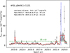 |
Fig. B.1. Fermi LAT light curve of PKS 0446+11 segmented by Bayesian blocks (red broken line). Two flares are identified, each exceeding ten times the level of the low state (green dashed line). The neutrino event epoch is marked by the blue dashed line. |
All Tables
All Figures
|
Fig. 1. Multiband light curve for PKS 0446+11, shown for the time range around the high energy neutrino arrival time. From top to bottom: Gamma ray, X-ray, optical, and radio light curves. They are supplemented by RATAN spectral index α, calculated for S ∝ ν+α between 5 and 22 GHz, and electric vector position angle (EVPA) of the parsec-scale core at 15 GHz, with a gray stripe of a 90° width. Uncertainties are shown as 1σ values. The IceCube-240105A neutrino event epoch is shown by the vertical dashed red line. See details in Section 2 and Appendix A. |
| In the text | |
|
Fig. 2. Set of polarization MOJAVE images, observed by the VLBA at 15 GHz. The images are reconstructed using the CLEAN method and the same circular restoring beam, whose FWHM size of 0.7 mas is shown in the bottom-left corner. Stokes I is indicated by contours, with fractional polarization superimposed in false color. Stokes I contours start from a 4σ rms level. The EVPA is indicated by sticks. Drastic changes in the polarization direction around the neutrino arrival (January 5, 2024) are readily apparent (see also Figure 1). |
| In the text | |
|
Fig. 3. Top: Combined Spectral Energy Distribution (SED) for the quasar PKS 0446+11. Bottom-left: the off flare period. Bottom-right: the on flare period. The total photon spectrum is shown as a thick red curve. The pink dashed line represents the neutrino spectrum (all flavors). The orange curve gives the sum of synchrotron and Compton emissions from injected electrons, while the black one is the synchrotron emission from injected protons. The green and blue curves present the secondary emission from e+e− pairs generated via the Bethe–Heitler process and γγ annihilation, respectively. See the text for discussion of the observational data points. |
| In the text | |
|
Fig. 4. MOJAVE 15 GHz VLBA epoch with the weakest core emission. Stokes I is shown by contours, while fractional linear polarization by false color and EVPA direction by sticks. Stokes I contours start from a 2.5σ level. The beam is presented at the FWHM level as an elliptical Gaussian in the bottom left corner. The radial pattern of the EVPA directions is readily apparent, indicating a close to face-on viewing angle, as described in Section 5. This effect clearly seen in epochs with low core dominance because of dynamic range limitations (cf. Figure 2). We note that the color bar in Figure 2 has a different scale, reflecting changes in the core polarization fraction over time. |
| In the text | |
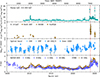 |
Fig. A.1. Full multiband light curve for PKS 0446+11. See detailed comments in Figure 1. |
| In the text | |
|
Fig. B.1. Fermi LAT light curve of PKS 0446+11 segmented by Bayesian blocks (red broken line). Two flares are identified, each exceeding ten times the level of the low state (green dashed line). The neutrino event epoch is marked by the blue dashed line. |
| In the text | |
Current usage metrics show cumulative count of Article Views (full-text article views including HTML views, PDF and ePub downloads, according to the available data) and Abstracts Views on Vision4Press platform.
Data correspond to usage on the plateform after 2015. The current usage metrics is available 48-96 hours after online publication and is updated daily on week days.
Initial download of the metrics may take a while.