| Issue |
A&A
Volume 709, May 2026
|
|
|---|---|---|
| Article Number | A1 | |
| Number of page(s) | 26 | |
| Section | Extragalactic astronomy | |
| DOI | https://doi.org/10.1051/0004-6361/202557583 | |
| Published online | 30 April 2026 | |
Spatially resolved interstellar dust properties in the face-on spiral galaxy M 99 as observed by NIKA2
1
Department of Physics and Astronomy, Universiteit Gent, Proeftuinstraat 86 N3, B-9000 Gent, Belgium
2
Université Paris-Saclay, Université Paris Cité, CEA, CNRS, AIM, 91191 Gif-sur-Yvette, France
3
Université Côte d’Azur, Observatoire de la Côte d’Azur, CNRS, Laboratoire Lagrange, France
4
School of Physics and Astronomy, Cardiff University, CF24 3AA, UK
5
Université Grenoble Alpes, CNRS, Grenoble INP, LPSC-IN2P3, 38000 Grenoble, France
6
Max Planck Institute for Extraterrestrial Physics, 85748 Garching, Germany
7
Aix Marseille Univ, CNRS, CNES, LAM, Marseille, France
8
Université Grenoble Alpes, CNRS, Institut Néel, Grenoble, France
9
Institut de RadioAstronomie Millimétrique (IRAM), Grenoble, France
10
Dipartimento di Fisica, Sapienza Università di Roma, I-00185 Roma, Italy
11
Univ. Grenoble Alpes, CNRS, IPAG, 38000 Grenoble, France
12
STAR Institute, Quartier Agora – Allée du six Août, 19c, B-4000 Liège, Belgium
13
INAF – Istituto di Radioastronomia, Via P. Gobetti 101, 40129 Bologna, Italy
14
Centro de Astrobiología (CSIC-INTA), Torrejón de Ardoz, 28850 Madrid, Spain
15
Institute for Research in Fundamental Sciences (IPM), School of Astronomy, Tehran, Iran
16
National Observatory of Athens, IAASARS, GR-15236 Athens, Greece
17
Faculty of Physics, University of Athens, GR-15784 Zografos, Athens, Greece
18
High Energy Physics Division, Argonne National Laboratory, Lemont, IL 60439, USA
19
Instituto de Radioastronomía Milimétrica (IRAM), Granada, Spain
20
LUX, Observatoire de Paris, PSL Research Univ., CNRS, Sorbonne Univ., UPMC, 75014 Paris, France
21
School of Earth & Space and Department of Physics, Arizona State University, Tempe, AZ 85287, USA
22
School of Physics and Astronomy, University of Leeds, Leeds LS2 9JT, UK
23
INAF-Osservatorio Astronomico di Cagliari, 09047 Selargius, Italy
24
LPENS, ENS, PSL Research Univ., CNRS, Sorbonne Univ., Université de Paris, 75005 Paris, France
25
Department of Physics and Astronomy, University of Pennsylvania, PA 19104, USA
26
Institut d’Astrophysique de Paris, CNRS (UMR7095), 75014 Paris, France
27
University of Lyon, UCB Lyon 1, CNRS/IN2P3, IP2I, 69622 Villeurbanne, France
28
Institut d’Astrophysique Spatiale (IAS), CNRS, Université Paris Sud, Orsay, France
29
IRAP, Université de Toulouse, CNRS, UPS, IRAP, Toulouse Cedex 4, France
30
Centre for Astrophysics – Harvard & Smithsonian, 60 Garden Street, 02138 Cambridge, MA, USA
31
National Radio Astronomy Observatory, 800 Bradbury SE, Suite 235 Albuquerque, NM 87106, USA
32
Institute of Astronomy and Astrophysics, Academia Sinica, No. 1, Sec. 4, Roosevelt Road, Taipei 106319, Taiwan
★ Corresponding author: This email address is being protected from spambots. You need JavaScript enabled to view it.
Received:
7
October
2025
Accepted:
15
February
2026
Abstract
Context. Large dust grains in thermal equilibrium dominate the far-infrared emission of star-forming galaxies and substantially contribute to their millimetre continuum. Constraining dust properties in this regime is challenging due to contamination from free-free and synchrotron emission.
Aims. We investigate the spatial variations in the dust spectral index, dust mass, and grain size and composition in the nearby face-on spiral galaxy M 99. To this end, we used new 1.15 and 2 mm continuum observations obtained with NIKA2 on the IRAM 30 m telescope as part of the IMEGIN Guaranteed Time Large Programme combined with ancillary data spanning ultraviolet to radio wavelengths.
Methods. We decomposed the infrared-to-radio spectral energy distribution of M 99 into dust, free-free, and synchrotron components using the hierarchical Bayesian spectral energy distribution fitting code HerBIE. We modelled the dust emission using both a modified blackbody (MBB) with a variable millimetre spectral index β and the THEMIS dust model with a fixed β. Our spatially resolved analysis was performed on ∼1.75 kpc (25″) scales, encompassing the galaxy centre, spiral arms, and inter-arm regions.
Results. From the MBB modelling, we found significant spatial variations in β, ranging from ∼1.6 − 1.7 in diffuse regions to ∼2.3 − 2.5 in denser star-forming environments. These variations likely reflect dust grain evolution driven by coagulation and changes in the silicate-to-carbonaceous grain abundance. Dust masses inferred with variable β are up to a factor of about four higher than those derived assuming a fixed β (1.6 on average). Variable-β models recover expected correlations with dust-to-stellar and dust-to-gas ratios, whereas fixed-β models systematically bias these quantities. The small grain fraction increases from ∼10% in the centre to ∼15% in the diffuse disc and is anti-correlated with the interstellar radiation field intensity, while gas-phase metallicity plays only a minor role within the central 8 kpc. The synchrotron spectral index varies from ∼0.6 − 0.7 in star-forming regions to ∼1.2 in the diffuse medium, consistent with cosmic ray electron ageing.
Key words: galaxies: ISM / galaxies: individual: M99 / galaxies: spiral
© The Authors 2026
 Open Access article, published by EDP Sciences, under the terms of the Creative Commons Attribution License (https://creativecommons.org/licenses/by/4.0), which permits unrestricted use, distribution, and reproduction in any medium, provided the original work is properly cited.
This article is published in open access under the Subscribe to Open model. This email address is being protected from spambots. You need JavaScript enabled to view it. to support open access publication.
1. Introduction
Interstellar dust grains are ubiquitous in galaxies and are generally well mixed with the gas in the interstellar medium (ISM; Galliano et al. 2018). Although they contribute only about 1% of the total ISM mass (Whittet 2022), dust grains play a significant role in shaping the spectral energy distribution (SED) of galaxies. They attenuate stellar light in the ultraviolet (UV) to optical range through absorption and scattering, and they re-emit the absorbed energy thermally in the infrared (IR; Whittet 2022).
Beyond studies of dust in the Milky Way (MW), observations of galaxies in the nearby Universe (within ∼100 Mpc) provide access to a wide diversity of environments, albeit at spatial resolutions typically limited to kiloparsec scales. Edge-on systems, for example, enable investigations of extraplanar dust at large vertical distances from the disc (e.g. Holwerda et al. 2012; Yoon et al. 2021; Chastenet et al. 2026), while face-on galaxies offer a favourable geometry for probing dust properties in the galaxy centre, spiral arms, and inter-arm regions as well as for characterising radial dust distributions (e.g. Casasola et al. 2017; Tailor et al. 2025). Spatially resolved studies of nearby galaxies hosting active galactic nuclei (AGNs; see Li 2007, for a review), dwarf galaxies (e.g. Rémy-Ruyer et al. 2013), and local starbursts (e.g. Contini & Contini 2003) have extended these investigations to extreme physical conditions. Collectively, observations of nearby galaxies constitute a crucial intermediate step towards understanding dust evolution across cosmic time and, in particular, in high-redshift systems (Galliano et al. 2018).
Several key open questions in dust studies concern the physical properties of dust grains at millimetre wavelengths. Robust constraints on the dust millimetre opacity (κ) and its slope (β; i.e. the dust spectral index) are essential for accurately deriving dust masses and for mapping dust-to-stellar, dust-to-gas, and dust-to-metal ratios (e.g. Lamperti et al. 2019). These quantities provide direct insight into the chemical evolution of galaxies and the reservoirs available for dust production (e.g. Casasola et al. 2022; Park et al. 2024).
Since 2017, the New IRAM KID Array 2 (NIKA2) camera installed on the IRAM 30 m telescope at Pico Veleta (Spain) has enabled continuum observations of galaxies at 1.15 and 2 mm, with angular resolutions of 12″ and 18″, respectively (Adam et al. 2018; Calvo et al. 2016; Perotto et al. 2020). Observations of nearby galaxies with NIKA2 provide a unique opportunity to spatially resolve dust emission in the millimetre regime and to directly probe variations in dust properties across different environments.
In this context, the IRAM 30 m Guaranteed Time Large Programme Interpreting the millimetre Emission of Galaxies with IRAM–NIKA2 (IMEGIN; PI: S. Madden) devoted approximately 200 hours to mapping the millimetre continuum of 22 nearby galaxies spanning a wide range of stellar masses, morphologies, and metallicities. The sample was selected to lie within 30 Mpc and to benefit from high-quality infrared-to-(sub)millimetre imaging for resolved SED modelling, complemented by matched-resolution UV, CO, and HI data. Notable results from the IMEGIN programme include the characterisation of extraplanar dust in the halo of NGC 891 (Katsioli et al. 2023), studies of dust emission in the starburst regions of NGC 2146 and in the peculiar dwarf galaxy NGC 2976 (Ejlali et al. 2025), and an analysis of dust properties in the barred spiral and AGN-host galaxy NGC 3627 (Katsioli et al. 2026).
As with other ground-based facilities, such as SCUBA-2 (e.g. Smith et al. 2021; Pattle et al. 2023), NIKA2 imaging of extended sources is subject to large-scale filtering. The severity of this filtering depends on a combination of atmospheric and instrumental noise, the observing strategy, and data reduction choices (e.g. source masking) and must be carefully quantified and accounted for in scientific analyses (see Appendix A.2 and Ejlali et al., in prep.).
This paper, part of the IMEGIN publication series, presents a spatially resolved analysis of the IR-to-radio emission of the nearby spiral galaxy M 99 (NGC 4254) based on SED fitting, with a particular emphasis on dust properties at millimetre wavelengths. M 99 is the first galaxy in the IMEGIN sample for which NIKA2 maps affected by large-scale filtering are analysed and published.
The M 99 spiral galaxy has a stellar mass of M★ ∼ 4.2 × 10¹⁰ M⊙ (Chemin et al. 2016), a star formation rate (SFR) ∼3.1 M⊙ yr−1 (Leroy et al. 2021), and an average gas-phase metallicity of 12 + log(O/H)∼8.6 (Kreckel et al. 2019), making it an excellent analogue to the MW. Its nearly face-on orientation, with an inclination of only 20 deg (Clark et al. 2018), offers a clear view of the galaxy centre, spiral arms, and disc. This favourable geometry is one of the primary motivations for selecting M 99 as a case study in the IMEGIN programme. Located at a distance of 14.40 Mpc (Poznanski et al. 2009), M 99 has an optical isophotal diameter of D25 ∼ 5′ (corresponding to ∼20 kpc; de Vaucouleurs et al. 1991; Clark et al. 2018). The galaxy exhibits a mild asymmetry in its morphology, characterised by a prominent spiral arm extending nearly 15 kpc perpendicular to the major axis in the optical band. This feature has been interpreted as a relic of a past tidal interaction with a massive companion, likely within the last gigayear (Soria & Wong 2006; Duc & Bournaud 2008; Chemin et al. 2016). The main geometric parameters of M 99 are summarised in Table 1.
List of the main geometric parameters for the face-on spiral galaxy M 99.
As part of the DustPedia (Davies et al. 2017; Clark et al. 2018) and KINGFISH (Kennicutt et al. 2011) samples, the integrated dust properties of M 99 have already been explored up to ∼500 μm (sampled by Herschel/SPIRE). Previous studies estimate a total dust mass of Mdust ∼ (2 − 5)×107 M⊙ (Nersesian et al. 2019; Aniano et al. 2020). In this work, we extend the analysis to the millimetre and radio regimes.
The structure of the paper is as follows. In Sect. 2, we present the NIKA2 observations of M 99, describe the ancillary datasets, and outline the procedures used to homogenise the multi-wavelength data. Sect. 3 details our SED fitting methodology. The results, both on integrated and spatially resolved scales, are presented and discussed in Sect. 4. Finally, we summarise our main conclusions in Sect. 5.
2. Data
2.1. NIKA2 observations at 1.15 mm and 2 mm
We observed M 99 with the IRAM 30 m/NIKA2 camera over multiple observing sessions conducted between February 2018 and January 2023. NIKA2 provides simultaneous continuum observations at 1.15 and 2 mm. The corresponding angular resolutions of 12″ and 18″ (FWHM) translate into linear scales of approximately 0.8 kpc and 1.25 kpc, respectively, at the distance of M 99. We acquired 159 scans, for a total of 24 hours of on-source integration time. Each sub-scan was conducted at speeds ranging from 40″ s−1 to 94″ s−1, with typical time separations of 10 s between sub-scans. Scanning directions alternated between position angles of 30 deg and 120 deg. For reference, each NIKA2 observing scan lasts approximately 420 s. Telescope pointing was updated hourly, and focus was adjusted every three hours. During observations, the elevation of the source ranged from 30 deg to 67 deg, while the atmospheric optical depth at 225 GHz (τ225 GHz) varied between 0.07 and 0.45, with a median value of 0.25.
The data were reduced using two independent pipelines: PIIC (Pointing and Imaging in Continuum; Zylka 2013; Berta & Zylka 2019) and Scanam_nika v14.0. The latter is adapted from the Scanamorphos algorithm originally developed for Herschel on-the-fly imaging (Roussel 2013) and subsequently optimised for NIKA2 observations (see Appendix A of Ejlali et al. 2025). Comparisons with space-based measurements (e.g. Planck) indicate that the PIIC maps suffer from substantial loss of extended emission, with up to ∼40% of the total flux filtered out at 1.15 mm (Ejlali et al., in prep.). In contrast, the Scanam_nika maps are consistent with Planck photometry once differences in filter transmission and central wavelength are taken into account. We further assess the reliability of the Scanam_nika products through dedicated simulations, in which the Herschel/SPIRE 250 μm map, convolved to the NIKA2 2 mm resolution, is processed identically to the NIKA2 data (see Appendix A.2 and Appendix A3 of Ejlali et al. 2025). These tests show that residual filtering of large-scale emission in the Scanam_nika maps varies on a pixel-by-pixel basis, reaching levels of up to ∼15%. We incorporate this effect into the flux density uncertainties, as described in Appendix A.2. Ejlali et al. (in prep.) will present a comprehensive overview of the data reduction methods (PIIC and Scanam_nika) applied to the IMEGIN sample and will describe the feathering of NIKA2 maps with data from cosmic microwave background (CMB) experiments (ACT or Planck). This technique generally enables the recovery of extended emission that is partially filtered out in some NIKA2 observations (see Smith et al. 2021). In this work, we adopted the Scanam_nika maps as our fiducial mm data products.
Figure 1 presents the final NIKA2 maps of M 99 in units of mJy px−1, with a pixel size of 3″. To convert the flux densities to mJy beam−1, beam areas of (188 ± 11) arcsec2 at 1.15 mm and (381 ± 11) arcsec2 at 2 mm should be used. The 1.15 mm map is constructed from 74 scans (out of 159), corresponding to ∼9.6 hours of usable on-source time; the remaining scans were excluded due to poor weather conditions or data corruption. The 2 mm map includes 151 scans (∼16.3 hours), with only 8 scans discarded. The selected scans span atmospheric opacities of 0.22 − 0.54 at 1.15 mm and 0.14 − 0.69 at 2 mm. The peak flux density in the 1.15 mm map is ∼0.6 mJy px−1 and ∼0.08 mJy px−1 at 2 mm. We measure the median sky brightness and root mean square (RMS) noise outside the source mask, ensuring inclusion of residual correlated noise. The sky level is then subtracted from the map as the final step of the Scanam_nika processing pipeline. The RMS is ∼0.034 mJy px−1 at 1.15 mm ∼0.006 mJy px−1 at 2 mm.
 |
Fig. 1. NIKA2 maps of M 99 at 1.15 mm (left) and 2 mm (right) obtained through the Scanam_nika data reduction pipeline in mJy px−1 (cutouts of 8′×6′; pixel size of 3″). The mean RMS is 0.034 mJy px−1 at 1.15 mm and 0.0055 mJy px−1 at 2 mm. White solid lines show the [2.5, 5, 7.5]×σ contours. The FWHM is ∼12″ at 1.15 mm and ∼18″ at 2 mm, corresponding to ∼0.8 and ∼1.25 kpc (see the white circles, bottom-left). |
2.2. Ancillary data
The M 99 galaxy is part of the DustPedia sample (Davies et al. 2017; Clark et al. 2018), which comprises 875 nearby galaxies with homogeneous multi-wavelength continuum coverage from the far-ultraviolet (FUV) to the mm regime. From DustPedia1 we used (i) the UV maps from GALEX (Martin et al. 2005) to calibrate the spatially resolved SFR surface density (not used in the SED modelling); (ii) the IR maps from Spitzer (Werner et al. 2004) and Herschel (Pilbratt et al. 2010) for SED modelling and Spitzer/MIPS maps to calibrate the stellar mass and SFR, as detailed in Appendix B; (iii) the Planck 1.38 mm map to model the integrated millimetre emission of M 99 (Sect. 4.1) and validate the total flux recovered by NIKA2 (Appendix A.3).
Spitzer/IRAC images are calibrated for point sources and require surface brightness corrections when applied to extended objects, such as nearby galaxies. Following Sect. 8.2 of the IRAC Instrument Handbook (v4.0; IRAC Instrument & Instrument Support Teams 2021), we apply correction factors of 0.91, 0.94, 0.66, and 0.74 to the 3.6, 4.5, 5.8, and 8.0 μm maps, respectively. The accuracy of these corrections (i.e., about 10%) is included in the systematic uncertainty reported in Table 2.
Multi-wavelength continuum maps used in this work.
We supplemented the DustPedia dataset with new and archival radio continuum maps from the Karl G. Jansky Very Large Array (VLA; Perley et al. 2011) and the Effelsberg 100 m Radio Telescope (Wielebinski et al. 2011). In Table 2 we provide a complete list of the continuum maps used in this work. We also incorporate full HI and CO maps (Table 3), along with ∼1900 gas-phase metallicity measurements from the literature (De Vis et al. 2019; Kreckel et al. 2019).
Spectral line intensity maps used in this work.
This comprehensive multi-wavelength data set enables the construction of spatially resolved maps of stellar mass, SFR, and atomic and molecular gas surface densities using widely adopted empirical calibrations. The maps identified as ‘calibrators’ in Table 2 are used as inputs for these derivations. In addition, we construct a map of the gas-phase metallicity of M 99, extending out to 2′ (∼8.4 kpc) from the galactic centre. Further details on the construction of these ancillary products are provided in Appendix B.
2.3. Data processing and homogenisation
Spatially resolved SED modelling requires all input maps to be homogenised in angular resolution, pixel scale, orientation, and units. In addition, the images must be corrected for potential contamination from astrophysical sources (e.g. bright foreground stars), large-scale foreground or background emission, instrumental artefacts or residual gradients.
To meet these requirements, we developed and applied the Homogenisation for IMEGIN Photometry post-processing pipeline (HIP)2. HIP performs several key steps: (i) identification and masking of bright foreground stars in the NIR images; (ii) modelling and subtraction of sky emission and instrumental gradients, particularly relevant for the GALEX, Spitzer, and Herschel datasets; (iii) estimation and removal of CO(2–1) line contribution from the NIKA2 1.15 mm and Planck/HFI4 continuum bands; (iv) measurement of integrated photometry; (v) convolution to a common angular resolution followed by reprojection to a uniform pixel scale and orientation. Uncertainties are propagated through these steps using either a bootstrap Monte Carlo (MC) approach or a faster gradient-based propagation method, validated against MC runs with NMC ∼ 103 − 104 iterations. In this work, we use NMC = 103 to generate uncertainty maps and NMC = 100 to estimate uncertainties on integrated fluxes.
Using HIP, we convolved the multi-wavelength maps of M 99 to the poorest angular resolution among the images included in each analysis, balancing adequate far-infrared (FIR) sampling with the high resolution of NIKA2. For the global analysis (Sect. 4.1), we used all maps listed in Table 2. For the analysis of the three morphological components of M 99 (disc, spiral arms, and galaxy centre; Sect. 4.2), we convolved the maps to 18″ (∼1.25 kpc), excluding the SPIRE 350 μm, SPIRE 500 μm, and Planck/HFI4 bands. For the pixel-by-pixel analysis (Sect. 4.3), we convolved the maps to 25″ (∼1.75 kpc), corresponding to the SPIRE 350 μm resolution, and resampled them onto an 8″ (∼0.56 kpc) pixel grid, excluding the SPIRE 500 μm and Planck/HFI4 data.
A detailed description of HIP is provided in Appendix C. There, we also describe the specific prescriptions adopted in this work.
3. SED fitting
We derived the dust properties of M 99 through SED fitting. Specifically, we employed the hierarchical Bayesian dust SED fitting code HerBIE (Galliano 2018; Galliano et al. 2021).
3.1. HerBIE: Hierarchical Bayesian SED fitting
HerBIE uses a hierarchical Bayesian framework to fit physical dust models, including realistic optical properties, stochastic heating, and a mixture of radiation environments. Unlike least-squares or non-hierarchical Bayesian methods, the hierarchical approach suppresses noise-driven correlations and scatter, yielding more accurate parameter estimates and uncertainties (Shetty et al. 2009; Kelly et al. 2012; Lamperti et al. 2019).
As for any Bayesian approach, HerBIE computes posterior probability density functions (PDFs) as the product of the likelihood and a prior. When the data poorly constrain a parameter, the prior dominates. In the hierarchical Bayesian application to our spatially resolved M 99 data, the priors are estimated from the ensemble of all pixels via a set of shared hyperparameters. These hyperparameters describe the distribution of physical parameters (e.g. dust mass, temperature) across all pixels in the maps and influence the posteriors of each individual pixel (Galliano 2018, Eq. (19)). Posterior distributions are sampled using a Gibbs-within-Metropolis-Hastings Markov chain Monte Carlo (MCMC) algorithm (Geman & Geman 1984). Finally, HerBIE explicitly accounts for both statistical and systematic uncertainties in the input maps (see Sect. 3 of Galliano 2018).
3.2. Physical components of the HerBIE SED model
We modelled the NIR-to-radio SED of M 99 using three distinct emission components. These comprise (i) dust emission in the MIR-to-millimetre range; (ii) the stellar continuum in the NIR; and (iii) the radio continuum, including both free–free and synchrotron emission.
The dust emission is described by the non-uniformly illuminated dust mixture model (powerU; Galliano 2018, Eq. (11)). It assumes the dust mass is illuminated with a range of radiation field intensities, U, following a power-law distribution (e.g. Dale et al. 2001). The dust emission was thus modelled with six free parameters: Umin, the minimum radiation field intensity; ΔU, the range of radiation field intensities; αdust, the spectral index describing the power-law distribution of radiation field intensities; Mdust, the total dust mass; q, the small-grain mass fraction; and q+, the fraction of charged small grains.
The NIR stellar continuum was modelled (using the starBB module) as a blackbody with T★ = 5 × 10⁴ K, ensuring the spectrum lies in the Rayleigh–Jeans regime. In HerBIE this component is described by a single free parameter, the bolometric luminosity, L★.
The radio continuum, comprising both free–free and synchrotron emission, is modelled (using the radio module) as two power laws (Galliano 2018, Eq. (13)) with three free parameters: Lradio, the luminosity at λ = 1 cm; fFF, the fraction of free-free emission at λ = 1 cm; and αsync, the synchrotron spectral index, assumed to be constant across the modelled range of frequencies.
In total, our SED fits involve ten free parameters. In the following, we refer to the mass-weighted starlight intensity heating the dust grains ⟨U⟩, as the average interstellar radiation field (ISRF). This quantity is a function of three underlying parameters: Umin, ΔU and αdust, for which the adopted priors are 0.01 < Umin < 1000; 0 < ΔU < 106; 1 < αdust < 2.5. Other prior ranges are summarised in Table 6.
An equivalent equilibrium temperature for large grains, Teq, can be estimated from:
 (1)
(1)
where ⟨U⟩ is normalised to the average ISRF in the solar neighbourhood, i.e. ⟨U⟩⊙ = 2.2 × 10⁻⁵ W m−2 (Mathis et al. 1983), and β is the dust spectral (e.g., Aniano et al. 2012; Nersesian et al. 2019).
3.3. THEMIS: A laboratory-based dust model
We adopted the physically motivated THEMIS dust model (Jones et al. 2013, 2017; Köhler et al. 2014) as the basis for the powerU component in HerBIE. THEMIS dust properties are anchored in laboratory measurements of the optical properties of interstellar dust analogues. THEMIS dust mixture is comprised of: (i) small (radius a < 150 nm), partially hydrogenated amorphous carbon grains, the smallest of which (a ≲ 10 nm) exhibit spectroscopic properties similar to polycyclic aromatic hydrocarbons (PAHs) and are responsible for the aromatic and aliphatic features observed in the MIR; (ii) large dehydrogenated amorphous carbon and silicate grains dominating the FIR continuum. Carbonaceous grains with a > 20 nm are coated with an amorphous carbon mantle, while silicate grains have both a carbon mantle and iron inclusions.
In HerBIE, the small, partially hydrogenated, amorphous carbon grains (AC) are modelled using three size-based populations: (i) very small (VSAC, a < 0.7 nm) grains are responsible for the shortest-wavelength MIR aromatic features; (ii) small (SAC, 0.7 < a < 1.5 nm) grains dominate the longer-wavelength MIR features; and (iii) medium/large (MLAC, a > 1.5 nm) grains produce the featureless MIR continuum and contribute to the FIR peak and long-wavelength continuum.
We defined the mass fraction of aromatic feature carriers qAF as qAF = qVSAC + qSAC where q denotes the mass fraction. This definition is analogous to the PAH mass fraction (qPAH) introduced by Draine & Li (2007)3.
The default THEMIS composition has 69% silicates, 14% MLAC, and 17% VSAC+SAC by mass. In our HerBIE fits, we adopted the default THEMIS grain properties but allow qAF to vary. The intrinsic dust millimetre spectral index (i.e. determined by the chemical composition of large grains) is thus constant, with β = 1.79 (Bianchi et al. 2019) for a given interstellar field intensity U, but mixing multiple U components can flatten the effective (i.e. observed) slope. This effect is illustrated, for example, in Fig. III.13 of Galliano (2022) and in Galliano (2018).
3.4. Single-temperature modified blackbody
In addition to the THEMIS dust model, we employ a single-T modified blackbody (MBB) model to describe the FIR SED of M 99, which is referred to as MBB1 in the HerBIE framework (Galliano 2018, Eq. (2)). The MBB model describes the thermal emission from dust grains heated by the ISRF. The free parameters are three: the dust mass, Mdust; the dust temperature, Tdust; and the dust spectral index, β.
This simplified model assumes that the FIR dust emission is dominated by a single temperature component, which is a reasonable approximation for wavelengths longer than 100 μm. A key advantage of using the MBB approach is that it allows us to explore spatial or environmental variations in β, which is otherwise fixed in the THEMIS model.
4. Results and discussion
In this Sect., we present our results and discuss their implications. As the hierarchical Bayesian framework is primarily designed for spatially resolved analyses, we performed the integrated SED fitting using HerBIE in its non-hierarchical mode.
4.1. A global view of the dust in M 99
We measured the integrated multi-wavelength photometry of M 99 (Table 4) using HIP (Appendix C.5), within the elliptical aperture shown in Fig. C.4, based on the geometry from Clark et al. (2018). Prior to extraction, we subtracted the sky emission (Appendix C.2) and corrected the NIKA2 1.15 mm and Planck/HFI4 maps for CO(2–1) contamination (Appendix C.6). Additional integrated properties of M 99 are summarised in Table 5. Our photometric measurements agree within uncertainties with DustPedia (Clark et al. 2018), KINGFISH (Aniano et al. 2020; Chang et al. 2020; Chastenet et al. 2025), and the 3 and 6 cm measurements of Tabatabaei et al. (2017). Fig. 2 shows the integrated SED of M 99 fitted with the THEMIS and MBB models. THEMIS reproduces the data well (χred2 = 1.35), though it slightly underestimates the steepness of the FIR slope. The MBB fit (λ ≳ 100 μm), instead, gives a better match in the FIR-mm (χred2 = 0.43). The MBB fit yields Mdust = (3.8 ± 0.7)×107 M⊙, dust temperature Tdust = 23.7 ± 0.9 K, and spectral index β = 1.85 ± 0.09 (Table 6). The MBB β is marginally steeper than the default THEMIS value (β = 1.79), although the two are consistent within the uncertainties. From the THEMIS fit, we derive Mdust = (3.2 ± 0.2)×107 M⊙ and, using Eq. (1), an equivalent temperature Teq ∼ 24.2 K, which is consistent with the MBB outcome. The dust-to-stellar and dust-to-gas ratios inferred from our dust mass estimates (Table 6) are typical of local star-forming spirals (e.g. Boselli et al. 2010; De Vis et al. 2017a; Aniano et al. 2020; Casasola et al. 2020, 2022).
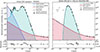 |
Fig. 2. Integrated NIR-to-radio SED modelling of M 99 with HerBIE. Filled black circles show observed photometry used in the fit; grey diamonds indicate corresponding synthetic photometry. Left panel: Full SED fit (black line), including stellar emission (starBB, blue), dust emission using powerU with THEMIS (green), and radio continuum (radio, red). Right panel: Fit limited to λ ≥ 100 μm using a single-T MBB (MBB1, green), excluding stellar emission. Empty circles denote data not included in the fit. Residuals are shown below each panel. |
Multi-band integrated photometry of M 99 computed with HIP.
Integrated properties of M 99 used in this work.
Best-fit parameter values obtained with HerBIE (non-hierarchical Bayesian framework) and derived quantities.
About 15% of the THEMIS dust mass is in small, partially hydrogenated carbonaceous grains (VSAC + SAC). THEMIS typically yields higher mass fractions of these grains than other models such as Draine & Li (2007) or Compiègne et al. (2011) because the carriers are less emissive (Galliano et al. 2021; Galliano 2022). For comparison, using the Draine & Li (2007) model, Aniano et al. (2020) derived, for M 99, qPAH = (4.1 ± 0.8)% and Mdust = (5.2 ± 0.4)×107 M⊙, while Chastenet et al. (2025) found qPAH = (4.4 ± 0.2)% and Mdust = (7.5 ± 0.6)×107 M⊙. The latter estimate is consistent with our dust masses after applying the recommended 1/3 scaling (e.g. Chastenet et al. 2021). We note that Draine & Li (2007) model has previously been shown to produce a higher dust mass than other physical ISM dust models by a factor of ∼2 (e.g. Galliano et al. 2011; Dalcanton et al. 2015; Galliano 2018).
Earlier studies of the integrated SED of M 99 by the DustPedia collaboration adopted THEMIS-like grains: Nersesian et al. (2019) obtained Mdust = (2.2 ± 0.1)×107 M⊙ with CIGALE, and (2.6 ± 0.2)×107 M⊙ from an MBB fit; Galliano et al. (2021) found (2.1 ± 0.2)×107 M⊙ using HerBIE. These dust masses are slightly lower than ours, likely due to methodological differences, although the dust temperatures (24 − 25 K) agree well with our estimates.
The new NIKA2 and radio observations enable a clear separation of the dust, free-free, and synchrotron components in the integrated SED of M 99. Dust emission dominates at 1.15 mm (∼99%), but its contribution decreases to 91% at 2 mm, 21% at 5 mm, and less than 2% at 1 cm. Adopting the THEMIS best-fit free-free fraction at 1 cm (fff = 0.15; Table 6), free-free emission contributes 52% of the radio continuum at 1.15 mm, declining to 40% at 2 mm and 23% at 5 mm, while synchrotron emission dominates at λ > 1 cm. The radio parameters derived from the MBB fit ( and
and  %) are consistent within uncertainties with those obtained using the THEMIS model. However, the MBB fit allows for higher free-free fractions (up to ∼50–60%), in line with typical values reported for normal star-forming galaxies (fff ∼ 50%; Condon 1992).
4.2. Dust properties in the centre, spiral arms, and disc of M 99
The nearly face-on orientation of M 99 allowed us to examine dust properties in the galaxy centre, spiral arms, and disc. To isolate these components, we adopted the morphological masks from Querejeta et al. (2021, PHANGS), which are based on the Spitzer/IRAC 3.6 μm map (see Fig. 3).
 |
Fig. 3. PHANGS environmental masks by Querejeta et al. (2021) degraded to match SPIRE 250 μm angular resolution (i.e. 18″ ∼ 1.25 kpc) and pixel size (i.e. 6″ ∼ 0.4 kpc). We show the disc in cyan, the spiral arms in blue, and the centre in magenta. For reference, we overlay the IRAC 3.6 μm contours (black solid lines). |
We integrated the flux densities of each component using HIP (Appendix C) and fit the resulting integrated SEDs with HerBIE (Galliano 2018), as detailed in Sect. 3. The multi-wavelength fluxes for the centre, spiral arms, and disc of M 99 are reported in Table 7. Their sum is consistent with the integrated photometry in Table 4.
Multi-band photometry of the spiral arms, disc, and centre of M 99 computed with HIP.
Figure 4 shows the integrated SEDs and their decomposition into stellar (THEMIS only), dust, and radio components. Table 8 lists the best-fit parameters, and Table 9 summarises the derived ISM properties. We note that these values average over large ISM volumes (a few kiloparsecs to ∼10 kpc) and encompass a mix of ISM environments, from molecular clouds and HII regions to diffuse media.
 |
Fig. 4. Near-IR-to-radio SED modelling of the spiral arms (blue), disc (cyan), and centre (magenta) of M 99 with HerBIE. Filled circles show observed photometry; grey diamonds indicate synthetic photometry. Left panel: Full SED fits (solid lines) including stellar emission (starBB, yellow areas); dust emission, using powerU with THEMIS (blue, cyan, magenta areas); and the radio continuum (radio, red areas). Right panel: Fits restricted to λ ≥ 100 μm, modelling dust with single-T MBB (MBB1, coloured areas), and excluding stellar emission. Empty circles were not included in the fit. Monochromatic luminosities (ν Lν) assume a distance of 14.4 Mpc (see Table 1). Residuals are shown below each panel. |
Best-fit parameter values obtained with HerBIE (non-hierarchical Bayesian framework) for the three morphological components: disc, spiral arms, and galaxy centre.
Integrated ISM properties in the disc, spiral arms, and centre of M 99.
The THEMIS model reproduces the disc emission well (χred2 = 0.6; Fig. 4, left panel), as expected given that it is calibrated on the diffuse ISM of the MW. The MBB model also provides an excellent fit (χred2 = 0.2; Fig. 4, right panel) and yields β = 1.72 ± 0.09, consistent with the THEMIS results. In contrast, the performance of THEMIS degrades in the spiral arms (χred2 = 2.8) and even more markedly in the central region (χred2 = 9.4). The corresponding MBB fits achieve significantly lower reduced χ2 values (0.15 in the arms and 0.04 in the centre) and reveal a systematic increase in β from the disc (∼1.7) to the spiral arms (∼1.9) and the galaxy centre (∼2.3), as summarised in Table 8. This steepening of β is consistent with predictions from dust models and laboratory measurements (e.g. Köhler et al. 2015; Ysard et al. 2018; Demyk et al. 2022), as well as with observed variations of β in nearby galaxies at λ = 250 − 500 μm (e.g. Bianchi et al. 2022). The THEMIS 2.0 dust model (Ysard et al. 2024), which incorporates composition-dependent variations in grain optical properties and allows for β values in the range [1.4, 1.9] under diffuse ISM conditions, may improve the THEMIS fit and yield more realistic values of β. However, at the time of writing, THEMIS 2.0 has not yet been implemented in HerBIE. Variations in β are discussed in more detail in Sect. 4.3.1.
Dust temperatures inferred from the MBB fits in the three regions are consistent within uncertainties (Table 8), whereas THEMIS shows a stronger gradient: Tdust ∼ 30 K in the centre, ∼25 K in the arms, and ∼22 K in the disc. This trend could partly arise from the shorter-wavelength data included in the THEMIS fit or from β − Tdust degeneracy. However, similar radial decreases of dust temperature have been reported for other face-on spirals (Tailor et al. 2025; Marsh et al. 2017; Smith et al. 2016). Assuming the centre and inner arms dominate the emission at small galactocentric radii, and the disc emission dominates at large radii, our results are consistent with these findings.
The fraction of small grains (qAF) anti-correlates with the mean radiation field (⟨U⟩, Table 8). The fraction of small grains is ∼16% in the disc (⟨U⟩∼3 ⟨U⟩⊙), 15% in the spiral arms (⟨U⟩∼7 ⟨U⟩⊙), and ∼10% in the centre (⟨U⟩∼18 ⟨U⟩⊙), which is consistent with destruction of small grains exposed to intense and hard radiation fields (e.g. Boulanger et al. 1988; Puget & Leger 1989; Contursi et al. 2000; Aniano et al. 2020).
The synchrotron spectral index (αsync) steepens from ∼0.7 in the centre and ∼0.8 in the spiral arms to ∼1.1 in the disc (THEMIS; Table 8). This result is consistent with results for M 51 (Gajović et al. 2024; Fletcher et al. 2011) and other nearby star-forming galaxies (Tabatabaei et al. 2013; Basu et al. 2015), and it agrees within uncertainties with our MBB-based estimates (Table 8). Variations in αsync are discussed further in Sect. 4.3.3.
The free–free fraction at 1 cm (fff) remains poorly constrained but is estimated to be < 10 − 40%, and negligible at longer wavelengths. The MBB fit allows for higher free-free fractions, up to ∼50 − 70% (Table 8). Our fractions appear systematically lower than those reported from radio SED studies of isolated star-forming regions (∼50 − 80% on scales ≲1 kpc; Linden et al. 2020; Dignan et al. 2025), likely reflecting differences in spatial resolution and/or observational sensitivity.
As shown in Table 9, the disc has the lowest dust (Σdust) and molecular gas (Σmol) surface densities. Star formation is therefore concentrated in the arms and centre. The SFR surface density (ΣSFR) in the disc is about 20% of that in the arms and only 2.5% of that in the centre. The arms and centre also have shorter molecular gas depletion times (τdepl), implying higher star formation efficiencies. The specific SFR (sSFR =ΣSFR/Σ*) reaches its highest values in the spiral arms and its lowest values in the centre, highlighting the arms as the main sites of recent star formation. We note that ΣSFR in the centre may be overestimated due to known biases in the FUV and 24 μm tracers (Appendix B).
4.3. The spatially resolved properties of dust in M 99
We used the full capabilities of HerBIE’s hierarchical Bayesian framework (Galliano 2018) to model the dust SED of M 99 on a pixel-by-pixel basis. External parameters (gas mass, stellar mass, SFR, gas-phase metallicity) were determined from our ancillary data (Appendix B) and included as priors to improve the recovery of physical correlations between dust properties and the external parameters.
As for the integrated analysis, we fit the SED in each pixel using both the THEMIS and MBB models (Sect. 3), with the MBB fit restricted to wavelengths λ ≥ 100 μm. We initialised the hierarchical Bayesian run with the best-fit parameters obtained from a fit via classic χ2 minimisation. We ran HerBIE with 105 iterations and a burn-in of 104 iterations. We used the autocorrelation functions (ACFs) to assess the convergence of the MCMC chains, which for most parameters occurs after a few 104 iterations. We cross-checked our best-fit models by comparing the 850 μm and 1.38 mm flux densities with predictions from a neural network trained on IR and sub-mm data (Paradis et al. 2024), as described in Appendix D. Fig. 5 shows the χred2 maps of our fits. In the following analysis, we exclude pixels with low signal-to-noise (S/N < 3) in the NIKA2 maps (see Appendix E).
 |
Fig. 5. Pixel-by-pixel χred2 maps at 25″ resolution; bottom-left corner). Left panel: χred2 from the NIR-to-radio SED fitting with THEMIS. Right panel: χred2 from the FIR-to-radio (λ ≥ 100 μm) SED fitting with a single-T MBB. Insets show the χred2 distribution. The dashed black vertical lines indicate a χred2 = 1. Solid cyan lines represent the SPIRE 350 μm contours at [5, 15, 35, 55]×σ. |
4.3.1. Spatially resolved variations of the dust spectral index
THEMIS fits show systematically elevated χred2 values, peaking at ∼4 and exceeding 10 in the central regions (left panel of Fig. 5), mainly due to residuals at FIR wavelengths. The MBB fits produce χred2 ∼ 1, with higher values confined to low S/N in the galaxy outskirts (Fig. 5, right panel). This suggests that the fixed β value assumed by THEMIS (β = 1.79) may be inadequate, especially in the central regions.
The spatial distribution of β from our MBB fit (Fig. 6) mirrors the structure in the THEMIS χred2 map: higher β values coincide with poor THEMIS fits. The β distribution is bimodal4, with peaks near β ∼ 1.7 in the outer disc and β ∼ 2.1 in the centre, suggesting a mild radial gradient similar to that reported for M33 (e.g. Tabatabaei et al. 2014). Although the typical uncertainties on β (0.05 − 0.15) make this trend only marginally significant, the correlation between β and the THEMIS χred2 is strong (r ∼ 0.8)5.
 |
Fig. 6. Dust spectral index (β) map derived from spatially resolved SED fitting at 25″ resolution for λ ≥ 100 μm using a single-T MBB model. The inset shows the β distribution; the dashed grey line marks the THEMIS value (β = 1.79). SPIRE 350 μm contours at [5, 15, 35, 55]×σ are overlapped in cyan. |
The β values determined from our MBB fit are also tightly correlated with the molecular gas surface density ( ; r = 0.78 ± 0.01): steeper FIR slopes appear in denser regions, echoing our integrated results for the centre, arms, and disc (filled stars overlaid on Fig. 7; see Sect. 4.2). These spatial variations likely trace intrinsic dust property changes rather than temperature mixing, which would produce the opposite trend (i.e. a lower β in dense regions; e.g. Galliano et al. 2018; Galliano 2022). Moreover, at wavelengths around λ ∼ 1 mm and for Tdust > 10 K, we are in the Rayleigh-Jeans regime, where the impact of temperature mixing on the derived β is expected to be minimal. We consider this result unlikely to be driven by data-processing artefacts, since the regions with β ≳ 2 correspond to the densest areas, where the S/N ratio is high and missing flux is negligible (see Appendix A.2). In cold, dense regions (AV ≳ 1), grains may coagulate into larger aggregates and acquire aliphatic-rich amorphous carbon mantles and ice coatings (e.g., Ysard et al. 2016). These processes can enhance the far-infrared and millimetre opacity and emissivity of dust (Ossenkopf & Henning 1994; Ormel et al. 2011; Köhler al. 2011; Ysard et al. 2018), and are associated with steeper β in dust evolution models (Köhler et al. 2015).
 |
Fig. 7. Dust spectral index β from the pixel-by-pixel single-T MBB fit versus the molecular gas surface density, |


The dust spectral index further correlates with the mean ISRF intensity, ⟨U⟩ (r = 0.7 ± 0.2; right panel of Fig. 7). Enhanced ⟨U⟩ promotes photo-processing and mantle erosion, which shift the grain population toward silicate-rich compositions with steeper emissivity6 (β ≳ 2), while low-⟨U⟩ regions retain less-processed carbonaceous mantles and show flatter β (∼1.6 − 2). These effects have been extensively discussed in dust evolution models (Jones et al. 2013; Köhler et al. 2015; Ysard et al. 2016) and are supported by observational studies linking radiation field intensity to variations in dust emissivity and grain structure (e.g. Compiègne et al. 2011; Galliano et al. 2018). The broad dispersion in β observed at low ⟨U⟩ may also arise from a distinct population of large carbonaceous grains, whose optical properties are inherently broader. At higher ⟨U⟩, this population becomes more homogenised or undergoes significant photo-destruction, increasing the dominance of silicates to the observed β.
The radiation field intensity ⟨U⟩ is strongly correlated with  (r = 0.877 ± 0.003), suggesting that dense regions also host the strongest radiation fields7. Replacing
  with total gas surface density yields similar correlations with β (r ∼ 0.7) and with ⟨U⟩ (r ∼ 0.9), as expected from the tight coupling between atomic and molecular gas (r ∼ 0.99). Overall, the
  correlations indicate that steepening of the FIR slope in M 99 is driven by dust processing in dense and strongly irradiated environments.
4.3.2. Spatial variations of large and small dust grains
It is well established that large grains dominate the FIR emission and the dust mass of galaxies. The THEMIS dust mass surface density (Σdust) of M 99 (Fig. 8, top panel), with a statistical uncertainty of only ∼0.5%, shows that the bulk of the dust is concentrated in the central regions and along the spiral arms. Compared to the THEMIS estimates, the MBB-derived Σdust is higher by factors of about 4 in the centre, 2 in the spiral arms, and 1.1 in the diffuse disc (median ∼1.5), in agreement with our integrated analyses (Table 8).
 |
Fig. 8. Pixel-by-pixel maps at 25″ resolution of: the dust mass surface density, Σdust (top); small grain fraction, qAF (middle); and average interstellar radiation field, ⟨U⟩ (bottom), from the THEMIS fit. SPIRE 350 μm contours at [5, 15, 35, 55]×σ are overlaid in cyan. Insets show the corresponding uncertainty distributions and use the same colour-coding as in the maps. |
The fraction of small carbonaceous grains (Fig. 8, central panel) shows the opposite trend: qAF is lowest in the centre and inner arms and highest in the outer disc of M 99, with typical statistical uncertainties of ∼0.1%. Its spatial distribution appears complementary to ⟨U⟩ (Fig. 8, bottom panel), with a clear deficiency in regions of enhanced star formation (see Fig. B.2). The Pearson coefficient indicates a strong anti-correlation (r = −0.733 ± 0.009; Fig. 9, left panel) between qAF and ⟨U⟩, while both correlate with total gas surface density in opposite directions. Small grains appear to be depleted in dense regions with strong radiation fields, whereas the diffuse outer regions of M 99 retain larger fractions of small grains.
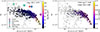 |
Fig. 9. Small grain fraction carrying MIR features (qAF) versus average interstellar radiation field intensity (⟨U⟩). Each filled circle represents a pixel of 8″ ∼ 560 pc, while the angular resolution is 25″ ∼ 1.75 kpc. Pearson correlation coefficients are listed in the top right. Left panel: Pixels colour-coded by total gas surface density ( |

Our results are consistent with previous studies of nearby galaxies (Chastenet et al. 2025; Katsioli et al. 2023, 2026). Small carbonaceous grains are efficiently photo-destroyed by hard UV photons (e.g. Luan et al. 1988, 1990; Cesarsky et al. 1996; Madden et al. 2006; Galametz et al. 2013, 2016; Galliano et al. 2018; Katsioli et al. 2023), and small grains regardless of composition are readily destroyed by SNII shock waves through kinetic sputtering (e.g. Draine & Salpeter 1979; Tielens et al. 1994; Dwek & Arendt 1992; Borkowski & Dwek 1995; Foster et al. 1993; Hu et al. 2019). In the dense molecular clouds associated with star formation8, small grains may also be efficiently depleted from the ISM via coagulation onto larger grains (e.g. Chokshi et al. 1993).
The spatially resolved qAF − ⟨U⟩ trend aligns with our integrated results, although the integrated qAF values are ∼1.6 times higher than the average pixel-based value. This difference likely reflects resolution effects, similar to those reported for other scale-dependent quantities such as the SFR (e.g. Boquien et al. 2015).
Several studies have reported a deficit of aromatic feature carriers in the diffuse ISM of nearby galaxies at sub-solar metallicities (e.g. Draine & Li 2007; Smith et al. 2007; Sandstrom et al. 2012; Whitcomb et al. 2024). This has commonly been attributed to the destruction of small grains by energetic photons in environments that are both low in metallicity and diffuse (e.g. Madden et al. 2006; Gordon et al. 2008; Egorov et al. 2023), where young stars are hotter (Massey et al. 2005) and dust attenuation is lower. To check whether this applies to M 99, we use the gas-phase metallicity measurements from De Vis et al. (2019) and Kreckel et al. (2019). Fig. 9 (right panel) shows that both qAF and ⟨U⟩ exhibit only weak correlations with metallicity, with correlation coefficients of r ∼ −0.4 for qAF and r ∼ 0.5 for ⟨U⟩. These results may partially reflect the limited coverage of our metallicity map (Fig. B.5), which only samples the central ∼8 kpc of M 99. The metallicity has typical uncertainties of ∼0.1 dex and exhibits a shallow radial gradient (Δr ∼ 0.3 dex). We conclude that radiation field intensity, rather than metallicity, is the main driver of small grain depletion in M 99, with metallicity possibly affecting only the diffuse outer ISM at low ⟨U⟩ and qAF. Extending the metallicity coverage would better constrain this relation.
4.3.3. Spatial variations of the synchrotron spectral index
The synchrotron spectral index (αsync) traces the ageing and energy loss of cosmic ray electrons (CREs) accelerated by supernova shocks and propagating through the galactic magnetic field. Other processes, such as inverse Compton scattering, ionisation, and free–free losses, can also influence αsync, particularly in dense or strongly irradiated regions (see e.g. Longair 2011; Wills et al. 1997).
We examined the variation of αsync relative to  , ΣSFR, and ⟨U⟩. Fig. 10 shows our pixel-based measurements of αsync versus ΣSFR, overlaid with the results of our integrated analysis (Sects. 4.1 and 4.2). Eight regions of enhanced star formation, highlighted by green crosses, are selected from our sSFR map (defined as ΣSFR/Σ★; see Appendix F). These measurements integrate over 25″ apertures and likely represent a mixture of emission from HII regions and the surrounding dense and diffuse ISM.
 |
Fig. 10. Synchrotron spectral index (αsync) versus SFR surface density (ΣSFR), colour-coded by total gas surface density ( |

We find strong anti-correlations between αsync and ΣSFR (r = −0.730 ± 0.003),  (r = −0.750 ± 0.004), and ⟨U⟩ (r = −0.803 ± 0.004), across the range 0.5 ≲ αsync ≲ 1.2, corresponding to the prior imposed on αsync during SED fitting (Table 6). At low SFR (ΣSFR≲ 0.01 M⊙ yr−1 kpc−2), corresponding to
  , ΣSFR ≲ 0.01 M⊙ yr−1 kpc−2 and ⟨U⟩≲7⟨U⟩⊙, αsync steepens to ≳0.9 (dark blue and black points in Fig. 10). In these lower-density regions, we expect that the injection of fresh CREs is limited and the emission is dominated by older electrons that have diffused through the ISM without significant re-acceleration.
In the central 50″ (∼3.5 kpc), where ΣSFR≳ 0.01 M⊙ yr−1 kpc−2, αsync flattens to ∼0.6, suggesting that CREs are more energetic in regions of high SFR (e.g. Condon 1992; Thompson et al. 2006). The eight candidate star-forming regions (green crosses in Fig. 10) exhibit synchrotron spectral indices of αsync ∼ 0.6 − 0.9. Most of these regions are located in areas with high ΣSFR and  , where αsync typically lies in the range ∼0.6 − 0.7. These results are in agreement with previous spatially resolved studies of radio emission in nearby galaxies (e.g. Murphy et al. 2006; Hughes et al. 2006; Basu et al. 2015; Mulcahy et al. 2016; Tabatabaei et al. 2017, 2022), where flatter non-thermal spectral indices are interpreted as a combination of recent feedback-driven injection of young CREs and limited CRE diffusion and advection.
4.3.4. Dust scaling relations
Dust is produced in the ejecta of supernovae and asymptotic giant branch, but its abundance in galaxies is strongly shaped by ISM processes: grains can grow through metal accretion in dense environments or be destroyed by shocks and stellar radiation. As a result, the dust content of galaxies is expected to scale with their stellar mass, SFR, and metallicity.
In this Sect., we examine spatially resolved scaling relations for M 99, focusing on the dust-to-stellar mass ratio (DSR =Σdust/Σ★) and dust-to-gas mass ratio (DGR =Σdust/Σgas) as functions of Σ★ and other ISM properties, including SFR, gas-phase metallicity, and molecular gas fraction, fmol (see Appendix B). The dust mass surface density (Σdust) is derived from our HerBIE fits using both the THEMIS and MBB models.
4.3.4.1. The dust-to-stellar mass ratio.
An anti-correlation between the DSR and stellar mass is well established in the literature, on integrated scales (Cortese et al. 2012; Clemens et al. 2013; Clark et al. 2015; De Vis et al. 2017a; Casasola et al. 2020; De Looze et al. 2020) and at sub-kiloparsec resolution (e.g. Viaene et al. 2014). This relation is also reproduced by theoretical models and hydrodynamical simulations (e.g. Camps et al. 2016; Calura et al. 2017; Lapi et al. 2020). The proposed explanation is that while both dust and stars are formed in star-forming regions, stellar mass accumulates continuously over time, whereas dust may be destroyed by shocks, radiation, and astration.
We find a strong anti-correlation between the DSR and Σ★ (Fig. 11, top panel) using our THEMIS fit (r = −0.909 ± 0.004, slope a ∼ −0.5) and a weaker trend for the MBB (r ∼ −0.4, a ∼ −0.11). The flatter MBB slope arises from higher inferred dust masses in dense, β > 1.79 regions. The DSR also correlates with  and ΣSFR for THEMIS (r = −0.790 ± 0.005 and r = −0.842 ± 0.005 respectively), but these correlations weaken using the MBB model (r = −0.289 ± 0.009 and r = −0.40 ± 0.01). We do not detect any significant correlation with sSFR (THEMIS: r ∼ −0.1; MBB: r ∼ 0.05).
 |
Fig. 11. Dust-to-stellar mass ratio scaling relations with stellar mass surface density (Σ★, top) and gas metallicity (bottom) in M 99. Filled circles show the THEMIS dust masses, colour-coded by molecular gas fraction (fmol); grey hexagons correspond to single-T MBB dust masses. Each symbol represents an 8″ ∼ 560 pc pixel. The angular resolution is 25″ ∼ 1.75 kpc. The bottom panel is restricted to the region covered by the metallicity map (Fig. B.5). Solid red and dashed black lines show the best-fit relations for THEMIS and MBB, respectively; green lines show correlations from Casasola et al. (2022). Red and white diamonds mark integrated values from THEMIS and MBB fits, while filled stars in the top panel indicate disc (cyan), spiral arms (blue), and centre (magenta) averages. Calibration uncertainties are indicated by grey bars near the legend. |
Our DSR-Σ★ relation is broadly consistent with the results of Casasola et al. (2022, green lines in Fig. 11), who reported a correlation with slope a = −0.56 ± 0.02 and a Pearson coefficient of r = −0.82 for a sample of 18 large, face-on spiral galaxies from DustPedia (excluding M 99). Their best-fit relation is offset by approximately 0.2 dex toward lower DSR values compared to ours (Fig. 11), but still within the reported 1σ scatter of 0.22 dex. Relative to the THEMIS-based results, the DSR-Σ★ relation inferred from the MBB modelling shows a more pronounced deviation from the trend of Casasola et al. (2022) at high stellar surface densities (Σ★ > 102 M⊙ pc−2), with offsets reaching up to 0.5 dex. However, a closer inspection of Fig. 5 in Casasola et al. (2022) suggests a possible flattening of their relation at Σ★ > 102 M⊙ pc−2 once NGC 3031 (M 81) is excluded. This brings their trend into closer agreement with our results. Overall, the remaining discrepancies in slope likely reflect intrinsic differences between the ISM properties of M 99 and those of the DustPedia galaxies analysed by Casasola et al. (2022).
Differences in normalisation of the DSR-Σ★ relation may arise from variations in stellar mass calibrations (Casasola et al. 2022 follow Querejeta et al. 2015) or dust mass estimation methods (e.g. Nersesian et al. 2019; Relaño et al. 2022, see Sect. 5.1 of Casasola et al. 2017 for details on the DustPedia dust mass estimates). Another contributing factor may be differences in data resolution and spatial sampling (Casasola et al. 2022 adopted a physical scale of 3.4 kpc per pixel), since these determine the mixing within a resolution element and hence the data’s sensitivity to local variations. The absence of a significant correlation between the DSR and sSFR suggests that the observed DSR-Σ★ anti-correlation is primarily driven by M 99’s past star formation history (SFH), rather than ongoing star formation.
The bottom panel of Fig. 11 reveals a moderate anti-correlation between the DSR and gas-phase metallicity (THEMIS: r ∼ −0.5; MBB: r ∼ −0.3). The metallicity itself correlates with the total gas surface density (r ∼ 0.6), suggesting that dense, gas-rich regions in the centre of M 99 are more metal-enriched. Thus, the observed trend between DSR and gas-phase metallicity likely reflects a depletion of dust in evolved, metal-enriched, highly irradiated environments with high Σ★. We caution that the dust masses inferred from THEMIS may be underestimated in the densest regions (Sect. 4.1).
4.3.4.2. The dust-to-gas mass ratio.
In Fig. 12, we present the pixel-by-pixel relation between the DGR and Σ★ (top panel) and gas-phase metallicity (bottom panel). The DGR inferred using THEMIS is nearly flat with Σ★ (a ∼ −0.06, r = −0.27 ± 0.03), whereas the DGR inferred from an MBB fit shows a positive trend (a ∼ 0.4, r = 0.73 ± 0.03). This discrepancy (up to 0.5 dex at high Σ★) is primarily due to the fixed β adopted by the THEMIS model. Casasola et al. (2022) found a strong positive correlation between DGR and Σ★ (a ∼ 0.37, r = 0.7), in agreement with our MBB fit, but with a ∼0.2 dex offset in normalisation. This offset may stem from differences in spatial resolution, gas and dust mass estimation methods, and the CO line transition used to trace molecular gas (Casasola et al. 2020 used CO(2–1) with fixed r21).
 |
Fig. 12. Dust-to-(total) gas mass ratio scaling relations with stellar mass surface density (Σ★, top) and gas metallicity (bottom) in M 99. Filled circles show THEMIS dust masses, colour-coded by molecular gas fraction (fmol); grey hexagons indicate single-T MBB dust masses. Each point represents an 8″ ∼ 560 pc pixel. The angular resolution is 25″ ∼ 1.75 kpc. The bottom panel covers only regions with metallicity measurements (Fig. B.5). Solid red and dashed black lines show best-fit relations for THEMIS and MBB, respectively; green lines show correlations from Casasola et al. (2022). Red and white diamonds mark integrated values for THEMIS and MBB fits. Calibration uncertainties are indicated by grey bars near the legend. |
Regions with higher Σ★ are generally expected to exhibit higher DGRs, consistent with a more metal-rich ISM resulting from prolonged, steady SFHs (e.g. De Looze et al. 2020; Galliano et al. 2021). As expected for such a steady star formation scenario, we detect no correlation between the DGR and the sSFR. We find a tight positive correlation between the DGR and the fraction of molecular gas (fmol) using the MBB model (r = 0.63 ± 0.02), while a weak anti-correlation is obtained for THEMIS (r = −0.35 ± 0.02). A flat DGR with fmol implies an almost constant fraction of dust in the neutral ISM, irrespective of whether the gas is predominantly atomic or molecular. A positive trend is more commonly reported in recent literature (Casasola et al. 2022), especially for environments with relatively high fmol (≳10%). This trend is often interpreted as evidence for dust grain growth in the ISM through accretion (typical timescales are shorter in cold and dense environments; Asano et al. 2013; Vílchez et al. 2019).
The DGR is expected to increase with metallicity since more metals are available for grain growth. Using MBB, we find a positive, superlinear trend (a ∼ 1.47, r ∼ 0.45). This is in good agreement with the relation reported by Casasola et al. (2022) (a ∼ 1.17, r = 0.7), and the full DustPedia sample of late-type galaxies (De Vis et al. 2019), as well as with the predictions of several dust evolution models (e.g. Feldmann 2015; De Vis et al. 2017b). A superlinear slope implies a significant contribution from in-situ grain growth processes that become particularly important in high-metallicity environments. Our THEMIS model instead shows a weak negative correlation between the DGR and gas-phase metallicity, likely due to the underestimation of dust masses in dense, metal-rich regions.
5. Summary
We have analysed the millimetre emission of M 99 using new 1.15 mm and 2 mm continuum maps from the NIKA2/IRAM 30 m telescope (IMEGIN Guaranteed Time Large Programme) at angular resolutions of 12″ and 18″. We combined these data with extensive ancillary multi-wavelength photometry (from UV to radio) and CO and HI line maps tracing molecular and atomic gas. We modelled the IR-to-radio SED of M 99 on both integrated and spatially resolved (1.75 kpc) scales using the hierarchical Bayesian fitting code HerBIE (Galliano 2018), decomposing dust, free-free, and synchrotron emission. We described the dust emission with the THEMIS dust model (Jones et al. 2017) and a single-T MBB. We summarise our main results and conclusions as follows.
-
We find substantial variations in the dust spectral index, β, with changes reaching up to ∼0.6 on integrated scales and up to ∼0.9 on resolved scales. The dust spectral index is systematically lower in the diffuse ISM (1.72 ± 0.09 in the disc) and increases in denser star-forming regions (1.92 ± 0.08 in spiral arms, 2.27 ± 0.09 in the centre). On kiloparsec scales, β exhibits a bimodal distribution, with peaks near 1.7 and 2.1, consistent with dust grain reprocessing, likely driven by coagulation or changes in dust grain composition. Strong correlations between β, molecular gas surface density, and the interstellar radiation field support the argument that the observed FIR slope steepening in M 99 results from dust evolution in dense or strongly irradiated environments. Accounting for variable β increases dust mass estimates by a factor of 1.6 (mean value) compared to models assuming a fixed β and up to a factor of about four in the central regions of M 99.
-
The fraction of small dust grains varies from a few percent in the galaxy centre to ∼16% in the disc, and this behaviour is anti-correlated with the average interstellar radiation field intensity. This supports the idea that small grains, sensitive to energetic UV photons, are destroyed in intense radiation fields. Gas-phase metallicity plays only a marginal role in the central 8 kpc of M 99.
-
The synchrotron spectral index varies significantly from ∼0.6 − 0.7 in central star-forming regions to ∼1.2 in the diffuse ISM, consistent with the ageing of CREs as they propagate far from the sites of star formation.
-
Correlations of DSR and DGR with stellar mass surface density, molecular gas fraction, and gas-phase metallicity are well reproduced only when allowing β to vary. Models with a fixed β can underestimate the inferred DSR and DGR by up to 0.5 dex in star-forming regions with a high molecular gas fraction.
-
These findings emphasise the need for physically motivated dust models equipped with enough flexibility to match the different ISM conditions observed in galaxies and to accurately retrieve the properties of dust grains.
Data availability
The NIKA2 images of M99, along with Tables 4, 6, 7, and 8, and the corresponding parameter and uncertainty maps presented in Sect. 4 and Appendices B and E, are available at the CDS via https://cdsarc.cds.unistra.fr/viz-bin/cat/J/A+A/709/A1
Acknowledgments
We thank the anonymous referee for the valuable feedback and insightful suggestions, which have significantly improved this manuscript. This work was funded by the P2IO LabEx (ANR-10-LABX-0038) in the framework “Investissements d’Avenir” (ANR-11-IDEX-0003-01) managed by the Agence Nationale de la Recherche (ANR, France). This work was supported by the Programme National Physique et Chimie du Milieu Interstellaire (PCMI) and the Programme National Cosmology et Galaxies (PNCG) of the CNRS/INSU with INC/INP co-funded by CEA and CNES. This work was partially funded by the Foundation Nanoscience Grenoble and the LabEx FOCUS ANR-11-LABX-0013. This work was supported by the French National Research Agency under the contracts “MKIDS”, “NIKA” and ANR-15-CE31-0017 and in the framework of the “Investissements d’avenir” programme (ANR-15-IDEX-02). This work has benefited from the support of the European Research Council Advanced Grant ORISTARS under the European Union’s Seventh Framework Programme (Grant Agreement no. 291294). This work is based in part on observations made with (i) the Spitzer Space Telescope, which was operated by the Jet Propulsion Laboratory, California Institute of Technology under a contract with NASA; (ii) Herschel, which was an ESA space observatory with science instruments provided by European-led Principal Investigator consortia and with important participation from NASA; (iii) the Galaxy Evolution Explorer (GALEX) mission; (iv) the Karl G. Jansky Very Large Array (VLA) from the National Radio Astronomy Observatory (NRAO) and the 100-m telescope of the MPIfR (Max-Planck-Institut für Radioastronomie) at Effelsberg. The NRAO is a facility of the U.S. National Science Foundation operated under cooperative agreement by Associated Universities, Inc. We would like to thank the IRAM staff for their support during the observation campaigns. The NIKA2 dilution cryostat has been designed and built at the Institut Néel. In particular, we acknowledge the crucial contribution of the Cryogenics Group, and in particular Gregory Garde, Henri Rodenas, Jean-Paul Leggeri, Philippe Camus. A.R. acknowledges financial support from the Italian Ministry of University and Research – Project Proposal CIR01_00010. E.A. acknowledges funding from the French Programme d’investissements d’avenir through the Enigmass Labex. FG acknowledges support by the French National Research Agency under the contracts WIDENING (ANR-23-ESDIR-0004) and REDEEMING (ANR-24-CE31-2530). M.M.E. acknowledges the support of the French Agence Nationale de la Recherche (ANR), under grant ANR-22-CE31-0010. M.B., A.N., and S.C.M. acknowledge support from the Flemish Fund for Scientific Research (FWO-Vlaanderen, research project G0C4723N). L.P., M.B., and I.D.L. acknowledge funding from the Belgian Science Policy Office (BELSPO) through the PRODEX project “JWST/MIRI Science exploitation” (C4000142239). S.K. acknowledges support provided by the Hellenic Foundation for Research and Innovation (HFRI) under the 3rd Call for HFRI PhD Fellowships (Fellowship Number: 5357). V.C. acknowledges funding from the INAF Mini Grant 2022 programme “Face-to-Face with the Local Universe: ISM’s Empowerment (LOCAL)” and the INAF Mini Grant 2024 programme “DustPedia meets Metal-THINGS: Dust-METAL”.
References
- Accurso, G., Saintonge, A., Catinella, B., et al. 2017, MNRAS, 470, 4750 [NASA ADS] [Google Scholar]
- Adam, R., Adane, A., Ade, P. A. R., et al. 2018, A&A, 609, A115 [NASA ADS] [CrossRef] [EDP Sciences] [Google Scholar]
- Amorín, R., Muñoz-Tuñón, C., Aguerri, J. A. L., & Planesas, P. 2016, A&A, 588, A23 [NASA ADS] [CrossRef] [EDP Sciences] [Google Scholar]
- Aniano, G., Draine, B. T., Gordon, K. D., & Sandstrom, K. 2011, PASP, 123, 1218 [Google Scholar]
- Aniano, G., Draine, B. T., Calzetti, D., et al. 2012, ApJ, 756, 138 [Google Scholar]
- Aniano, G., Draine, B. T., Hunt, L. K., et al. 2020, ApJ, 889, 150 [NASA ADS] [CrossRef] [Google Scholar]
- Asano, R. S., Takeuchi, T. T., Hirashita, H., & Inoue, A. K. 2013, EPS, 65, 213 [Google Scholar]
- Basu, A., Beck, R., Schmidt, P., & Roy, S. 2015, MNRAS, 449, 3879 [NASA ADS] [CrossRef] [Google Scholar]
- Berta, S., & Zylka, R. 2019, Welcome to the PIIC Pipelines (Pointing and Imaging In Continuum, as code by Robert Zylka), https://www.iram.fr/ gildas/dist/piic.pdf [Google Scholar]
- Bianchi, S., Casasola, V., Baes, M., et al. 2019, A&A, 631, A102 [NASA ADS] [CrossRef] [EDP Sciences] [Google Scholar]
- Bianchi, S., Casasola, V., Corbelli, E., et al. 2022, A&A, 664, A187 [NASA ADS] [CrossRef] [EDP Sciences] [Google Scholar]
- Bolatto, A. D., Wolfire, M., & Leroy, A. K. 2013, ARA&A, 51, 207 [CrossRef] [Google Scholar]
- Boquien, M., Calzetti, D., Aalto, S., et al. 2015, A&A, 578, A8 [NASA ADS] [CrossRef] [EDP Sciences] [Google Scholar]
- Borkowski, K. J., & Dwek, E. 1995, ApJ, 454, 254 [CrossRef] [Google Scholar]
- Boselli, A., Eales, S., Cortese, L., et al. 2010, PASP, 122, 261 [Google Scholar]
- Boselli, A., Fossati, M., Cuillandre, J. C., et al. 2018, A&A, 615, A114 [NASA ADS] [CrossRef] [EDP Sciences] [Google Scholar]
- Boulanger, F., Beichman, C., Desert, F. X., et al. 1988, ApJ, 332, 328 [NASA ADS] [CrossRef] [Google Scholar]
- Boulanger, F., Abergel, A., Bernard, J. P., et al. 1996, A&A, 312, 256 [Google Scholar]
- Bradley, L., Sipőcz, B., Robitaille, T., et al. 2024, https://doi.org/10.5281/zenodo.10967176 [Google Scholar]
- Calura, F., Pozzi, F., Cresci, G., et al. 2017, MNRAS, 465, 54 [Google Scholar]
- Calvo, M., Benoît, A., Catalano, A., et al. 2016, J. Low Temp. Phys., 184, 816 [CrossRef] [Google Scholar]
- Camps, P., Trayford, J. W., Baes, M., et al. 2016, MNRAS, 462, 1057 [CrossRef] [Google Scholar]
- Carpine, M. A., Ysard, N., Maury, A., & Jones, A. 2025, A&A, 698, A200 [NASA ADS] [CrossRef] [EDP Sciences] [Google Scholar]
- Casasola, V., Cassarà, L. P., Bianchi, S., et al. 2017, A&A, 605, A18 [NASA ADS] [CrossRef] [EDP Sciences] [Google Scholar]
- Casasola, V., Bianchi, S., De Vis, P., et al. 2020, A&A, 633, A100 [NASA ADS] [CrossRef] [EDP Sciences] [Google Scholar]
- Casasola, V., Bianchi, S., Magrini, L., et al. 2022, A&A, 668, A130 [NASA ADS] [CrossRef] [EDP Sciences] [Google Scholar]
- Cesarsky, D., Lequeux, J., Abergel, A., et al. 1996, A&A, 315, L309 [NASA ADS] [Google Scholar]
- Chang, Z., Zhou, J., Wilson, C. D., et al. 2020, ApJ, 900, 53 [CrossRef] [Google Scholar]
- Chastenet, J., Sandstrom, K., Chiang, I.-D., et al. 2021, ApJ, 912, 103 [NASA ADS] [CrossRef] [Google Scholar]
- Chastenet, J., Sandstrom, K., Leroy, A. K., et al. 2025, ApJS, 276, 2 [Google Scholar]
- Chastenet, J., De Looze, I., & Gordon, K. D. 2026, A&A, submitted [Google Scholar]
- Chemin, L., Huré, J.-M., Soubiran, C., et al. 2016, A&A, 588, A48 [NASA ADS] [CrossRef] [EDP Sciences] [Google Scholar]
- Chokshi, A., Tielens, A. G. G. M., & Hollenbach, D. 1993, ApJ, 407, 806 [Google Scholar]
- Chung, A., van Gorkom, J. H., Kenney, J. D. P., Crowl, H., & Vollmer, B. 2009, AJ, 138, 1741 [Google Scholar]
- Chyży, K. T., Ehle, M., & Beck, R. 2007, A&A, 474, 415 [NASA ADS] [CrossRef] [EDP Sciences] [Google Scholar]
- Clark, C. J. R., Dunne, L., Gomez, H. L., et al. 2015, MNRAS, 452, 397 [NASA ADS] [CrossRef] [Google Scholar]
- Clark, C. J. R., Verstocken, S., Bianchi, S., et al. 2018, A&A, 609, A37 [NASA ADS] [CrossRef] [EDP Sciences] [Google Scholar]
- Clemens, M. S., Negrello, M., De Zotti, G., et al. 2013, MNRAS, 433, 695 [NASA ADS] [CrossRef] [Google Scholar]
- Compiègne, M., Verstraete, L., Jones, A., et al. 2011, A&A, 525, A103 [Google Scholar]
- Condon, J. J. 1992, ARA&A, 30, 575 [Google Scholar]
- Contini, M., & Contini, T. 2003, MNRAS, 342, 299 [Google Scholar]
- Contursi, A., Lequeux, J., Cesarsky, D., et al. 2000, A&A, 362, 310 [NASA ADS] [Google Scholar]
- Cortese, L., Ciesla, L., Boselli, A., et al. 2012, A&A, 540, A52 [NASA ADS] [CrossRef] [EDP Sciences] [Google Scholar]
- Cutri, R. M., Skrutskie, M. F., van Dyk, S., et al. 2003, VizieR On-line Data Catalog: II/246 [Google Scholar]
- Dalcanton, J. J., Fouesneau, M., Hogg, D. W., et al. 2015, ApJ, 814, 3 [Google Scholar]
- Dale, D. A., Helou, G., Contursi, A., Silbermann, N. A., & Kolhatkar, S. 2001, ApJ, 549, 215 [Google Scholar]
- Davies, J. I., Baes, M., Bianchi, S., et al. 2017, PASP, 129, 044102 [NASA ADS] [CrossRef] [Google Scholar]
- De Looze, I., Lamperti, I., Saintonge, A., et al. 2020, MNRAS, 496, 3668 [NASA ADS] [CrossRef] [Google Scholar]
- de Vaucouleurs, G., de Vaucouleurs, A., Corwin, H. G., Jr., et al. 1991, Third Reference Catalogue of Bright Galaxies (New York, NY, USA: Springer) [Google Scholar]
- De Vis, P., Dunne, L., Maddox, S., et al. 2017a, MNRAS, 464, 4680 [NASA ADS] [CrossRef] [Google Scholar]
- De Vis, P., Gomez, H. L., Schofield, S. P., et al. 2017b, MNRAS, 471, 1743 [Google Scholar]
- De Vis, P., Jones, A., Viaene, S., et al. 2019, A&A, 623, A5 [NASA ADS] [CrossRef] [EDP Sciences] [Google Scholar]
- Demyk, K., Gromov, V., Meny, C., et al. 2022, A&A, 666, A192 [NASA ADS] [CrossRef] [EDP Sciences] [Google Scholar]
- Dignan, A., Murphy, E. J., Mason, B., et al. 2025, ApJ, 988, 216 [Google Scholar]
- Drabek, E., Hatchell, J., Friberg, P., et al. 2012, MNRAS, 426, 23 [Google Scholar]
- Draine, B. T., & Li, A. 2007, ApJ, 657, 810 [CrossRef] [Google Scholar]
- Draine, B. T., & Salpeter, E. E. 1979, ApJ, 231, 438 [Google Scholar]
- Duc, P.-A., & Bournaud, F. 2008, ApJ, 673, 787 [NASA ADS] [CrossRef] [Google Scholar]
- Dwek, E., & Arendt, R. G. 1992, ARA&A, 30, 11 [Google Scholar]
- Egorov, O. V., Kreckel, K., Sandstrom, K. M., et al. 2023, ApJ, 944, L16 [NASA ADS] [CrossRef] [Google Scholar]
- Ejlali, G., Tabatabaei, F. S., Roussel, H., et al. 2025, A&A, 693, A88 [NASA ADS] [CrossRef] [EDP Sciences] [Google Scholar]
- Feldmann, R. 2015, MNRAS, 449, 3274 [NASA ADS] [CrossRef] [Google Scholar]
- Fletcher, A., Beck, R., Shukurov, A., Berkhuijsen, E. M., & Horellou, C. 2011, MNRAS, 412, 2396 [CrossRef] [Google Scholar]
- Foster, S. M., Dwek, E., Raymond, J., & Vancura, O. 1993, Am. Astron. Soc. Meet. Abstr., 183, 14.04 [Google Scholar]
- Gajović, L., Adebahr, B., Basu, A., et al. 2024, A&A, 689, A68 [NASA ADS] [CrossRef] [EDP Sciences] [Google Scholar]
- Galametz, M., Hony, S., Galliano, F., et al. 2013, MNRAS, 431, 1596 [NASA ADS] [CrossRef] [Google Scholar]
- Galametz, M., Hony, S., Albrecht, M., et al. 2016, MNRAS, 456, 1767 [NASA ADS] [CrossRef] [Google Scholar]
- Galliano, F. 2018, MNRAS, 476, 1445 [NASA ADS] [CrossRef] [Google Scholar]
- Galliano, F. 2022, Habilitation Thesis, 1 [Google Scholar]
- Galliano, F., Hony, S., Bernard, J. P., et al. 2011, A&A, 536, A88 [NASA ADS] [CrossRef] [EDP Sciences] [Google Scholar]
- Galliano, F., Galametz, M., & Jones, A. P. 2018, ARA&A, 56, 673 [Google Scholar]
- Galliano, F., Nersesian, A., Bianchi, S., et al. 2021, A&A, 649, A18 [EDP Sciences] [Google Scholar]
- Geman, S., & Geman, D. 1984, IEEE Trans. Pattern Anal. Mach. Intell., PAMI-6, 721 [CrossRef] [Google Scholar]
- Genzel, R., Tacconi, L. J., Combes, F., et al. 2012, ApJ, 746, 69 [Google Scholar]
- Gordon, K. D., Engelbracht, C. W., Rieke, G. H., et al. 2008, ApJ, 682, 336 [NASA ADS] [CrossRef] [Google Scholar]
- Hartigan, J. A., & Hartigan, P. M. 1985, Ann. Stat., 13, 70 [Google Scholar]
- Haynes, M. P., Giovanelli, R., Kent, B. R., et al. 2018, ApJ, 861, 49 [Google Scholar]
- Holwerda, B. W., Bianchi, S., Böker, T., et al. 2012, A&A, 541, L5 [NASA ADS] [CrossRef] [EDP Sciences] [Google Scholar]
- Hu, C.-Y., Zhukovska, S., Somerville, R. S., & Naab, T. 2019, MNRAS, 487, 3252 [NASA ADS] [CrossRef] [Google Scholar]
- Hughes, A., Wong, T., Ekers, R., et al. 2006, MNRAS, 370, 363 [NASA ADS] [CrossRef] [Google Scholar]
- IRAC Instrument& Instrument Support Teams. 2021, IRAC Instrument Handbook, https://irsa.ipac.caltech.edu/data/SPITZER/docs/irac/iracinstrumenthandbook/ [Google Scholar]
- Jiménez-Donaire, M. J., Bigiel, F., Leroy, A. K., et al. 2019, ApJ, 880, 127 [CrossRef] [Google Scholar]
- Jones, A. P., Fanciullo, L., Köhler, M., et al. 2013, A&A, 558, A62 [NASA ADS] [CrossRef] [EDP Sciences] [Google Scholar]
- Jones, A. P., Köhler, M., Ysard, N., Bocchio, M., & Verstraete, L. 2017, A&A, 602, A46 [NASA ADS] [CrossRef] [EDP Sciences] [Google Scholar]
- Katsioli, S., Xilouris, E. M., Kramer, C., et al. 2023, A&A, 679, A7 [CrossRef] [EDP Sciences] [Google Scholar]
- Katsioli, S., Xilouris, E. M., Galliano, F., et al. 2026, MNRAS, 546, stag083 [Google Scholar]
- Keenan, R. P., Marrone, D. P., & Keating, G. K. 2025, ApJ, 979, 228 [Google Scholar]
- Kelly, B. C., Shetty, R., Stutz, A. M., et al. 2012, ApJ, 752, 55 [NASA ADS] [CrossRef] [Google Scholar]
- Kennicutt, R. C., Calzetti, D., Aniano, G., et al. 2011, PASP, 123, 1347 [Google Scholar]
- Köhler, M., Guillet, V., & Jones, A. 2011, A&A, 528, A96 [NASA ADS] [CrossRef] [EDP Sciences] [Google Scholar]
- Köhler, M., Jones, A., & Ysard, N. 2014, A&A, 565, L9 [NASA ADS] [CrossRef] [EDP Sciences] [Google Scholar]
- Köhler, M., Ysard, N., & Jones, A. P. 2015, A&A, 579, A15 [NASA ADS] [CrossRef] [EDP Sciences] [Google Scholar]
- Kreckel, K., Ho, I. T., Blanc, G. A., et al. 2019, ApJ, 887, 80 [NASA ADS] [CrossRef] [Google Scholar]
- Kroupa, P. 2001, MNRAS, 322, 231 [NASA ADS] [CrossRef] [Google Scholar]
- Lamperti, I., Saintonge, A., De Looze, I., et al. 2019, MNRAS, 489, 4389 [Google Scholar]
- Lapi, A., Pantoni, L., Boco, L., & Danese, L. 2020, ApJ, 897, 81 [NASA ADS] [CrossRef] [Google Scholar]
- Leroy, A. K., Walter, F., Brinks, E., et al. 2008, AJ, 136, 2782 [Google Scholar]
- Leroy, A. K., Walter, F., Bigiel, F., et al. 2009, AJ, 137, 4670 [Google Scholar]
- Leroy, A. K., Schinnerer, E., Hughes, A., et al. 2021, ApJS, 257, 43 [NASA ADS] [CrossRef] [Google Scholar]
- Li, A. 2007, ASP Conf. Ser., 373, 561 [Google Scholar]
- Linden, S. T., Murphy, E. J., Dong, D., et al. 2020, ApJS, 248, 25 [NASA ADS] [CrossRef] [Google Scholar]
- Longair, M. S. 2011, High Energy Astrophysics (Cambridge University Press) [Google Scholar]
- Luan, L., Werner, M. W., Sellgren, K., & Heiles, C. 1988, BAAS, 20, 983 [Google Scholar]
- Luan, L., Werner, M. W., Heiles, C., & Sellgren, K. 1990, NASA Conf. Publ., 3084, 108 [Google Scholar]
- Madden, S. C., Galliano, F., Jones, A. P., & Sauvage, M. 2006, A&A, 446, 877 [NASA ADS] [CrossRef] [EDP Sciences] [Google Scholar]
- Marsh, K. A., Whitworth, A. P., Lomax, O., et al. 2017, MNRAS, 471, 2730 [Google Scholar]
- Martin, D. C., Fanson, J., Schiminovich, D., et al. 2005, ApJ, 619, L1 [Google Scholar]
- Massey, P., Puls, J., Pauldrach, A. W. A., et al. 2005, ApJ, 627, 477 [NASA ADS] [CrossRef] [Google Scholar]
- Mathis, J. S., Mezger, P. G., & Panagia, N. 1983, A&A, 128, 212 [NASA ADS] [Google Scholar]
- Mulcahy, D. D., Fletcher, A., Beck, R., Mitra, D., & Scaife, A. M. M. 2016, A&A, 592, A123 [NASA ADS] [CrossRef] [EDP Sciences] [Google Scholar]
- Murphy, E. J., Helou, G., Braun, R., et al. 2006, ApJ, 651, L111 [NASA ADS] [CrossRef] [Google Scholar]
- Narayanan, D., Krumholz, M. R., Ostriker, E. C., & Hernquist, L. 2012, MNRAS, 421, 3127 [NASA ADS] [CrossRef] [Google Scholar]
- Nersesian, A., Xilouris, E. M., Bianchi, S., et al. 2019, A&A, 624, A80 [NASA ADS] [CrossRef] [EDP Sciences] [Google Scholar]
- Ormel, C. W., Min, M., Tielens, A. G. G. M., Dominik, C., & Paszun, D. 2011, A&A, 532, A43 [NASA ADS] [CrossRef] [EDP Sciences] [Google Scholar]
- Ossenkopf, V., & Henning, T. 1994, A&A, 291, 943 [NASA ADS] [Google Scholar]
- Paradis, D., Mény, C., Noriega-Crespo, A., et al. 2024, A&A, 691, A241 [NASA ADS] [CrossRef] [EDP Sciences] [Google Scholar]
- Park, H.-J., Battisti, A. J., Wisnioski, E., et al. 2024, MNRAS, 535, 729 [Google Scholar]
- Pattle, K., Gear, W., & Wilson, C. D. 2023, MNRAS, 522, 2339 [Google Scholar]
- Perley, R. A., & Butler, B. J. 2015, Am. Astron. Soc. Meet. Abstr., 225, 311.06 [Google Scholar]
- Perley, R. A., Chandler, C. J., Butler, B. J., & Wrobel, J. M. 2011, ApJ, 739, L1 [Google Scholar]
- Perotto, L., Ponthieu, N., Macías-Pérez, J. F., et al. 2020, A&A, 637, A71 [NASA ADS] [CrossRef] [EDP Sciences] [Google Scholar]
- Pilbratt, G. L., Riedinger, J. R., Passvogel, T., et al. 2010, A&A, 518, L1 [NASA ADS] [CrossRef] [EDP Sciences] [Google Scholar]
- Pilyugin, L. S., & Grebel, E. K. 2016, MNRAS, 457, 3678 [NASA ADS] [CrossRef] [Google Scholar]
- Poznanski, D., Butler, N., Filippenko, A. V., et al. 2009, ApJ, 694, 1067 [NASA ADS] [CrossRef] [Google Scholar]
- Puget, J. L., & Leger, A. 1989, ARA&A, 27, 161 [NASA ADS] [CrossRef] [Google Scholar]
- Querejeta, M., Meidt, S. E., Schinnerer, E., et al. 2015, ApJS, 219, 5 [NASA ADS] [CrossRef] [Google Scholar]
- Querejeta, M., Schinnerer, E., Meidt, S., et al. 2021, A&A, 656, A133 [NASA ADS] [CrossRef] [EDP Sciences] [Google Scholar]
- Relaño, M., De Looze, I., Saintonge, A., et al. 2022, MNRAS, 515, 5306 [CrossRef] [Google Scholar]
- Rémy-Ruyer, A., Madden, S. C., Galliano, F., et al. 2013, A&A, 557, A95 [Google Scholar]
- Roussel, H. 2013, PASP, 125, 1126 [Google Scholar]
- Sadavoy, S. I., Di Francesco, J., Johnstone, D., et al. 2013, ApJ, 767, 126 [Google Scholar]
- Salvestrini, F., Bianchi, S., & Corbelli, E. 2025, A&A, 699, A346 [NASA ADS] [CrossRef] [EDP Sciences] [Google Scholar]
- Sandstrom, K. M., Bolatto, A. D., Bot, C., et al. 2012, ApJ, 744, 20 [CrossRef] [Google Scholar]
- Schruba, A., Leroy, A. K., Walter, F., et al. 2011, AJ, 142, 37 [NASA ADS] [CrossRef] [Google Scholar]
- Shetty, R., Kauffmann, J., Schnee, S., & Goodman, A. A. 2009, ApJ, 696, 676 [NASA ADS] [CrossRef] [Google Scholar]
- Smith, J. D. T., Draine, B. T., Dale, D. A., et al. 2007, ApJ, 656, 770 [Google Scholar]
- Smith, M. W. L., Eales, S. A., De Looze, I., et al. 2016, MNRAS, 462, 331 [NASA ADS] [CrossRef] [Google Scholar]
- Smith, M. W. L., Eales, S. A., Williams, T. G., et al. 2021, ApJS, 257, 52 [Google Scholar]
- Soria, R., & Wong, D. S. 2006, MNRAS, 372, 1531 [Google Scholar]
- Tabatabaei, F. S., Schinnerer, E., Murphy, E. J., et al. 2013, A&A, 552, A19 [NASA ADS] [CrossRef] [EDP Sciences] [Google Scholar]
- Tabatabaei, F. S., Braine, J., Xilouris, E. M., et al. 2014, A&A, 561, A95 [NASA ADS] [CrossRef] [EDP Sciences] [Google Scholar]
- Tabatabaei, F. S., Schinnerer, E., Krause, M., et al. 2017, ApJ, 836, 185 [Google Scholar]
- Tabatabaei, F. S., Cotton, W., Schinnerer, E., et al. 2022, MNRAS, 517, 2990 [NASA ADS] [CrossRef] [Google Scholar]
- Tailor, V., Casasola, V., Pozzi, F., et al. 2025, A&A, 701, A74 [NASA ADS] [CrossRef] [EDP Sciences] [Google Scholar]
- Thompson, T. A., Quataert, E., Waxman, E., Murray, N., & Martin, C. L. 2006, ApJ, 645, 186 [NASA ADS] [CrossRef] [Google Scholar]
- Tielens, A. G. G. M., McKee, C. F., Seab, C. G., & Hollenbach, D. J. 1994, ApJ, 431, 321 [NASA ADS] [CrossRef] [Google Scholar]
- Viaene, S., Fritz, J., Baes, M., et al. 2014, A&A, 567, A71 [NASA ADS] [CrossRef] [EDP Sciences] [Google Scholar]
- Vílchez, J. M., Relaño, M., Kennicutt, R., et al. 2019, MNRAS, 483, 4968 [CrossRef] [Google Scholar]
- Werner, M. W., Roellig, T. L., Low, F. J., et al. 2004, ApJS, 154, 1 [NASA ADS] [CrossRef] [Google Scholar]
- Whitcomb, C. M., Smith, J. D. T., Sandstrom, K., et al. 2024, ApJ, 974, 20 [Google Scholar]
- Whittet, D. C. B. 2022, Dust in the Galactic Environment (Third Edition) (Bristol: IOP Publishing) [Google Scholar]
- Wielebinski, R., Junkes, N., & Grahl, B. H. 2011, J. Astron. Hist. Heritage, 14, 3 [Google Scholar]
- Wills, K. A., Pedlar, A., Muxlow, T. W. B., & Wilkinson, P. N. 1997, MNRAS, 291, 517 [NASA ADS] [CrossRef] [Google Scholar]
- Yoon, J. H., Martin, C. L., Veilleux, S., et al. 2021, MNRAS, 502, 969 [NASA ADS] [CrossRef] [Google Scholar]
- Ysard, N., Köhler, M., Jones, A., et al. 2016, A&A, 588, A44 [NASA ADS] [CrossRef] [EDP Sciences] [Google Scholar]
- Ysard, N., Jones, A. P., Demyk, K., Boutéraon, T., & Koehler, M. 2018, A&A, 617, A124 [NASA ADS] [CrossRef] [EDP Sciences] [Google Scholar]
- Ysard, N., Jones, A. P., Guillet, V., et al. 2024, A&A, 684, A34 [NASA ADS] [CrossRef] [EDP Sciences] [Google Scholar]
- Zylka, R. 2013, Astrophysics Source Code Library [record ascl:1303.011] [Google Scholar]
Publicly available on GitLab: https://gitlab.com/imegin/hip
With qPAH = 0.45 × qAF (Galliano et al. 2021).
A Hartigan’s dip test with N = 100 gives a dip statistic of 0.12 and a p-value of 0.045. A dip value ≳0.03 − 0.05 with p-value < 0.05 is typically considered strong evidence against unimodality (Hartigan & Hartigan 1985).
All reported correlations in this work are statistically significant, with p-values ≪10−3. If provided, the uncertainty on the Pearson correlation coefficient r is estimated using the MCMC method within the hierarchical Bayesian framework.
Silicate grains with no or thinner carbonaceous mantles have steeper FIR emissivity if exposed to the same ISRF (Köhler et al. 2014).
Spatial scales of ∼1.75 kpc, corresponding to our working resolution, encompass both dense molecular clouds and HII regions.
Because their size (≲100 pc) is much smaller than our 1.75 kpc resolution, molecular clouds are blended with the surrounding irradiated medium and do not appear as a distinct low-⟨U⟩ component.
The CO-to-H2 conversion factor has been suggested to be strongly dependent on the gas-phase metallicity (e.g. Genzel et al. 2012; Schruba et al. 2011; Amorín et al. 2016; Accurso et al. 2017). Many works in the literature showed that this dependence, if taken into account, can lead to systematically larger conversion factors, up to a factor of 3 (e.g. Casasola et al. 2017; Salvestrini et al. 2025). However, this systematics is consistent, within 2σ, with the uncertainty driven by the variety of gas-phase metallicity calibrations (i.e. ∼0.2 dex; Amorín et al. 2016).
For J magnitudes < 13.5, < 14, < 15.5, < 16, < 18, < 40 we use, in the order, the following factors: 4.6, 3.0, 2.1, 1.4, 1.15, 0.7.
Error maps quantify the instrumental noise.
Appendix A: Millimetre observations of M 99 with NIKA2
In this Appendix, we examine the mm morphology of M 99 and assess and quantify the effects of large-scale filtering.
A.1. Millimetre morphology
Figure A.1 compares the morphology observed with NIKA2 and SPIRE 250 μm. Notably, the angular resolution of the SPIRE 250 μm data (18″) matches that of NIKA2 at 2 mm. The NIKA2 2.5σ contour (in light pink) closely follows the SPIRE 250 μm 15σ contour, while higher NIKA2 significance levels (5σ and 7.5σ; darker pink) lie well within the 55σ SPIRE contour. Overall, the millimetre morphology traced by NIKA2 aligns well with the FIR morphology from SPIRE, within NIKA2’s detection limits, possibly reflecting an intrinsic compactness of M 99 at millimetre wavelengths.
 |
Fig. A.1. Scanam_nika filled contours of M 99 (shades of pink; levels of [2.5, 5, 7.5]×σ) at 1.15 mm (top) and at 2 mm (bottom) overlaid with SPIRE 250 μm contours (white solid lines; levels of [5, 15, 35, 55]×σ). |
A.2. Large-scale filtering
As is the case for other ground-based millimetre observatories (e.g. SCUBA2 on the JCMT; Sadavoy et al. 2013; Smith et al. 2021; Pattle et al. 2023), NIKA2 observations of extended sources are affected by spatial filtering on large angular scales. This filtering leads to a partial loss of large-scale emission, arising from the combined effects of instrumental and atmospheric noise and the scanning strategy adopted for mapping extended regions.
The Scanam_nika data-processing pipeline is specifically designed to mitigate this effect, as described in Appendix A.1 of Ejlali et al. (2025). Its core principle is to fully exploit the observational redundancy, with each position within the nominal sky coverage being sampled multiple times by different detectors under varying atmospheric conditions, while making minimal assumptions about the noise properties. The noise is decomposed into high- and low-frequency components, following the methodology detailed in Appendix A.2 of Ejlali et al. (2025). Further details will be presented in the forthcoming IMEGIN catalogue paper (Ejlali et al., in prep.).
We computed the transfer functions of the NIKA2 maps of M 99 using the SPIRE 250 μm image, i.e. our morphological reference. We simulated the SPIRE 250 map through the Scanam_nika pipeline after injecting the NIKA2 total noise at 1.15 mm and 2 mm, following the procedure described in Ejlali et al. (2025, Appendix A.3). Comparing the simulated output maps with the original input maps directly yields the spatially resolved transfer functions. The transfer functions are presented in bins of S/N ratio (Fig. A.2), with the low-S/N tail corresponding to the most diffuse emission at large scales. At 1.15 mm, the transfer function reaches approximately 95% flux recovery up to the 3σ bin. At 2 mm, the recovered flux is about 90% in the 3σ bin, increases to nearly 100% at 7σ, and remains flat at higher S/N ratios.
 |
Fig. A.2. Transfer functions from the SPIRE 250 μm simulations binned as a function of S/N, with 1.15 mm (top panel) and 2 mm (bottom panel) total noise (solid black lines; grey shaded areas show the associated uncertainties), i.e. the sum of high frequency (HF) and low frequency (LF) noise. The noise standard deviation σHF is from a simulation including only high-frequency noise (dashed line). The red curve and red shaded area show the cumulative fraction of the flux that is recovered and the associated uncertainties. |
Given the relatively minor filtering effects within the 3σ threshold, we incorporated this contribution into the overall uncertainty budget. This additional uncertainty was treated as a systematic error and combined in quadrature with the statistical uncertainties. The relative uncertainty introduced by large-scale filtering in the NIKA2 maps was estimated from the flux difference between the original and simulated data. On an integrated scale (within the ellipse used for integrated photometry; Fig. C.4), these relative uncertainties amount to ∼5% at 1.15 mm and 15% at 2 mm. When considering distinct morphological components, the relative uncertainties at 1.15 mm are 5% for the spiral arms and disc and 1% for the centre. At 2 mm, the uncertainties are 7% for the spiral arms, 16% for the disc, and 2% for the centre.
The pixel-scale uncertainty was quantified using the following procedure. We constructed the map (Fig. A.3) of the relative difference between the original and the simulated SPIRE 250 μm image, i.e. (Sorig − Ssimu)/Sorig, within the 3σ level measured on the simulated map (i.e. 3σsimu; see Fig. A.2). Then, we computed the distribution of the relative difference (figure insets). The spread of this distribution, which we quantified using the median absolute deviation (MAD), provides an estimate of the flux recovery accuracy within 3σsimu. The MAD is approximately 10% at both 1.15 mm and 2 mm. The NIKA2 flux densities corresponding to the 3σ level of the simulated maps are 0.24 mJy at 1.15 mm and 0.022 mJy at 2 mm (orange solid contours in Fig. A.3). These values imply flat noise levels of 0.024 mJy at 1.15 mm and 0.0022 mJy at 2 mm. This flat noise component was added in quadrature, on a pixel-by-pixel basis, to the NIKA2 RMS maps.
 |
Fig. A.3. Relative differences between the original and simulated SPIRE 250 μm maps, using 1.15 mm noise and mask (top) and 2 mm noise and mask (bottom). All images are degraded and resampled to the SPIRE 350 μm resolution. The 3σ level from the simulated maps (3σsimu) is shown in black, with corresponding NIKA2 contours in orange. Cyan contours show the original SPIRE 250 μm emission (as in Fig. A.1). Figure insets display the distribution of relative differences (ΔS), with MAD values of 0.06 (1.15 mm) and 0.07 (2 mm), both approximated to 0.1. |
A.3. Comparison with Planck observations
To further validate the NIKA2 maps produced with the Scanam_nika software, we compared the integrated NIKA2 fluxes with independent measurements. Specifically, we used the corresponding flux densities derived from Planck, as described below.
We modelled and subtracted the sky emission from Planck images, dominated by the CMB, using HIP (see Appendix C), as displayed in Fig. A.4. Since M 99 is unresolved and the coarse pixel size causes the galaxy’s emission to spread into adjacent pixels, we measured the integrated flux within a circular aperture, with a radius matching the Planck beam (r = 300″; solid yellow line in the top panels of Figs. A.4). The resulting integrated flux of M 99 at 1.38 mm, measured on the sky-subtracted Planck map, is 0.37 ± 0.07 Jy (versus the 0.52 ± 0.06 Jy measured on the original map). At 2 mm, the integrated flux we measured on the original Planck map is −0.07 ± 0.04 Jy. After correcting for the background emission, we measured an integrated flux of 0.03 ± 0.05 Jy, which is consistent with 0. Thus, Planck does not detect M 99 at 2 mm.
 |
Fig. A.4. Original Planck maps of M 99 at 1.38 mm and 2.1 mm (top panels), overlaid with the circles used for computing the growth curve. The modelled sky maps are shown in the central panels. Bottom panels show the growth curves computed on the original Planck maps (red solid lines) and on the sky-subtracted maps (green solid lines). The blue-filled circles indicate the value of the integrated flux, corresponding to the yellow circles in the top panels (r = 300″). |
Since Planck and NIKA2 have different filter shapes and central wavelengths, we performed a ‘colour correction’, which implies the assumption of a reference model. Dust emission at mm wavelengths is reasonably well described by the Rayleigh-Jeans approximation for Tdust ≳ 20 K; thus a sensible reference model is
 (A.1)
(A.1)
where β ∼ 2 and SRJ is the observed flux in the Rayleigh-Jeans tail. We used HerBIE’s synthetic photometry module (Galliano 2018) for integrating, in the range 0.3 mm < λ < 3 mm, NIKA2 and Planck bandpasses with central wavelengths 1.15 mm and 1.38 mm. The following expression gives the ‘colour correction’:
 (A.2)
(A.2)
which implies
 (A.3)
(A.3)
The term SC represents the colour-corrected Planck flux at λ = 1.15 mm, i.e. the total flux we expect to measure on the NIKA2 1.15 mm map of M 99, given the flux we measure on the Planck 1.38 mm map. This value is consistent with the Scanam_nika integrated flux, i.e. 0.65 ± 0.04 Jy.
Appendix B: Ancillary maps
This Appendix outlines the methodology used to derive the ancillary maps.
B.1. Stellar mass surface density
We derived the stellar mass surface density map of M 99 using the calibration by Leroy et al. (2008, Eq. C1), under the assumption of a Kroupa (2001) Initial Mass Function (IMF). This calibration is based on Spitzer/IRAC 3.6 μm surface brightness and reads
 (B.1)
(B.1)
where i is the galaxy inclination and I3.6 is the Spitzer/IRAC surface brightness at 3.6 μm.
The calibration relies on an empirical conversion from 3.6 μm emission to K-band intensity, assuming a standard mass-to-light ratio of 0.5 M⊙/L⊙ typical of star-forming galaxies. This assumption dominates the calibration uncertainty, with ∼0.1 dex scatter due to variations in SFH, metallicity, and IMF (Leroy et al. 2008).
In Fig. B.1 we show the resulting stellar mass surface density map of M 99. The associated uncertainties were estimated via the MC approach with 103 iterations. From our map we derived a total stellar mass of (4 ± 1)×1010 M⊙ for M 99, consistent with literature values (e.g. Chemin et al. 2016; Leroy et al. 2021).
 |
Fig. B.1. Stellar mass surface density of M 99. The map is convolved to match NIKA2 angular resolution at 2 mm and pixel size. |
B.2. Star formation rate surface density
We derived the SFR surface density of M 99 using the calibration by Leroy et al. (2008, Eq. D1), with 1σ scatter of 0.22 dex:
 (B.2)
(B.2)
where IFUV and I24, μm are the GALEX FUV and Spitzer/MIPS 24 μm surface brightnesses, respectively (Table 2), and i is the inclination angle in radians (Table 1).
We corrected the GALEX FUV and Spitzer/MIPS 24 μm maps for emission from evolved stars using the Spitzer/IRAC 3.6 μm map (Table 2), following the method of Pattle et al. (2023):
![Mathematical equation: $$ \begin{aligned} \begin{array}{cc} I_{\rm FUV, \,SF} = I_{\rm FUV} - 10^{-3}\times I_{\rm 3.6\, \mu m} \quad [\mathrm{MJy\,sr^{-1}}]\\ I_{\rm 24 \,\mu m, \,SF} = I_{\rm 24\, \mu m} - 0.1\times I_{\rm 3.6\, \mu m} \quad [\mathrm{MJy\,sr^{-1}}].\\ \end{array} \end{aligned} $$](/articles/aa/full_html/2026/05/aa57583-25/aa57583-25-eq25.gif) (B.3)
(B.3)
Figure B.2 shows the resulting SFR surface density map. Uncertainties from the intensity maps and the intrinsic scatter of the calibrations were propagated via a Monte Carlo method with NMC = 103 iterations.
 |
Fig. B.2. Star formation rate density of M 99. The map is shown at 18″ angular resolution and 3″ pixel size, matching NIKA2 at 2 mm. |
From our map we measured a total SFR of 3 M⊙ yr−1, with a 3σ confidence interval of [0.66, 13.7] M⊙ yr−1. This value agrees with estimates from the literature (e.g. Tabatabaei et al. 2017; Leroy et al. 2021), despite differences in the adopted calibrations (e.g. Boselli et al. 2018).
B.3. Atomic and molecular gas masses
We derived the atomic gas mass surface density (ΣHI) from the 21 cm line intensity map (I21 cm) of M 99 (Table 3), by Chung et al. (2009). We assumed optically thin HI emission following standard practice (e.g. Schruba et al. 2011; Casasola et al. 2017)
 (B.4)
(B.4)
where i is the inclination angle of the galaxy. The associated uncertainty ranges between approximately 0.1 and 0.15 dex (Aniano et al. 2020; Casasola et al. 2020, 2022).
Figure B.3 presents the resulting HI mass surface density map at the original angular resolution of 30″. From our map we found a total atomic hydrogen mass of MHI = (7 ± 1)×109 M⊙, in agreement with the literature (e.g. Chemin et al. 2016; Haynes et al. 2018).
 |
Fig. B.3. Atomic gas mass surface density of M 99. Spatial resolution and pixel size are the same as the original HI map, i.e. 30″ and 5″, respectively. |
We derived the molecular gas mass surface density ( ) using the CO(1–0) line intensity map by the EMPIRE programme (Jiménez-Donaire et al. 2019, Table 3). We adopted a constant CO-to-H2 conversion factor9, i.e. XCO = 2.0 × 1020 cm−2 (K km s−1)−1, following Bolatto et al. (2013). Specifically, XCO= N(H2)/ICO, where N(H2) is the molecular gas column density in cm−2, and ICO is the CO line intensity in K km s−1. This value corresponds to αCO = 3.2 M⊙ pc−2 (K km s−1)−1 (Narayanan et al. 2012), where αCO = M(H2)/L(CO), with M(H2) being the H2 mass in M⊙ and L(CO) the luminosity of the CO line in K km s−1 pc2. Ultimately, we used the calibration by Schruba et al. (2011, see also Casasola et al. (2017)):
 (B.5)
(B.5)
where i is the inclination angle of the galaxy (Table 1). The associated scatter is ∼0.3 dex, mostly due to the uncertainties on the constant CO-to-H2 conversion factor (Bolatto et al. 2013).
In Fig.B.4 we show the surface density map of the molecular gas in M 99 at native angular resolution of 25.6″. We measured a total molecular gas mass of MH2 = (6 ± 2)×109 M⊙, consistent with the literature (e.g. Chemin et al. 2016; Casasola et al. 2020).
 |
Fig. B.4. Molecular gas surface density map of M 99. Spatial resolution and pixel size are the same as the original CO(1–0) map, i.e. 25.6″ and 4″, respectively. |
In addition, we computed the molecular gas surface density of M 99 at an improved angular resolution of 18″, matching that of the NIKA2 2 mm map, using the CO(2–1) intensity map from Jiménez-Donaire et al. (2019, Table 3). The CO(2–1)/CO(1–0) ratio, r21, was derived pixel-by-pixel at the native CO(1–0) resolution (25″), yielding a mean value of ⟨r21⟩ = 0.7 ± 0.2 with no significant spatial variation, consistent with MW-like galaxies (e.g. Keenan et al. 2025). The CO(2–1) map was then convolved to 25″ to match CO(1–0), and Eq. (B.5) was applied to derive the molecular gas surface density.
Both calibrations, Eqs. (B.4) and (B.5), include a factor of 1.36 to account for helium and heavier elements. We propagated uncertainties through the MC approach with NMC = 103 iterations, incorporating the intrinsic scatter of the calibrations.
B.4. Metallicity
We constructed the gas-phase metallicity map of M 99 by leveraging recent PHANGS-MUSE measurements (Kreckel et al. 2019) combined with the compilation of approximately 1900 HII regions from the DustPedia collaboration (De Vis et al. 2019). Metallicities were calibrated using the S calibration of Pilyugin & Grebel (2016).
Metallicity measurements are typically obtained within 1″ apertures, well below our working angular resolution (25″) and pixel size 6″. Using the SPIRE 250 μm map as a reference, we averaged all metallicity measurements that fall within each 6″ pixel. Fig. B.5 shows the resulting metallicity map of M 99. The associated uncertainties mostly range between 0.01 and 0.05 in units of 12 + log(O/H), corresponding to ∼0.1 dex.
 |
Fig. B.5. Metallicity map of M 99, overlaid with SPIRE 250 μm contours (cyan solid lines; levels of [5, 15, 55, 100]×σ). Spatial resolution and pixel size are the same as the SPIRE 250 μm map. |
Appendix C: Homogenisation for IMEGIN Photometry post-processing pipeline (HIP)
The Homogenisation for IMEGIN Photometry post-processing pipeline (HIP) performs multiple steps to remove astrophysical and artificial contamination from the images, homogenise the dataset, and propagate uncertainties. HIP offers flexible control over the selection and sequencing of these steps, as well as the option to enable or disable uncertainty propagation. In the following sections, we detail each step we executed for the processing of M 99, following the order applied.
C.1. Foreground stars
The HIP pipeline identifies foreground stars near the target galaxy by querying the point source catalogue of Cutri et al. (2003). The stars are selected to have J < 40 mag. HIP masks each star using a circular region with a default radius twice the map’s spatial resolution (FWHM), accounting for the point source emission spreading into adjacent pixels. Additionally, it applies a magnitude-dependent scaling factor to address pixel saturation and bleeding effects10.
We ran this step for wavelengths λ < 24 μm, where stellar emission dominates. Fig. C.1 illustrates the GALEX NUV map of M 99 after masking the brightest foreground stars with HIP.
 |
Fig. C.1. GALEX NUV map of M 99 (in log scale and at native angular resolution, i.e. 5.3″) where the emission coming from the brightest foreground stars is masked. The position and the geometry of M 99 are highlighted with a white ellipse, defined in Appendix C.5. |
C.2. Sky subtraction
In HIP the large-scale sky structures are modelled using the Background2D class from Photutils11 (Bradley et al. 2024). HIP divides the input map into a square mesh, with each cell size defined as an integer multiple of the map’s spatial resolution, in order to capture local variations of the sky. The default multiplier is 10 and the total number of cells follows accordingly. For each cell, it calculates the mean or median sky emission (depending on the number of pixels), after applying a 3σ threshold to reject outliers. Then, it performs a two-dimensional third-order spline interpolation between these values. To avoid bias, HIP masks the target source during modelling, then recovers the large-scale sky emission at the galaxy’s position by interpolating the emission in adjacent cells. This step efficiently models and removes contamination from the near-infrared sky brightness, Galactic cirrus affecting the mid-IR to (sub)mm sky emission, the Cosmic Infrared Background (CIB), the CMB, and instrumental gradients.
We disabled the sky-flattening function when processing the NIKA2 images of M 99, as this correction is already applied during the data reduction with Scanam_nika. Figure C.2 illustrates the modelled large-scale sky contribution to the SPIRE 250 μm map of M 99.
 |
Fig. C.2. Modelled sky emission (3σ threshold) in the SPIRE 250 μm map of M 99 at native angular resolution, i.e. 18″. Cyan crosses mark the centres of the mesh cells. The white ellipse is the same as Fig. C.1. |
C.3. Degrading to the same angular resolution
HIP homogenises the angular resolution of multi-wavelength images by convolving them with appropriate kernels. It primarily uses the publicly available kernels from Aniano et al. (2011)12, though Gaussian kernels can also be applied. Convolution is performed using a Python function by H. Salas, adapted from the original IDL routine13 and available on GitHub14. Prior to convolution, image units are converted from Jy px−1 to L⊙ Hz−1 pc−2 to ensure flux conservation.
Fig. C.3 shows the original GALEX FUV map of M 99 (top panel), at its native angular resolution of 4.3″, and the same map after we degraded it to the SPIRE 500 μm resolution (36″, central panel).
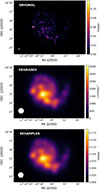 |
Fig. C.3. GALEX FUV map of M 99. Top panel: original map in mJy/px, with an angular resolution of 4.3″ and pixel size of ∼3″. Central panel: degraded map to the SPIRE 500 μm angular resolution (i.e. 36″) in surface brightness units (L⊙ Hz−1 pc−2). Bottom panel: re-projected and re-sampled map to the same orientation and pixel size as SPIRE 500 μm (i.e. px ∼12″) in units of mJy px−1. |
C.4. Reprojection and resampling to the same grid
The final step in the homogenisation process reprojects all images to a common reference frame and resamples them to a uniform pixel size using the reproject_inter Python function15. After resampling, images are converted back to units of Jy px−1.
The bottom panel of Fig. C.3 shows the GALEX FUV map of M 99 after convolution, reprojection, and resampling to the SPIRE 500 μm grid.
C.5. Aperture photometry
The HIP pipeline performs aperture photometry on the target galaxy and estimates the integrated flux uncertainty via a Monte Carlo method (Sect. C.7.3).
Due to M 99’s intrinsic asymmetry, most notably its extended western spiral arm, we adopted and modified the elliptical aperture from Clark et al. (2018) based on visual inspection of our multi-wavelength data. The resulting aperture, shown in Fig. C.4, better aligns with the 5σ contours (white solid lines) and excludes low S/N pixels. Restricting the analysis to pixels within this aperture also reduces the computational cost of the spatially resolved SED fitting. For the Planck/HFI4 band, we measured integrated flux within a circular aperture of radius 300″ to account for the large beam and coarse pixel scale, which spread the galaxy flux over a broader area (Appendix A.3).
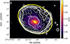 |
Fig. C.4. SPIRE 250 cutout of M 99, overlaid with the ellipse we used for computing the aperture photometry of the galaxy (yellow solid line). For reference, we show the multi-wavelength 5σ contours (white solid lines) of M 99 of all the bands used for SED fitting, listed in Tabs. 2 and 4, at native angular resolution and pixel size. |
HIP additionally computes and plots growth curves (i.e. integrated flux as a function of radius) out to r = 2a, where a is the semi-major axis of the elliptical aperture. Fluxes are summed within co-focal ellipses, serving as diagnostics for sky subtraction quality: the curve should rise within r < a, dominated by galaxy emission, and flatten beyond as noise dominates. Visual inspection confirmed expected growth curve behaviour across bands. Figure C.5 shows the normalised multi-band growth curves, with the adopted aperture indicated in the inset.
 |
Fig. C.5. Multi-band growth curves built by HIP while computing the aperture photometry of M 99. Each measurement (red bars) was computed within larger and larger co-focal ellipses (shown in the inset, overlaid on the SPIRE 250 μm cutout), and then normalised to the corresponding integrated flux (blue dot). The latter was obtained integrating within the yellow ellipse in the inset (see Table 1). Vertical bars show the error (both RMS and flux calibration uncertainty) on the integrated flux. NIKA2 maps are not included here, since the sky subtraction is already performed during the data reduction with Scanam_nika. Planck/HFI4 growth curve is shown in Fig. A.4. |
C.6. CO(2–1) contamination in the millimetre continuum
The CO(2–1) molecular emission line at 230.5 GHz (λ = 1.3 mm) lies within the passbands of both NIKA2 and Planck/HFI4, which have central wavelengths of 1.15 mm and 1.38 mm, respectively, and thus contributes to the measured continuum emission.
The HIP pipeline includes a built-in routine that estimates and subtracts the CO(2–1) line contamination from the millimetre continuum, both on pixel-by-pixel and integrated scales. This routine implements the method described by Drabek et al. (2012). First, it ensures that the CO(2–1) intensity map and the continuum image share the same angular resolution, pixel size, and orientation (performing regridding if necessary). Then, it computes the conversion factor C, which quantifies the fraction of the line flux contributing to the continuum, following Eq. (8) in Drabek et al. (2012):
 (C.1)
(C.1)
where k is Boltzmann’s constant; ν is the line frequency (in GHz); c is the speed of light in km s−1; gν(line) is the filter passband at the frequency of the molecular line; ∫gν dν is the integrated filter passband across the full range of filter frequencies; Ωb is the main beam size.
For M 99, we used the CO(2–1) intensity map from the HERACLES survey (Leroy et al. 2009, Table 3) and computed a contamination factor C = 0.0476 for NIKA2 and C = 50.3 for Planck/HFI4. After subtracting the CO(2–1) contribution, the integrated flux in the NIKA2 1.15 mm map is 0.59 ± 0.04 Jy, with CO(2–1) accounting for ∼9% of the observed flux (0.65 ± 0.04 Jy before correction). For Planck/HFI4, the CO-subtracted flux is 0.35 ± 0.07 Jy, where CO(2–1) contributes about 5% of the total observed 0.37 ± 0.07 Jy.
Figure C.6 shows the spatial distribution of the CO contamination fraction in the NIKA2 1.15 mm continuum (pixels > 3σ), ranging from a few percent up to 20%.
 |
Fig. C.6. Percentage of flux in the NIKA2 1.15 mm map due to CO(2–1) emission line. The beam size (∼13″) is shown at the bottom left. |
C.7. Uncertainty treatment
The HIP pipeline implements a rigorous treatment of uncertainties and ensures their propagation throughout all steps of the pipeline.
C.7.1. Statistical uncertainty
Statistical uncertainty is traditionally estimated from the RMS of flux values measured in regions well separated from the target source. More robust measurements are the 5σ-trimmed standard deviation or the Median Absolute Deviation (MAD), defined as
 (C.2)
(C.2)
where k = 1.4826 for Gaussian distributions. In HIP, the statistical uncertainty is quantified using the MAD computed over the entire image after masking the science source and foreground stars. This approach minimises the impact of random fluctuations from other astrophysical signals or bad pixels.
For images with associated error maps16 (for M 99: Herschel, Spitzer/IRAC 5.2 μm, 8 μm, Spitzer/MIPS 24 μm maps), HIP computes the median of the error map (MeErr) and compares it with the MAD. If MAD > MeErr, MeErr is subtracted in quadrature from the MAD to obtain a flat noise estimate representing residual random fluctuations. This flat noise is then added in quadrature to the original error map pixel-by-pixel, producing the final statistical uncertainty map. Since statistical errors are typically independent or weakly correlated, summing and subtracting in quadrature is justified.
For maps without error maps, the statistical uncertainty is assumed uniform and set equal to the MAD. For NIKA2 maps, the statistical uncertainty is taken as the sky RMS estimated by the Scanam_nika reduction software.
C.7.2. Systematic uncertainty
Notably, HIP accounts for the absolute calibration uncertainty, which represents the bias in the flux measurement introduced by the instrument’s calibration. Table 2 lists the calibration uncertainties for each instrument used in this work. Note that the calibration uncertainty is independent of the noise quantified in Sect. C.7.1.
C.7.3. Uncertainty propagation
Homogenising multi-wavelength images in angular resolution and pixel size reduces statistical uncertainties by averaging over multiple pixels but introduces correlations between adjacent pixels. As a result, standard error propagation methods assuming independent pixels are no longer valid.
To account for this, HIP implements uncertainty propagation via the MC approach. For each image, it draws random noise values per pixel from a normal distribution centred at zero with a standard deviation equal to the pixel’s uncertainty. These noise values are added to the original map, which is then processed through the full homogenisation pipeline. This procedure is repeated over NMC > 100 iterations, generating a cube of perturbed and homogenised maps. The statistical uncertainty map is then computed as the pixel-wise standard deviation across the MC realisations. The total uncertainty map is obtained by adding in quadrature the statistical uncertainty and the calibration uncertainty (Sect. C.7.2).
The same MC approach is used to estimate uncertainties on aperture photometry: the integrated flux is measured on each perturbed map, and the standard deviation across the NMC fluxes provides the statistical uncertainty. Calibration uncertainty is again added in quadrature to derive the total uncertainty.
Appendix D: Validation of our modelling with machine learning predictions
In this Appendix, we validate our modelling by comparing it with the dust maps from Paradis et al. (2024), available in HEALPix format via the CADE website17. These maps were generated using machine learning techniques to predict emission across various Galactic environments and extragalactic sources in the two Planck/HFI bands centred at 850 μm and 1.38 mm. The predicted maps have an angular resolution of approximately 37″, comparable to that of SPIRE 500 μm, and include contributions from synchrotron and free-free emission, which remain below a few percent. Emission from M 99 was predicted based on the KINGFISH survey (Kennicutt et al. 2011) and converted to WCS FITS format using the Drizzweb interface18.
We performed aperture photometry on the predictions from Paradis et al. (2024), obtaining integrated flux densities of S850 = 1.55 ± 0.06 Jy and S1.38 = 0.40 ± 0.03 Jy, after modelling and subtracting the Galactic cirrus contribution. These values agree, within uncertainties, with the fluxes derived from our integrated-scale modelling using HerBIE: S850 = 1.76 ± 0.18 Jy and S1.38 = 0.40 ± 0.04 Jy (THEMIS), and S850 = 1.55 ± 0.16 Jy and S1.38 = 0.31 ± 0.05 Jy (MBB). Our values, however, suggest a slightly steeper millimetre slope.
To enable a direct, spatially resolved comparison, we used our pixel-by-pixel SED decomposition to generate separate dust and radio emission maps of M 99 at 850 μm and 1.38 mm, degraded to the angular resolution of the SPIRE 500 μm data. At a pixel scale of 15″ (∼1.1 kpc), matching that of the Paradis et al. (2024) predictions, the relative differences in flux density between our maps and theirs remain within 10%, in line with typical uncertainties at this resolution. This agreement holds for both the THEMIS and MBB fits.
Appendix E: Pixel masking at low S/N
In Fig. E.1, we highlight in magenta pixels with low S/N, typically located in regions above the 5σ level in the SPIRE 350 μm map but below 3σ in the NIKA2 data (see Figs. 1 and A.1). These pixels often yield unphysical or poorly constrained fitted parameters and were therefore excluded from all quantitative analyses.
 |
Fig. E.1. Magenta regions indicate areas with S/N < 3 in the NIKA2 maps, within the ellipse defining M 99’s geometry (Table 1). These low-S/N regions often show anomalous or extreme model parameter values. Cyan contours show SPIRE 350 μm emission at [5, 15, 35, 55]×σ. The same low-S/N pixels are marked in grey in Figs. 9 (left panel) and 10 for reference. |
Appendix F: Candidate star-forming regions in M 99
In this appendix, we present eight candidate star-forming (SF) regions in M 99, visually selected on the sSFR map as the brightest, isolated, and unresolved sources, consistent with H II regions being smaller than our working resolution of 25″.
Figure F.1 shows the selected SF regions overlaid on the sSFR map. For quantitative analysis, we measured integrated properties within circular apertures of radius 12.5″. The sSFR map was derived by dividing the SFR surface density (Fig. B.2) by the stellar mass surface density (Fig. B.1).
 |
Fig. F.1. Candidate SF regions (green circles) overlaid on the sSFR map of M 99 at 25″ resolution. For reference, cyan contours represent SPIRE 350 μm emission at [5, 15, 35, 55]×σ levels. |
All Tables
Best-fit parameter values obtained with HerBIE (non-hierarchical Bayesian framework) and derived quantities.
Multi-band photometry of the spiral arms, disc, and centre of M 99 computed with HIP.
Best-fit parameter values obtained with HerBIE (non-hierarchical Bayesian framework) for the three morphological components: disc, spiral arms, and galaxy centre.
All Figures
|
Fig. 1. NIKA2 maps of M 99 at 1.15 mm (left) and 2 mm (right) obtained through the Scanam_nika data reduction pipeline in mJy px−1 (cutouts of 8′×6′; pixel size of 3″). The mean RMS is 0.034 mJy px−1 at 1.15 mm and 0.0055 mJy px−1 at 2 mm. White solid lines show the [2.5, 5, 7.5]×σ contours. The FWHM is ∼12″ at 1.15 mm and ∼18″ at 2 mm, corresponding to ∼0.8 and ∼1.25 kpc (see the white circles, bottom-left). |
| In the text | |
|
Fig. 2. Integrated NIR-to-radio SED modelling of M 99 with HerBIE. Filled black circles show observed photometry used in the fit; grey diamonds indicate corresponding synthetic photometry. Left panel: Full SED fit (black line), including stellar emission (starBB, blue), dust emission using powerU with THEMIS (green), and radio continuum (radio, red). Right panel: Fit limited to λ ≥ 100 μm using a single-T MBB (MBB1, green), excluding stellar emission. Empty circles denote data not included in the fit. Residuals are shown below each panel. |
| In the text | |
|
Fig. 3. PHANGS environmental masks by Querejeta et al. (2021) degraded to match SPIRE 250 μm angular resolution (i.e. 18″ ∼ 1.25 kpc) and pixel size (i.e. 6″ ∼ 0.4 kpc). We show the disc in cyan, the spiral arms in blue, and the centre in magenta. For reference, we overlay the IRAC 3.6 μm contours (black solid lines). |
| In the text | |
|
Fig. 4. Near-IR-to-radio SED modelling of the spiral arms (blue), disc (cyan), and centre (magenta) of M 99 with HerBIE. Filled circles show observed photometry; grey diamonds indicate synthetic photometry. Left panel: Full SED fits (solid lines) including stellar emission (starBB, yellow areas); dust emission, using powerU with THEMIS (blue, cyan, magenta areas); and the radio continuum (radio, red areas). Right panel: Fits restricted to λ ≥ 100 μm, modelling dust with single-T MBB (MBB1, coloured areas), and excluding stellar emission. Empty circles were not included in the fit. Monochromatic luminosities (ν Lν) assume a distance of 14.4 Mpc (see Table 1). Residuals are shown below each panel. |
| In the text | |
|
Fig. 5. Pixel-by-pixel χred2 maps at 25″ resolution; bottom-left corner). Left panel: χred2 from the NIR-to-radio SED fitting with THEMIS. Right panel: χred2 from the FIR-to-radio (λ ≥ 100 μm) SED fitting with a single-T MBB. Insets show the χred2 distribution. The dashed black vertical lines indicate a χred2 = 1. Solid cyan lines represent the SPIRE 350 μm contours at [5, 15, 35, 55]×σ. |
| In the text | |
|
Fig. 6. Dust spectral index (β) map derived from spatially resolved SED fitting at 25″ resolution for λ ≥ 100 μm using a single-T MBB model. The inset shows the β distribution; the dashed grey line marks the THEMIS value (β = 1.79). SPIRE 350 μm contours at [5, 15, 35, 55]×σ are overlapped in cyan. |
| In the text | |
|
Fig. 7. Dust spectral index β from the pixel-by-pixel single-T MBB fit versus the molecular gas surface density, |
| In the text | |
|
Fig. 8. Pixel-by-pixel maps at 25″ resolution of: the dust mass surface density, Σdust (top); small grain fraction, qAF (middle); and average interstellar radiation field, ⟨U⟩ (bottom), from the THEMIS fit. SPIRE 350 μm contours at [5, 15, 35, 55]×σ are overlaid in cyan. Insets show the corresponding uncertainty distributions and use the same colour-coding as in the maps. |
| In the text | |
|
Fig. 9. Small grain fraction carrying MIR features (qAF) versus average interstellar radiation field intensity (⟨U⟩). Each filled circle represents a pixel of 8″ ∼ 560 pc, while the angular resolution is 25″ ∼ 1.75 kpc. Pearson correlation coefficients are listed in the top right. Left panel: Pixels colour-coded by total gas surface density ( |
| In the text | |
|
Fig. 10. Synchrotron spectral index (αsync) versus SFR surface density (ΣSFR), colour-coded by total gas surface density ( |
| In the text | |
|
Fig. 11. Dust-to-stellar mass ratio scaling relations with stellar mass surface density (Σ★, top) and gas metallicity (bottom) in M 99. Filled circles show the THEMIS dust masses, colour-coded by molecular gas fraction (fmol); grey hexagons correspond to single-T MBB dust masses. Each symbol represents an 8″ ∼ 560 pc pixel. The angular resolution is 25″ ∼ 1.75 kpc. The bottom panel is restricted to the region covered by the metallicity map (Fig. B.5). Solid red and dashed black lines show the best-fit relations for THEMIS and MBB, respectively; green lines show correlations from Casasola et al. (2022). Red and white diamonds mark integrated values from THEMIS and MBB fits, while filled stars in the top panel indicate disc (cyan), spiral arms (blue), and centre (magenta) averages. Calibration uncertainties are indicated by grey bars near the legend. |
| In the text | |
|
Fig. 12. Dust-to-(total) gas mass ratio scaling relations with stellar mass surface density (Σ★, top) and gas metallicity (bottom) in M 99. Filled circles show THEMIS dust masses, colour-coded by molecular gas fraction (fmol); grey hexagons indicate single-T MBB dust masses. Each point represents an 8″ ∼ 560 pc pixel. The angular resolution is 25″ ∼ 1.75 kpc. The bottom panel covers only regions with metallicity measurements (Fig. B.5). Solid red and dashed black lines show best-fit relations for THEMIS and MBB, respectively; green lines show correlations from Casasola et al. (2022). Red and white diamonds mark integrated values for THEMIS and MBB fits. Calibration uncertainties are indicated by grey bars near the legend. |
| In the text | |
|
Fig. A.1. Scanam_nika filled contours of M 99 (shades of pink; levels of [2.5, 5, 7.5]×σ) at 1.15 mm (top) and at 2 mm (bottom) overlaid with SPIRE 250 μm contours (white solid lines; levels of [5, 15, 35, 55]×σ). |
| In the text | |
|
Fig. A.2. Transfer functions from the SPIRE 250 μm simulations binned as a function of S/N, with 1.15 mm (top panel) and 2 mm (bottom panel) total noise (solid black lines; grey shaded areas show the associated uncertainties), i.e. the sum of high frequency (HF) and low frequency (LF) noise. The noise standard deviation σHF is from a simulation including only high-frequency noise (dashed line). The red curve and red shaded area show the cumulative fraction of the flux that is recovered and the associated uncertainties. |
| In the text | |
|
Fig. A.3. Relative differences between the original and simulated SPIRE 250 μm maps, using 1.15 mm noise and mask (top) and 2 mm noise and mask (bottom). All images are degraded and resampled to the SPIRE 350 μm resolution. The 3σ level from the simulated maps (3σsimu) is shown in black, with corresponding NIKA2 contours in orange. Cyan contours show the original SPIRE 250 μm emission (as in Fig. A.1). Figure insets display the distribution of relative differences (ΔS), with MAD values of 0.06 (1.15 mm) and 0.07 (2 mm), both approximated to 0.1. |
| In the text | |
|
Fig. A.4. Original Planck maps of M 99 at 1.38 mm and 2.1 mm (top panels), overlaid with the circles used for computing the growth curve. The modelled sky maps are shown in the central panels. Bottom panels show the growth curves computed on the original Planck maps (red solid lines) and on the sky-subtracted maps (green solid lines). The blue-filled circles indicate the value of the integrated flux, corresponding to the yellow circles in the top panels (r = 300″). |
| In the text | |
|
Fig. B.1. Stellar mass surface density of M 99. The map is convolved to match NIKA2 angular resolution at 2 mm and pixel size. |
| In the text | |
|
Fig. B.2. Star formation rate density of M 99. The map is shown at 18″ angular resolution and 3″ pixel size, matching NIKA2 at 2 mm. |
| In the text | |
|
Fig. B.3. Atomic gas mass surface density of M 99. Spatial resolution and pixel size are the same as the original HI map, i.e. 30″ and 5″, respectively. |
| In the text | |
|
Fig. B.4. Molecular gas surface density map of M 99. Spatial resolution and pixel size are the same as the original CO(1–0) map, i.e. 25.6″ and 4″, respectively. |
| In the text | |
|
Fig. B.5. Metallicity map of M 99, overlaid with SPIRE 250 μm contours (cyan solid lines; levels of [5, 15, 55, 100]×σ). Spatial resolution and pixel size are the same as the SPIRE 250 μm map. |
| In the text | |
|
Fig. C.1. GALEX NUV map of M 99 (in log scale and at native angular resolution, i.e. 5.3″) where the emission coming from the brightest foreground stars is masked. The position and the geometry of M 99 are highlighted with a white ellipse, defined in Appendix C.5. |
| In the text | |
|
Fig. C.2. Modelled sky emission (3σ threshold) in the SPIRE 250 μm map of M 99 at native angular resolution, i.e. 18″. Cyan crosses mark the centres of the mesh cells. The white ellipse is the same as Fig. C.1. |
| In the text | |
|
Fig. C.3. GALEX FUV map of M 99. Top panel: original map in mJy/px, with an angular resolution of 4.3″ and pixel size of ∼3″. Central panel: degraded map to the SPIRE 500 μm angular resolution (i.e. 36″) in surface brightness units (L⊙ Hz−1 pc−2). Bottom panel: re-projected and re-sampled map to the same orientation and pixel size as SPIRE 500 μm (i.e. px ∼12″) in units of mJy px−1. |
| In the text | |
|
Fig. C.4. SPIRE 250 cutout of M 99, overlaid with the ellipse we used for computing the aperture photometry of the galaxy (yellow solid line). For reference, we show the multi-wavelength 5σ contours (white solid lines) of M 99 of all the bands used for SED fitting, listed in Tabs. 2 and 4, at native angular resolution and pixel size. |
| In the text | |
|
Fig. C.5. Multi-band growth curves built by HIP while computing the aperture photometry of M 99. Each measurement (red bars) was computed within larger and larger co-focal ellipses (shown in the inset, overlaid on the SPIRE 250 μm cutout), and then normalised to the corresponding integrated flux (blue dot). The latter was obtained integrating within the yellow ellipse in the inset (see Table 1). Vertical bars show the error (both RMS and flux calibration uncertainty) on the integrated flux. NIKA2 maps are not included here, since the sky subtraction is already performed during the data reduction with Scanam_nika. Planck/HFI4 growth curve is shown in Fig. A.4. |
| In the text | |
|
Fig. C.6. Percentage of flux in the NIKA2 1.15 mm map due to CO(2–1) emission line. The beam size (∼13″) is shown at the bottom left. |
| In the text | |
|
Fig. E.1. Magenta regions indicate areas with S/N < 3 in the NIKA2 maps, within the ellipse defining M 99’s geometry (Table 1). These low-S/N regions often show anomalous or extreme model parameter values. Cyan contours show SPIRE 350 μm emission at [5, 15, 35, 55]×σ. The same low-S/N pixels are marked in grey in Figs. 9 (left panel) and 10 for reference. |
| In the text | |
|
Fig. F.1. Candidate SF regions (green circles) overlaid on the sSFR map of M 99 at 25″ resolution. For reference, cyan contours represent SPIRE 350 μm emission at [5, 15, 35, 55]×σ levels. |
| In the text | |
Current usage metrics show cumulative count of Article Views (full-text article views including HTML views, PDF and ePub downloads, according to the available data) and Abstracts Views on Vision4Press platform.
Data correspond to usage on the plateform after 2015. The current usage metrics is available 48-96 hours after online publication and is updated daily on week days.
Initial download of the metrics may take a while.