| Issue |
A&A
Volume 709, May 2026
|
|
|---|---|---|
| Article Number | A85 | |
| Number of page(s) | 14 | |
| Section | Cosmology (including clusters of galaxies) | |
| DOI | https://doi.org/10.1051/0004-6361/202453164 | |
| Published online | 05 May 2026 | |
Investigating cosmic strings using large-volume hydrodynamical simulations in the context of JWST’s massive UV-bright galaxies
1
Institute for Theoretical Physics, Goethe University, D-60438 Frankfurt am Main, Germany
2
Department of Physics, Kavli Institute for Astrophysics and Space Research, Massachusetts Institute of Technology, Cambridge, MA 02139, USA
3
Center for Astrophysics | Harvard & Smithsonian, 60 Garden Street, Cambridge, MA 02138, USA
4
Department of Physics, McGill University, Montréal, QC H3A 2T8, Canada
5
Cosmology, Gravity and Astroparticle Physics Group, Center for Theoretical Physics of the Universe, Institute for Basic Science, Daejeon 34126, Korea
6
Department of Physics and Astronomy, York University, 4700 Keele Street, Toronto, ON M3J 1P3, Canada
★ Corresponding authors: This email address is being protected from spambots. You need JavaScript enabled to view it.
; This email address is being protected from spambots. You need JavaScript enabled to view it.
Received:
26
November
2024
Accepted:
16
March
2026
Abstract
Recent observations from the James Webb Space Telescope (JWST) have uncovered an unexpectedly large abundance of massive, UV-bright galaxies at high redshifts, presenting a significant challenge to established galaxy formation models within the standard Lambda cold dark matter (ΛCDM) cosmological framework. Cosmic strings, predicted by a wide range of particle physics theories beyond the standard model, provide a promising potential explanation for these observations. They may act as additional gravitational seeds in the early universe, enhancing the process of high-redshift structure formation, potentially resulting in a more substantial population of massive, efficiently star-forming galaxies. We numerically investigate this prediction in large-volume hydrodynamical simulations using the moving-mesh code AREPO and the well-tested IllustrisTNG galaxy formation model. We evaluate the simulation results in the context of recent JWST data and find that sufficiently energetic cosmic strings produce UV luminosity and stellar mass functions that are in slightly to substantially better agreement with observations at high redshifts. Moreover, we observe that the halos seeded by cosmic strings exhibit a greater efficiency of star formation and enhanced central concentrations. Interestingly, our findings indicate that the simulations incorporating cosmic strings converge with those from a baseline ΛCDM model by redshift z ∼ 6. This convergence suggests that the modified cosmological framework effectively replicates the successful predictions of the standard ΛCDM model at lower redshifts, where observational constraints are significantly stronger. Our results provide compelling evidence that cosmic strings may play a crucial role in explaining the galaxy properties observed by JWST at high redshifts while maintaining consistency with well-established models at later epochs.
Key words: galaxies: evolution / galaxies: formation / galaxies: high-redshift / galaxies: luminosity function / mass function / early Universe
© The Authors 2026
 Open Access article, published by EDP Sciences, under the terms of the Creative Commons Attribution License (https://creativecommons.org/licenses/by/4.0), which permits unrestricted use, distribution, and reproduction in any medium, provided the original work is properly cited.
This article is published in open access under the Subscribe to Open model. This email address is being protected from spambots. You need JavaScript enabled to view it. to support open access publication.
1. Introduction
The launch of the James Webb Space Telescope (JWST; Gardner et al. 2006) has marked the beginning of a new era of precision observations at high redshifts. Recent surveys have revealed a surprisingly large number density of highly UV-luminous (e.g., Harikane et al. 2023a, 2024, 2025; Bouwens et al. 2023; Adams et al. 2024; Donnan et al. 2024; Finkelstein et al. 2024; McLeod et al. 2024; Robertson et al. 2024; though see also Willott et al. 2024), massive (e.g., Weibel et al. 2024; Chworowsky et al. 2024) high-redshift galaxies, significantly exceeding almost all predictions from established galaxy formation models (e.g., Tacchella et al. 2018; Yung et al. 2019; Behroozi et al. 2020; Vogelsberger et al. 2020; Kannan et al. 2022a, 2023). Additionally, some observations have suggested the existence of potentially overmassive galaxies in the early universe (e.g., Labbé et al. 2023; Akins et al. 2023; Xiao et al. 2024; Carniani et al. 2024; Casey et al. 2024).
The majority of these studies rely on photometrically selected galaxy samples, which are subject to uncertainties in spectral energy distribution (SED) fits (e.g., Steinhardt et al. 2023; Endsley et al. 2023) and potentially sensitive to low-redshift interlopers (e.g., Naidu et al. 2022; Fujimoto et al. 2023b; Zavala et al. 2023). However, spectroscopic follow-ups (e.g., Curtis-Lake et al. 2023; Robertson et al. 2023; Wang et al. 2023a; Fujimoto et al. 2023a; Bunker et al. 2023; Bakx et al. 2023; Arrabal Haro et al. 2023; Castellano et al. 2024; D’Eugenio et al. 2024) have generally found good agreement with the photometrically inferred redshifts and UV luminosity functions (UVLFs; e.g., Finkelstein et al. 2024; Harikane et al. 2024, 2025; Naidu et al. 2026).
The compatibility of these observations – or lack thereof – with the standard ΛCDM model of cosmology has been discussed extensively (e.g., Boylan-Kolchin 2023; Biagetti et al. 2023; Ferrara et al. 2023; Finkelstein et al. 2023; Lovell et al. 2023; Mason et al. 2023; Steinhardt et al. 2023; Desprez et al. 2024; Yung et al. 2024) since the first publication of JWST’s early science observations. To date, many compelling potential explanations for these results have been proposed in the literature. Examples within standard ΛCDM cosmology include (i) a top-heavy initial mass function (IMF) at high redshifts (e.g., Inayoshi et al. 2022; Finkelstein et al. 2023; Harikane et al. 2023a; Steinhardt et al. 2023; Yung et al. 2024; Harvey et al. 2025; Lu et al. 2025); (ii) a significantly increased star formation efficiency in high-redshift galaxies (e.g., Dekel et al. 2023; Finkelstein et al. 2024; Ceverino et al. 2024; Chworowsky et al. 2024; Boylan-Kolchin 2025); (iii) field-to-field statistical variance (e.g., Desprez et al. 2024; Willott et al. 2024; iv) increased UV variability due to a bursty star-formation history (SFH; e.g., Shen et al. 2023; Sun et al. 2023a,b; Pallottini & Ferrara 2023; Muñoz et al. 2023; Casey et al. 2024); (v) lack of dust attenuation at high redshifts (e.g., Ferrara et al. 2023; Mason et al. 2023; Finkelstein et al. 2023); and (vi) contributions from active galactic nuclei (AGN; e.g., Inayoshi et al. 2022; Harikane et al. 2023b; Hegde et al. 2024; Chworowsky et al. 2024).
Additionally, a number of proposed modifications to the ΛCDM paradigm have been argued to potentially alleviate this tension (e.g., Liu & Bromm 2022; Menci et al. 2022; Boylan-Kolchin 2023; Jiao et al. 2023; Biagetti et al. 2023; Gong et al. 2023; Hütsi et al. 2023; Shen et al. 2024, 2025; Kumar & Weiner 2025). A notable example is the cosmic string model, with predictions of a large abundance of massive, efficiently star-forming galaxies at z ≳ 10 predating JWST’s first light by several years (e.g., Shlaer et al. 2012)1. Cosmic strings are linear topological defects predicted by a broad range of beyond the standard model (BSM) particle physics theories. Topological defects form in the early universe if the vacuum manifold after a symmetry-breaking phase transition has a nontrivial homotopy group; if this manifold has the topology of a circle, the defects are one-dimensional strings carrying trapped energy.
The simplest model of stable cosmic strings, i.e., the Nambu-Goto model2 (e.g., Vilenkin & Shellard 2000), is fully characterized by only one free parameter: the string tension μ that describes the cosmic strings’ energy per unit length. The string tension is related to the energy scale η of the symmetry breaking phase transition as μ ∼ η2 and typically expressed in terms of the dimensionless3 string tension Gμ, where G is Newton’s constant of gravitation. For detailed reviews on cosmic strings, their proposed formation in specific field theories, as well as their spatial distribution and scaling, see, for example, Brandenberger (1994), Hindmarsh & Kibble (1995), Vilenkin & Shellard (2000), Durrer et al. (2002).
By causality, a network of long cosmic strings and loops will inevitably form in the expanding universe and persist until today in particle physics models admitting cosmic string solutions (Kibble 1980, 1982). Cosmic string loops are generated by the intersections of long strings. A “scaling solution” of the network is rapidly approached after the phase transition, according to which all statistical properties of the network are time-invariant if all distances are scaled to the Hubble radius (Copeland et al. 1992). This is verified by Nambu-Goto simulations (Austin et al. 1993; Albrecht & Turok 1985; Bennett & Bouchet 1988; Allen & Shellard 1990; Vanchurin et al. 2006; Ringeval et al. 2007; Lorenz et al. 2010; Blanco-Pillado et al. 2011, 2014; Auclair et al. 2019; Blanco-Pillado & Olum 2020). However, while the scaling solution of long strings is robust, as it is determined by causality arguments, the scaling distribution of string loops is less certain, being affected by the decay channels of both long strings and loops.
Therefore, the most robust constraints on the string tension come from long-string signals, the strongest one being the upper limit Gμ < 10−7 inferred from cosmic microwave background (CMB) anisotropies (Charnock et al. 2016; Planck Collaboration XXV 2014; Dvorkin et al. 2011). With the assumption that cosmic string loops only lose energy to gravitational radiation, a tighter upper bound Gμ ≲ 10−10 can be inferred from the stochastic gravitational wave background recently detected by millisecond pulsar timing arrays (PTAs; Blanco-Pillado et al. 2021; Afzal et al. 2023; Wang et al. 2023b), but we emphasize that this constraint is less robust due to the uncertainty in the scaling solution of loops. Additionally, we note that the gravitational wave signal is dominated by the smallest loops, while the larger loops contribute most significantly to galaxy formation (e.g., Jiao et al. 2024a). Thus, in this work, we adopt only the robust constraint on the string tension.
Since cosmic string loops are predicted to act as additional gravitational seeds in the early universe – alongside the density fluctuations described by standard ΛCDM cosmology – they provide a well-motivated explanation for enhanced early structure formation and therefore a larger abundance of massive dark matter halos at high redshifts (e.g., Brandenberger 1994; Moessner & Brandenberger 1996; Vilenkin & Shellard 2000). This, in turn, is expected to increase the abundance of massive high-redshift galaxies, such as the ones observed by JWST (Jiao et al. 2023)4.
To investigate this theoretical prediction, as well as the impact of modeling cosmic strings on the high-redshift UVLF, we present results from large-volume (Lbox = 148 cMpc) hydrodynamical simulations using the finite-volume moving-mesh code AREPO (Springel 2010; Pakmor et al. 2016) and the well-tested IllustrisTNG (Springel et al. 2018; Nelson et al. 2018, 2019b; Pillepich et al. 2018; Marinacci et al. 2018; Naiman et al. 2018) galaxy formation model. This further builds on previous work presented in Jiao et al. (2024a) of lower-resolution N-body simulations focusing on high-redshift halo mass functions (HMFs). A crucial advantage of full-physics hydrodynamical simulations in this context is the ability to self-consistently model not only the HMFs, but also the stellar mass functions (SMFs) and UVLFs. Rather than inferring the latter from HMFs of dark matter-only simulations, this directly takes baryonic feedback processes into account, allowing more accurate predictions for direct comparisons to observational data.
This work is organized as follows. We describe our methodology in Sect. 2. The main results, including comparisons to JWST observations and existing ΛCDM simulation predictions, are presented in Sect. 3. Finally, we discuss and summarize our findings in Sect. 4.
2. Methods
An overview of the simulations presented in this work is given in Table 1. In summary, we ran a baseline simulation in standard ΛCDM cosmology, three runs modeling the impact of cosmic string loops with string tension Gμ = 10−8 (CS-8), and three Gμ = 10−10 runs (CS-10) using the same relative distribution of cosmic string loops as the CS-8 runs. All simulations are based on the same ΛCDM initial conditions (ICs), but to improve the statistics of our results, we employ multiple CS-8 and CS-10 runs using different IC modifications described below.
Overview of the simulations.
The ΛCDM ICs were generated at redshift z = 127 using the simulation code GADGET-4 (Springel et al. 2021), a recent update to the GADGET code base (Springel et al. 2001b). They model the initial dark matter distribution using second-order Lagrangian perturbation theory in a periodic, cubic box with side length Lbox = 100 h−1 cMpc = 148 cMpc, resolved by 8503 dark matter particles. The cosmological parameters employed throughout all simulations presented in this work are the following: Ωm = 0.3089, Ωb = 0.0486, ΩΛ = 0.6911, H0 = 100 h km s−1 Mpc−1 = 67.74 km s−1 Mpc−1, σ8 = 0.8159, and ns = 0.9667 (Planck Collaboration XIII 2016).
For the runs including cosmic strings, these ICs are then modified at the initial redshift by computing the changes in dark matter particle positions and velocities due to the gravitational effect of cosmic string loops using the Zel’dovich approximation (Zel’dovich 1970; see also the Appendix of Jiao et al. 2024a). This modification is done separately for each of the runs; the specifics of this step are described in more detail in Sect. 2.1.
For each of the modified ICs, as well as the unmodified ICs generated directly with GADGET-4, we then separately run full-physics hydrodynamical simulations down to redshift z = 6 using the finite-volume moving-mesh code AREPO. The 2 × 8503 dark matter and gas particles in the box volume of (148 cMpc)3 correspond to the dark matter and gas mass resolutions mDM = 1.74 × 10⁸ M⊙ and mgas = 3.24 × 10⁷ M⊙, respectively. The gravitational softening length for both dark matter and star particles is set to 4.4 ckpc. For gas in the simulation volume, the softening is locally adaptive (Springel 2010), i.e., variable depending on cell size, with a minimum softening length of 0.44 ckpc.
We used the IllustrisTNG (e.g., Springel et al. 2018; Nelson et al. 2019b) galaxy formation model, which is an updated version of the Illustris (Vogelsberger et al. 2013, 2014a,b; Torrey et al. 2014) model and has been shown to accurately reproduce a wide range of properties of the observed low-redshift galaxy population (e.g., Nelson et al. 2018, 2021; Springel et al. 2018; Marinacci et al. 2018; Naiman et al. 2018). Particularly relevant for this work is the model’s ability to produce SMFs consistent with observations (Pillepich et al. 2018), as well as realistic star-formation activity (Donnari et al. 2019) at low redshifts. Furthermore, the coupling of this physics model to the radiation hydrodynamics (RHD) extension AREPO-RT (Kannan et al. 2019) in the context of the reionization simulation THESAN (Kannan et al. 2022a,b; Garaldi et al. 2022; Smith et al. 2022; Garaldi et al. 2024) has been shown to make accurate predictions for numerous galaxy population properties at redshifts 5 ≲ z ≲ 10, including UVLFs (Kannan et al. 2022a). However, at very high redshifts – in particular beyond z ≳ 12 – the model, based on concordance ΛCDM cosmology, underpredicts the number density of highly UV-luminous galaxies and their star formation rates (Kannan et al. 2023, in the following K23). In this work, the results of the combined data of several large simulation efforts (K23) based on this model are used as an additional baseline ΛCDM comparison, as well as to determine resolution corrections for the simulations presented in this work (see Sect. 2.2).
The halo and galaxy masses in each of our simulations are determined using the SUBFIND substructure finder (Springel et al. 2001a) based on the friends-of-friends (FOF; Davis et al. 1985) group finder within AREPO. Specifically, the newer variant SUBFIND-HBT based on hierarchical bound-tracing (HBT; Han et al. 2012, 2018) is employed on the fly to extract information about substructure in the simulation volume and its properties at each of the output redshifts z = 6, 7, 8, …, 19.
2.1. Implementation of cosmic string loops in the initial conditions
We modify the simulation’s ICs to include cosmic strings based on the procedures described in Jiao et al. (2024a). The detailed steps used in this work are as follows.
To obtain the masses and positions of cosmic string loops, we sample the loop radii based on the scaling distribution and randomly assign their positions separately in the three runs with string tension Gμ = 10−8, labeled as CS-8-0, CS-8-1, and CS-8-2 (Table 1). The number density of loops per unit radius is given in Appendix A. The mass distribution follows from the radius distribution, as the mass of a loop with radius R is given by Mloop = βμR, where βR describes the mean length of a loop with radius R (see, for example, Brandenberger 1994 for details). We adopt a lower cutoff of 107 M⊙ (105 M⊙) for the loop mass in the CS-8 (CS-10) runs due to the finite computational resources, ensuring that this cutoff is set lower than both the dark matter and gas mass resolution in the simulations.
To allow for a direct comparison, we use these same relative loop distributions for the three CS-10 runs by scaling down the CS-8 masses by a factor of 1/100, while keeping their positions and radii identical. The mass scaling factor is based on the fact that the loop mass is proportional to the string tension. These runs are analogously labeled CS-10-0, CS-10-1, and CS-10-2, where the same final digit x indicates the same relative distributions of loops in the respective CS-8-x and CS-10-x runs. Using the different distributions, we verify that this sampling procedure, based on random number generation in the numerical implementation, does not cause substantial variations in the mass functions of our simulated halo population (Appendix A).
We modify the positions and velocities of dark matter particles according to the gravitational displacement onto cosmic string loops, calculated using the Zel’dovich approximation (for further details, see also Jiao et al. 2024a,b). For this step and the subsequent full-physics runs, the following approximations were made. First, cosmic string loops are treated as point masses, i.e., their radius is considered to be negligible on the scales of interest. This is based on the fact that except for very few (𝒪(1) in each simulation) of the largest loops, the radii of the vast majority of the 9158 cosmic string loops in the simulation box are smaller than the mean separation of dark matter particles. Second, the impact of cosmic string loops is only modeled by the IC modification, i.e., the masses of the loops themselves are neglected during the subsequent evolution of the simulation. We base this approximation on the fact that the total mass of cosmic string loops corresponds to only a very small fraction (𝒪(10−6) for Gμ = 10−8) of the total mass of dark matter; further, the mass of a cosmic string loop does not significantly affect the evolution of a loop-seeded halo after the halo mass exceeds the loop mass (Brandenberger 1994).
2.2. Resolution corrections and baseline ΛCDM data
We apply numerical resolution corrections to the stellar masses and UV magnitudes to mitigate the slightly lower star-formation efficiency caused by the relatively low effective resolution (cf., e.g., Pillepich et al. 2018) of our simulations. For this, we use the data presented in K23, based on the combination of results from the MillenniumTNG (MTNG; Pakmor et al. 2023; Hernández-Aguayo et al. 2023; K23) simulation MTNG740, the THESAN flagship run THESAN-1 (Kannan et al. 2022a), as well as the IllustrisTNG runs TNG50 (Pillepich et al. 2019; Nelson et al. 2019a) and TNG300 (Springel et al. 2018). All of these simulations and ours share the same code base, galaxy formation model, and Planck Collaboration XIII (2016) cosmological parameters, while including both higher-resolution (TNG50, TNG300, THESAN-1) and larger-volume (TNG300, MTNG740) runs, allowing more precise predictions over a larger mass and redshift range than our ΛCDM run alone. For the same reason, the combined data additionally serve as a particularly useful ΛCDM baseline for comparison to our results (Sect. 3).
Specifically, we implement the resolution corrections as outlined in K23, based on the methodology described in Pillepich et al. (2018). This uses the highest-resolution run mentioned above, TNG50, as a baseline, while corrections for successively lower-resolution runs (in order, THESAN, TNG300, MTNG740) are determined by computing the average differences in stellar mass between runs in overlapping halo mass bins (i.e., mass bins well-resolved by both simulations in each of these steps; see K23 for further details). The resolution corrections for UV luminosities are computed analogously to these stellar mass corrections. We add the MTNG740 corrections as constant offsets to the logarithm of the stellar masses and to the UV magnitudes of all galaxies in our simulation. This is based on the fact that our runs have an effective resolution quite similar to the MTNG740 simulation, which has dark matter and gas mass resolutions of mDM = 1.62 × 10⁸ M⊙ and mgas = 3.10 × 10⁷ M⊙, respectively. To ensure self-consistency, allowing us to directly compare results from the simulations with and without cosmic string loops, the same offsets are applied to the ΛCDM run and all CS-8 and CS-10 runs, respectively. Our output redshifts differ slightly from those considered in K23, i.e., zK23 = 8, 9, 10, 11, 12, 15. However, since the resolution corrections are only weakly dependent on redshift5, we use their average values as corrections for our additional output redshifts. Finally, we further investigate the impact of numerical resolution in Appendix B.
3. Results
In this section, we present our results for the HMFs, SMFs, UVLFs, stellar-to-halo mass relation (SHMR), and concentration-mass relation (cMr) from simulations with and without cosmic strings. For the runs with cosmic string loops, we show the combined mass and luminosity functions ϕcombined inferred from all three runs, which are computed as weighted averages given by (Vogelsberger et al. 2020)
 (1)
(1)
where ϕi refers to the mass/luminosity function of the simulation i ∈ {CS-8-0, CS-8-1, CS-8-2} for Gμ = 10−8 or i ∈ {CS-10-0, CS-10-1, CS-10-2} for Gμ = 10−10 (cf. Table 1). Here, Ni is the number of halos (for the HMFs) or galaxies (for the SMFs and UVLFs) in the corresponding mass bin.
3.1. Halo and stellar mass functions
Figure 1 shows the HMFs computed from our baseline ΛCDM run, as well as the runs in which the initial conditions have been modified by the effect of cosmic string loops with string tension Gμ = 10−8 and Gμ = 10−10 at redshifts z = 6, 9, and 12. We additionally plot the Poisson errors of the mass functions and the lowest 95% complete halo mass. The latter refers to the first halo mass bin in which at least 95% of simulated halos have at least one stellar particle; halos with significantly lower masses than this are expected to be poorly resolved by the simulation. We used 20 logarithmically spaced halo mass bins spanning the mass range of 7.5 < log(Mhalo/M⊙) < 12.5.
 |
Fig. 1. Comparison of HMFs from the ΛCDM run (solid black curves) to the runs modeling cosmic strings with string tension Gμ = 10−8 (solid red curves) and Gμ = 10−10 (solid blue curves) with corresponding Poisson errors (shaded error bands) at redshifts z = 6, 9, and 12. Vertical dash-dotted lines indicate the first halo mass bin with 95% completeness (see text for details). We note that these are color-coded analogously to the solid curves, but overlapping in the plots shown here. |
By redshift z = 6, our results from both the CS-8 and the CS-10 runs are converged with the ΛCDM baseline, showing that the impact of the modified cosmology on our HMFs becomes negligible towards lower redshifts. However, as expected from the predictions of analytical mass functions (Jiao et al. 2023), the impact of cosmic string loops with Gμ = 10−8 increases towards higher redshifts. For z ≳ 9, their inclusion results in a significantly higher abundance of halos at the high-mass end, as well as an overall slightly increased amplitude of the HMF. At very early times, as shown in the z = 12 panel, halos in the CS-8 runs both form more abundantly and grow to substantially higher masses than in the other runs. This results in an increased HMF amplitude across all mass ranges, with a particularly pronounced difference at the high-mass end.
However, we find that modeling cosmic strings with string tension Gμ = 10−10 has no significant impact on the HMF based on the resolved population of halos in our runs, instead showing excellent agreement with the ΛCDM run at all output redshifts. We stress, though, that our simulations cannot fully capture all potential effects of Gμ = 10−10 loops: in particular, the most massive loop in the CS-10 runs has a mass of the order mCS, max ∼ 108 M⊙ (see Appendix A), but our simulations do not resolve the internal structure or even the abundance of halos on similar mass scales in a converged way, given our limited dark matter mass resolution. However, since our approach models the gravitational effects of cosmic strings through a modification of the initial conditions – rather than as individual resolved mass particles (Sect. 2.1) – we can still model these as additional gravitational seeds present at very early times (z = 127). We therefore expect a potential impact on halos that eventually grow well beyond the maximum loop mass via the additional gravitational perturbations at early times. This is supported by the substantial impact of the Gμ = 10−8 loops on the HMF at halo masses Mhalo > 1011.5 (Fig. 1), despite the maximum loop mass of mCS, max ∼ 1010 M⊙ in these runs, as well as by the minor differences we observe between the ΛCDM and Gμ = 10−10 runs in Figs. 2 and 3 (discussed further in the following). Nevertheless, there is a significant resolution limitation associated with these runs, as smaller loop-seeded halos themselves are not individually resolved. Based on our available data, we can only place a constraint on the resolved halo and galaxy population (the scales corresponding to JWST high-redshift observations), for which we only see a minimal impact by Gμ = 10−10 loops, while the impact of these loops is likely more substantial for halo masses below our resolution limit. We also note that the structure finder did not identify any bound halos in the simulation volume for the ΛCDM and CS-10 runs at redshifts z ≥ 14 at our resolution, while finding (sub-) halos at all output redshifts for the CS-8 run.
 |
Fig. 2. Simulated SMFs from the ΛCDM run (solid black curves) and the runs modeling cosmic strings with string tension Gμ = 10−8 (solid red curves) and Gμ = 10−10 (solid blue curves) with Poisson errors (shaded error bands) at redshifts z = 6 to z = 14. Vertical dash-dotted lines in the corresponding colors show the median stellar mass of halos within the first 95% complete halo mass bin to provide an indication of the typical minimum stellar mass of numerically well-resolved galaxies (see text). Dashed black curves show the Schechter fit of the simulated SMFs from K23, serving as an additional reference for standard ΛCDM cosmology from higher-resolution and larger-volume simulations using the same galaxy formation model as our runs. We show results from their closest available output redshift zK23 ∼ 15 in the z = 14 panel, indicating the slight redshift discrepancy with a reduced opacity of the dashed curve. Observational JWST data from Weibel et al. (2024), Navarro-Carrera et al. (2024), and Harvey et al. (2025) are shown as gray symbols (at the closest integer redshift, where applicable). Additionally, the dashed green line in the lower right panel indicates the stellar mass of the spectroscopically confirmed massive z ∼ 14 galaxy JADES-GS-z14-0 (Carniani et al. 2024). The predicted number density from our CS-8 runs for such a galaxy at z = 14 exceeds the ΛCDM prediction of K23 at their output redshift zK23 ∼ 15 (zK23 ∼ 12) by roughly 3.5 (1.5) orders of magnitude. |
We show results for the SMFs at redshifts from z = 6 to z = 14 in Fig. 2. The stellar masses are corrected for numerical resolution as described in Sect. 2.2. Additionally, we plot the Schechter function fits (Schechter 1976) of the SMF from K23 as a further ΛCDM reference (cf. Sect. 2.2). This not only provides a more accurate baseline, but is also used as a reference for comparison to our CS-8 results at z = 14, where no halos or galaxies were identified in our CS-10 and ΛCDM runs, as mentioned above.
We additionally indicate the median stellar mass of halos in the first 95% complete halo mass bin (see Fig. 1), i.e., the typical stellar mass of galaxies within the least massive well-resolved halos. As galaxies with lower stellar masses are expected to be increasingly affected by the finite numerical resolution, this gives a rough indication of the typical minimum stellar mass of well-resolved galaxies. However, we note that this resolution limit is a more indirect approximation than that shown for the HMFs due to the scatter in the stellar-to-halo mass relation (since the completeness criterion itself is based on a minimum halo mass, which we associate with an approximately corresponding stellar mass by considering the median stellar mass of such halos).
For comparison with observational JWST data, we also plot the SMF estimates from Weibel et al. (2024), Navarro-Carrera et al. (2024), and Harvey et al. (2025), and indicate the stellar mass of the spectroscopically confirmed, extremely massive z ∼ 14 galaxy JADES-GS-z14-0 (Carniani et al. 2024) in the lower right panel. Where applicable, these values are converted to a Chabrier (2003) IMF based on the factors given in Madau & Dickinson (2014) to be consistent with our simulations. We stress that all shown observational SMF estimates are based on SED fits of photometric JWST NIRCam observations (Rieke et al. 2005) and therefore are still currently subject to significant systematic uncertainty (see Sect. 1).
Notably, the SMF results from our cosmic strings runs are again converging with our ΛCDM results towards lower redshifts, so that all simulated SMFs are largely consistent at z = 6. At higher redshifts, the CS-8 runs predict a significantly larger population of high-mass galaxies than the ΛCDM run and the ΛCDM reference simulations from K23. However, similarly to the HMFs, the SMFs from the CS-10 runs are generally consistent with the ΛCDM results even at higher redshifts, with only a minor difference at the high-mass end at z = 11 and a statistically insignificant difference with respect to Poisson errors at z = 12.
At redshifts z = 6 and z = 8, the observational SMF estimates are broadly consistent with our simulation results, although the Navarro-Carrera et al. (2024) values slightly exceed our predictions at z = 6, which agree more closely with the Weibel et al. (2024) results. Although the Harvey et al. (2025) and Navarro-Carrera et al. (2024) data at z = 8 fit our cosmic strings and ΛCDM SMFs roughly equally well, the Weibel et al. (2024) estimates are somewhat more consistent with our Gμ = 10−8 results at medium-to-high stellar masses, agreeing with them within the cited error bars.
At z = 9, the preference of the Weibel et al. (2024) data points towards the Gμ = 10−8 results becomes even more clear, although we note that these estimates are only upper limits at the high-mass end, as indicated by the gray arrows in the plot. However, the Harvey et al. (2025) data instead match our ΛCDM and Gμ = 10−10 results noticeably better at this redshift, being just barely consistent with the Gμ = 10−8 SMF within their respective uncertainties. Comparing the Harvey et al. (2025) estimates with our results and K23 at z = 11 and z = 12 does not show a conclusive preference for ΛCDM / Gμ = 10−10 or Gμ = 10−8, as the key data points at the high-mass end lie in between the values predicted by the simulations. Only data at lower stellar masses show a preference towards Gμ = 10−8 at z = 11 and toward ΛCDM / Gμ = 10−10 at z = 12. However, we caution that our results are likely to be systematically affected by the finite numerical resolution in this mass range, as indicated in the plots by the dash-dotted lines.
Lastly, we show the comparison of our simulated SMF at z = 14 with the ΛCDM estimate of K23 at the stellar mass of the massive observed galaxy JADES-GS-z14-0, i.e.,  (Carniani et al. 2024). We find that the CS-8 runs predict galaxies with this stellar mass to be approximately 3.5 orders of magnitude more abundant at this high redshift. However, we note that the shown K23 curve is based on results at their closest available output redshift, i.e., zK23 ∼ 15; for reference, the difference between our z = 14 prediction at the same stellar mass and their next-lower available redshift (zK23 ∼ 12) SMF is roughly 1.5 orders of magnitude.
3.2. UV luminosity functions
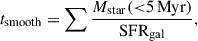
For further comparison with observational data, we show results for our simulated UVLFs in Fig. 3. These are obtained by summing up the radiation output at the rest-frame wavelength 1500 Å in the simulation volume based on tables from BPASS version 2.2.1 (Eldridge et al. 2017). We corrected for numerical artifacts caused by the sparse sampling of the SFH in low-mass halos close to the simulation’s resolution limit by employing the procedure described in Kannan et al. (2022a). Specifically, we smoothed the age and mass of stars formed fewer than 5 Myr ago over the timescale
 (2)
(2)
 |
Fig. 3. Dust-attenuated UV luminosity functions from our baseline ΛCDM run (solid black curves) and modified runs modeling cosmic strings with string tension Gμ = 10−8 (solid red curves) and Gμ = 10−10 (solid blue curves) with corresponding Poisson errors (shaded error bands) at redshifts z = 8 − 16. Dash-dotted vertical lines in the corresponding colors indicate the median UV magnitude of galaxies in the first 95% complete halo mass bin (see Sect. 3.1 for details). At significantly fainter magnitudes than this, the simulation results are expected to be strongly affected by resolution artifacts. Dashed and dotted black curves show Schechter fits of the dust-attenuated UV luminosity functions from higher-resolution and larger-volume ΛCDM simulations using the same code base and galaxy formation model as our runs (K23; Vogelsberger et al. 2020). We note that we show data from the closest available K23 output redshift zK23 for z = 13 (zK23 ∼ 12), as well as for z = 14 and z = 16 (zK23 ∼ 15), and indicate these redshift discrepancies with a reduced opacity of the dashed curve. Green and gray symbols show observational estimates from spectroscopically confirmed (Harikane et al. 2024, 2025; Fujimoto et al. 2024; Napolitano et al. 2025; Naidu et al. 2026) and photometric (Bouwens et al. 2023; Donnan et al. 2023; Harikane et al. 2023a; Pérez-González et al. 2023; Adams et al. 2024; Donnan et al. 2024; Finkelstein et al. 2024; McLeod et al. 2024; Robertson et al. 2024; Willott et al. 2024; Kokorev et al. 2025) JWST data, respectively. Where applicable, these estimates are plotted at the closest integer redshift. At high redshifts z ≳ 11, the observations appear to be in significantly better agreement with the Gμ = 10−8 results than the ΛCDM and Gμ = 10−10 predictions. |
if the corresponding halo satisfies tsmooth > 5 Myr. Here, SFRgal is the instantaneous star-formation rate (SFR) of the host galaxy, computed using the sum of the star formation probabilities of all cells on the equation of state (EoS; Springel & Hernquist 2003). This approach is motivated by the probabilistic star-formation routine used in the physics model, which spawns new star particles stochastically and therefore only occasionally in the lowest-mass halos, and allows a more robust prediction of the UVLF (Kannan et al. 2022a, 2023).
To account for the impact of dust grains, we adopt the empirical dust-attenuation (AUV) model described in K23, which is based on the IRX-UV relation given in Bouwens et al. (2016) from Atacama Large Millimeter Array (ALMA; Wootten & Thompson 2009) observations at z ∼ 4 − 7. Finally, we apply the numerical resolution correction described in Sect. 2.2 to the resulting UV magnitudes MUV.
Figure 3 shows the dust-attenuated UVLFs from our ΛCDM, CS-8, and CS-10 runs at redshifts z = 8 to z = 16. We also include the corresponding Poisson errors, as well as Schechter fits of the dust-attenuated UVLF obtained from the combination of higher-resolution and larger-volume ΛCDM simulations presented in K23. As another reference from higher-resolution runs also using the same simulation code base and galaxy formation model as ours, we additionally plot Vogelsberger et al. (2020) results from post-processing dust radiative transfer calculations using their dust model C at z = 8. Furthermore, we indicate the median UV magnitude of the least massive 95% complete halo mass bin (Sect. 3.1) as a rough estimate of the faintest, but still numerically well-resolved galaxies; however, we stress that this is merely an indirect approximation, since there is typically considerable scatter in the UV magnitudes of galaxies within one halo mass bin. Additionally, since the structure finder did not identify halos in the ΛCDM and CS-10 runs at z ≥ 14, we compare the CS-8 UVLFs with the K23 results at these high redshifts.
Particularly with regard to redshifts z ≳ 12, we also note that the start of star formation tends to be delayed in lower-resolution simulations. Additionally, the latter typically exhibit a suppressed SFR density ρSFR at high redshifts (z ≳ 8) compared to higher-resolution simulations (see e.g. Kannan et al. 2022a, Fig. 12). We attempt to mitigate this effect by our redshift-dependent resolution correction procedure (Sect. 2.2; see also Pillepich et al. 2018; K23), but stress that limited resolution, particularly a delayed onset of star formation, cannot typically be fully corrected for by this prescription (see Appendix B for a more detailed investigation of resolution in our simulations). This is potentially part of the reason for the mismatch between our simulated ΛCDM UVLF and the ΛCDM reference from K23 at z = 13, since it is expected to systematically lower the overall abundance of galaxies in the simulation volume at very high redshifts close to the onset of star formation6. Further, we stress that this redshift, along with z = 14 and z = 16, is not among the K23 output redshifts zK23 for which their UVLF results are available. Therefore, the corresponding plots instead show data from the closest zK23, i.e., zK23 ∼ 12 for the z = 13 panel and zK23 ∼ 15 for the z = 14 and z = 16 panels.
We compare our results with observational UVLF estimates based on both spectroscopically confirmed (Harikane et al. 2025; Fujimoto et al. 2024; Napolitano et al. 2025; Naidu et al. 2026) and photometrically selected (Bouwens et al. 2023; Donnan et al. 2023; Harikane et al. 2023a; Pérez-González et al. 2023; Adams et al. 2024; Donnan et al. 2024; Finkelstein et al. 2024; McLeod et al. 2024; Robertson et al. 2024; Willott et al. 2024; Kokorev et al. 2025) JWST galaxies. Similarly to the HMFs and SMFs, the Gμ = 10−8 UVLFs have a significantly higher amplitude at high redshifts compared to the UVLFs inferred from the other runs. The results show the most marked differences at the UV-bright end, while converging with the ΛCDM and Gμ = 10−10 results towards lower redshifts. Specifically, by redshift z = 8 all of our runs’ UVLFs are in good agreement with each other, as well as with the ΛCDM estimates from K23 and Vogelsberger et al. (2020). Additionally, again there is no significant difference between our Gμ = 10−10 and ΛCDM UVLFs at any of the redshifts considered, except for a mild increase in the predicted abundance of UV-bright galaxies at z = 11.
At redshifts z ≲ 10, all of our predicted UVLFs are generally consistent with observational estimates within the cited error bars, although the Gμ = 10−8 UVLFs begin to show a slight increase at the bright end by z = 10. Notably, as this increase becomes more pronounced at the higher redshifts z = 11 to z = 13, the JWST data show a significant preference toward the Gμ = 10−8 results, again most clearly at the bright end of the UVLFs. At the highest redshifts considered, z = 14 to z = 16, the JWST estimates – including those obtained from observations of spectroscopically confirmed galaxies (Harikane et al. 2024, 2025; Naidu et al. 2026) – clearly show significantly better agreement with the Gμ = 10−8 predictions than the ΛCDM baseline. The remarkable agreement with observational data throughout this broad range of redshifts highlights the Gμ = 10−8 cosmic string model’s potential to produce a galaxy population consistent with both the highest-redshift JWST observations to date and with existing constraints at lower redshifts.
3.3. Stellar-to-halo mass relation and concentration-mass relation
We present results for the SHMR and cMr of halos in our simulations in the following and discuss potential implications in the context of the differences found for the SMFs and UVLFs in previous subsections. Figure 4 shows the SHMR of galaxies from our ΛCDM, CS-8, and CS-10 runs. For each model, we additionally plot the median of the SHMR, computed in 20 logarithmically spaced halo mass bins in the mass range 10.2 < log(Mhalo/M⊙) < 12.5, as well as the 10th to 90th percentile of the distribution. Further, we show the simulated SHMR from K23 as an additional ΛCDM baseline.
 |
Fig. 4. Stellar-to-halo mass ratio of individual simulated galaxies (shaded circles) and median stellar-to-halo mass relation (solid curves) with the 10th to 90th percentile of the distribution (shaded error bands) for our ΛCDM (black), string tension Gμ = 10−8 (red), and Gμ = 10−10 (blue) runs. Shaded circles are only shown for the galaxies outside each mass bin’s shaded error bands to improve readability of the figure. We note that the plots include galaxies from all three separate simulations for each of the string tension values and the single baseline ΛCDM run (cf., Table 1 and Sect. 2). Therefore, the absolute number of Gμ = 10−8 and Gμ = 10−10 scatter points is increased by a factor of three relative to the number of ΛCDM points. We only include halos with masses in or above the first 80% complete halo mass bin (see text for details). Dashed black curves show the stellar-to-halo mass relation from K23 as a further ΛCDM reference. |
In order to remove numerically poorly resolved low-mass halos from our simulations in Fig. 4, we only consider halos with a mass equal to or above the first 80% complete halo mass bin, i.e., the lowest mass bin in which at least 80% of simulated halos have at least one stellar particle and the corresponding galaxies. Within the remaining bins, we then include only the individual halos with at least one stellar particle. For this procedure, we used 20 logarithmically spaced bins over the entire halo mass range, 7.5 < log(Mhalo/M⊙) < 12.5. This is a significantly more stringent resolution criterion than only discarding halos without stellar particles, used to ensure proper convergence of the median SHMR (see also Yeh et al. 2023; K23). However, we note that our 80% completeness cutoff is set to a slightly lower threshold than the 95% completeness indicated in previous sections, or the 100% criterion used in K23, as a reasonable compromise between showing our results in a broader mass range and the stringency of the resolution criterion.
Similarly to previous results, we find no significant differences between the ΛCDM and Gμ = 10−10 median SHMR or its scatter, while the Gμ = 10−8 results show notable differences. Additionally, by redshift z = 8, the median SHMRs of all runs have converged and agree well with the K23 predictions, although we find a slightly increased scatter in the distribution for the CS-8 runs. In particular, there appears to be an increased population of individual massive galaxies within halos of moderate mass in these runs. We find that almost all Gμ = 10−8 galaxies with masses above the 90th percentile (i.e., above the shaded red error band in Fig. 4) correspond to halos seeded by cosmic string loops. However, the relative abundance of these halos is too low to substantially affect the Gμ = 10−8 median SHMR (red curve).
At higher redshifts z ≳ 11, we find a significantly increased median SHMR in the Gμ = 10−8 results across the mass range, with the notable exception of the most massive halos. Although this extremely massive end of the halo mass distribution (Mhalo ≳ 11.4 at z = 11) is only sparsely sampled within our box volume, we note the presence of individual galaxies with very low stellar-to-halo mass fractions in this range. Tracing these galaxies back in time reveals an onset of star formation at typically very high redshifts z ≳ 19, notably followed by a depletion of the galaxies’ gas reservoirs at exceptionally early times and a complete lack of star formation activity thereafter. We plan to further investigate the evolution of these galaxies and their unique star-formation histories in more detail in future work.
Similar individual galaxies are also present at z = 15 in our Gμ = 10−8 results. However, in the mass region of overlap with the K23 data, the Gμ = 10−8 median SHMR is again slightly higher than these predictions based on ΛCDM.
Our results for the SHMR suggest an overall increased efficiency of star formation in halos found in the CS-8 runs at high redshifts compared to ΛCDM or CS-10 halos of similar mass. To investigate a potential reason for this, we turn our attention to the cMr of our simulated halos. We fit the density distribution ρ of our simulated dark matter halos as a function of radius r to the Navarro–Frenk–White density profile (NFW; Navarro et al. 1996)
 (3)
(3)
in log-log space, with the characteristic density ρc and scale radius rs as fit parameters. From this we compute the concentration
 (4)
(4)
where r200 is the radius within which the halo’s mean density is equal to 200 times the critical background density ρcrit. The concentration parameter quantifies the compactness of halos, with a higher concentration indicating a steeper density profile and, in turn, a more compact halo.
In order to estimate the cMr, we sampled 500 of the simulated halos with masses well above the resolution limit, Mhalo ≥ 1010 M⊙, uniformly throughout the simulation volume for the ΛCDM and CS-8-0 runs7, respectively, at each output redshift. Further, we sampled all halos with Mhalo ≥ 1010 M⊙ seeded by the gravitational effects of cosmic string loops in the CS-8-0 run. We identified these loop-seeded halos by their proximity to the coordinates of cosmic string loops in the simulation volume at the first output redshift z = 19 and traced their corresponding FOF group forward in time through our snapshots. We divided the sampled halos into eight logarithmically spaced mass bins in the range 10 < log(Mhalo/M⊙) < 12 and computed the mean and standard deviation of the logarithm of the concentration parameter log c in each bin. The resulting cMr at redshifts z = 6, 9, and 12 is shown in Fig. 5.
 |
Fig. 5. Concentration-mass relation (cMr) of simulated dark matter halos, inferred from a spatially uniform sample of 500 halos in the ΛCDM (black curves) and CS-8-0 (Gμ = 10−8, red curves) runs, as well as from CS-8-0 halos seeded by cosmic string loops (dashed green curves), at redshifts z = 6, 9, and 12. To ensure that individual halos are numerically sufficiently resolved, we only include halos with Mhalo ≥ 1010 M⊙. Filled circles and error bars indicate the mean and standard deviation of the logarithm of the concentrations log c, respectively, in the corresponding mass bins. |
Across the entire redshift range, we find that the mean concentrations of loop-seeded halos are significantly higher than those of ΛCDM halos in all mass bins, indicating that loop-seeded halos tend to be more compact. Additionally, we observe that the concentration of loop-seeded halos tends to increase over time.
In addition, we find that at z ≳ 12, the cMr of the loop-seeded and uniformly sampled CS-8-0 halos is remarkably similar, which indicates that the loop-seeded halos dominate the halo population in the CS-8-0 run at high redshifts. On the other hand, at lower redshifts, the mean concentration of all CS-8-0 halos is considerably lower than that of only loop-seeded halos; by z = 6, the ΛCDM halos clearly dominate the uniform sample. We note that this is consistent with the redshift evolution of both the simulated (Sect. 3.1) and the analytically predicted (Jiao et al. 2023) impact of cosmic string loops on the HMFs.
There are two main factors likely contributing to the higher concentration of loop-seeded halos. Firstly, since they are seeded by point-like sources, loop-seeded halos are expected to have steeper density profiles than those evolved from spatially extended ΛCDM fluctuations (e.g., Mo et al. 2010), which we find to be the case in our simulations. Additionally, since the concentration parameter of a halo tends to increase over time, roughly in proportion to  for a halo initially formed at the time corresponding to the scale factor a = ai (Wechsler et al. 2002), the larger concentrations of loop-seeded halos are indicative of earlier formation times8. This is consistent with the results of our CS-8 simulations, as they are the only runs for which we find resolved halos beyond redshift z = 14, in addition to the HMFs showing a significantly larger population of halos at the high redshifts 9 ≲ z < 14.
In light of these results, an interesting question is whether the higher concentration of loop-seeded halos contributes to their larger median SHMR, as higher concentrations could lead to more rapid gas cooling in their dense inner regions, boosting the initial star formation rate in loop-seeded halos. This may be a potential mechanism producing the highly massive and UV-luminous galaxies found in our simulation volume (Sects. 3.1 and 3.2), or, somewhat more speculatively, the galaxies found by JWST. We plan to investigate the mass assembly histories of loop-seeded halos and the star formation histories of their galaxies in detail in future work.
Additionally, the increased concentration we find for these halos is particularly intriguing given the recent detection of a highly compact, million-solar-mass object at lower redshift (z ∼ 0.881) using gravitational imaging (Powell et al. 2025; Vegetti et al. 2026). Although the simulations presented in this work focus on the high-redshift universe and cannot directly model the substructure at this mass scale given our numerical resolution, we note the qualitative similarity of our results to the fact that this object’s inferred concentration parameter cvir also appears to significantly exceed ΛCDM predictions (Vegetti et al. 2026).
4. Discussion and conclusion
In this work, we have presented a suite of large-volume hydrodynamical simulations to numerically investigate the impact of cosmic string loops with string tensions Gμ = 10−8 and Gμ = 10−10 on the predicted halo and galaxy population at high redshifts. We modify the initial conditions for the simulations, using the Zel’dovich approximation to compute offsets in dark matter particle positions and velocities due to the gravitational effects of cosmic string loops at z = 127. Each of the modified initial conditions then serves as the starting point for a separate full-physics simulation using the AREPO code and IllustrisTNG galaxy formation model. As a ΛCDM baseline, we additionally employ a run based on our unmodified initial conditions, as well as results from previous simulation efforts (K23; Vogelsberger et al. 2020) sharing the same physics model.
We present and compare our results from the simulations with different cosmic string tensions with these ΛCDM predictions; specifically, we show high-redshift (z ≥ 6) predictions for the simulated HMFs and SMFs, UVLFs, SHMR, and cMr. Where applicable, we compare our results with observational estimates from recent JWST data. Our key findings and conclusions are summarized as follows.
-
Modeling cosmic string loops with string tension Gμ = 10−8 results in a substantially larger population of UV-bright galaxies at high redshifts in our simulations. Beyond z ∼ 11, the UV luminosity functions inferred from these runs are in a significantly better agreement with observational JWST estimates than ΛCDM simulation predictions from both this work and the existing literature.
-
Observational SMF estimates appear to slightly favor our Gμ = 10−8 results as well, although we note that this comparison is less conclusive, particularly since estimates from different JWST surveys currently differ significantly. In addition, observational SMF estimates may be subject to uncertainties in the SED modeling and additional assumptions about the high-redshift IMF.
-
Halos in the Gμ = 10−8 simulations show a systematically increased median SHMR at high redshifts z ≳ 11, indicative of more efficient star formation. The latter is frequently invoked as a potentially necessary modification to galaxy formation models in order to achieve consistency with JWST observations (e.g., Dekel et al. 2023; Finkelstein et al. 2024; Ceverino et al. 2024; Chworowsky et al. 2024), typically in the framework of standard ΛCDM cosmology. Our results show the potential of cosmic string models to naturally produce this effect in simulations, without the need to change the physics of the underlying galaxy formation model.
-
We find that halos seeded by Gμ = 10−8 cosmic string loops typically have a higher concentration, determined by a fit to the NFW density profile, than ΛCDM halos of a similar mass. The higher median concentration of loop-seeded halos indicates that they are more compact and therefore likely to have formed at earlier times. We note that this increased compactness may contribute to the higher SHMR we find at high redshifts; we are planning to investigate this possibility in future work.
-
The cosmic string model with string tension Gμ = 10−10 has no significant impact on the properties of the halo or galaxy populations considered in this work; rather, the results of these runs are nearly perfectly consistent with ΛCDM predictions across all redshifts considered. If a string tension of this order or lower were confirmed as a robust upper limit by future observations, our results would therefore tentatively disfavor the cosmic string model as an explanation for JWST observations. However, simulations with higher mass resolution are required to provide more conclusive evidence for or against this explanation (see the discussion on our mass resolution in the context of the Gμ = 10−10 runs in Sect. 3.1).
-
Notably, the results of all our runs converge with the ΛCDM baseline by redshift z = 6 − 8. Therefore, we find good agreement with observational JWST data at the lower redshifts, irrespective of the string tension.
An important limitation of this work is the relatively low resolution of the simulations due to the high computational cost of full-physics hydrodynamical simulations. We tried to mitigate this effect by appropriately rescaling the galaxy properties to higher-resolution simulations performed with the same galaxy formation model and code base (Sect. 2.2). However, numerical resolution affects the timing and efficiency of the earliest star formation in particular, which cannot be fully corrected for with this procedure. Further, since the properties of the string tension Gμ = 10−10 halo and galaxy populations do not differ significantly from the ΛCDM results, our findings are not equipped to provide evidence for or against this particular model.
Future studies are expected to help differentiate the cosmic string model explored in this work from other proposed explanations for the galaxy properties observed by JWST (see Sect. 1). Tighter constraints on the high-redshift SMFs and UVLFs will be made possible by wider-area surveys using, for example, JWST’s NIRCam or Euclid’s wide-field telescope (Euclid Collaboration: Scaramella et al. 2022), as well as by complementary observations at longer wavelengths with, for example, JWST’s Mid-Infrared Instrument (MIRI; Wright et al. 2008) or ALMA; for more detailed discussions, see for example, Weibel et al. (2024), Harikane et al. (2025). We stress that insights from these could substantially alter the interpretation of our results. In particular, our results would provide evidence against the more energetic Gμ = 10−8 cosmic string model if future research established lower values for the SMFs and UVLFs at high redshifts. Crucially, future studies such as precision CMB (Hergt et al. 2017) and 21 cm-line (Brandenberger et al. 2010; Maibach et al. 2021) observations will also be equipped to provide stronger constraints on viable cosmic string tension values.
Acknowledgments
We thank the anonymous referee for constructive feedback and suggestions that helped to improve the paper. We additionally thank Robert Brandenberger, Laura Sagunski, Oliver Zier, and Xuejian (Jacob) Shen for helpful discussions and comments. SMK acknowledges funding from a Goethe University International Lab Visits scholarship and MIT Visiting Student scholarship. HJ is supported in part by an NSERC Discovery Grant to R. Brandenberger, by a Milton Leong Fellowship in Science, and by IBS under the project code IBS-R018-D3. RK acknowledges support of the Natural Sciences and Engineering Research Council of Canada (NSERC) through a Discovery Grant and a Discovery Launch Supplement (funding reference numbers RGPIN-2024-06222 and DGECR-2024-00144) and the support of York University’s Global Research Excellence Initiative. This research was enabled in part by support provided by the Shared Hierarchical Academic Research Computing Network (SHARCNET; www.sharcnet.ca) and Digital Research Alliance of Canada (www.alliancecan.ca). Computations were performed on the Niagara and Trillium supercomputers at the SciNet HPC Consortium (Loken et al. 2010; Ponce et al. 2019). SciNet is funded by Innovation, Science and Economic Development Canada; the Digital Research Alliance of Canada; the Ontario Research Fund: Research Excellence; and the University of Toronto. The higher-resolution runs presented in Appendix B were run on the FASRC Cannon cluster supported by the FAS Division of Science Research Computing Group at Harvard University.
References
- Abbott, R., Abbott, T. D., Abraham, S., et al. 2020, Phys. Rev. Lett., 125, 101102 [Google Scholar]
- Adams, N. J., Conselice, C. J., Austin, D., et al. 2024, ApJ, 965, 169 [NASA ADS] [CrossRef] [Google Scholar]
- Afzal, A., Agazie, G., Anumarlapudi, A., et al. 2023, ApJL, 951, L11 [Google Scholar]
- Akins, H. B., Casey, C. M., Allen, N., et al. 2023, ApJ, 956, 61 [NASA ADS] [CrossRef] [Google Scholar]
- Albrecht, A., & Turok, N. 1985, Phys. Rev. Lett., 54, 1868 [Google Scholar]
- Allen, B., & Shellard, E. P. S. 1990, Phys. Rev. Lett., 64, 119 [Google Scholar]
- Arrabal Haro, P., Dickinson, M., Finkelstein, S. L., et al. 2023, ApJ, 951, L22 [NASA ADS] [CrossRef] [Google Scholar]
- Auclair, P., Ringeval, C., Sakellariadou, M., & Steer, D. 2019, JCAP, 06, 015 [Google Scholar]
- Austin, D., Copeland, E. J., & Kibble, T. W. B. 1993, Phys. Rev. D, 48, 5594 [Google Scholar]
- Bakx, T. J. L. C., Zavala, J. A., Mitsuhashi, I., et al. 2023, MNRAS, 519, 5076 [NASA ADS] [CrossRef] [Google Scholar]
- Behroozi, P., Conroy, C., Wechsler, R. H., et al. 2020, MNRAS, 499, 5702 [NASA ADS] [CrossRef] [Google Scholar]
- Bennett, D. P., & Bouchet, F. R. 1988, Phys. Rev. Lett., 60, 257 [Google Scholar]
- Biagetti, M., Franciolini, G., & Riotto, A. 2023, ApJ, 944, 113 [NASA ADS] [CrossRef] [Google Scholar]
- Blanco-Pillado, J. J., & Olum, K. D. 2020, Phys. Rev. D, 101, 103018 [Google Scholar]
- Blanco-Pillado, J. J., Olum, K. D., & Shlaer, B. 2011, Phys. Rev. D, 83, 083514 [Google Scholar]
- Blanco-Pillado, J. J., Olum, K. D., & Shlaer, B. 2014, Phys. Rev. D, 89, 023512 [NASA ADS] [CrossRef] [Google Scholar]
- Blanco-Pillado, J. J., Olum, K. D., & Wachter, J. M. 2021, Phys. Rev. D, 103, 103512 [NASA ADS] [CrossRef] [Google Scholar]
- Bouwens, R. J., Aravena, M., Decarli, R., et al. 2016, ApJ, 833, 72 [NASA ADS] [CrossRef] [Google Scholar]
- Bouwens, R., Illingworth, G., Oesch, P., et al. 2023, MNRAS, 523, 1009 [NASA ADS] [CrossRef] [Google Scholar]
- Boylan-Kolchin, M. 2023, Nat. Astron., 7, 731 [NASA ADS] [CrossRef] [Google Scholar]
- Boylan-Kolchin, M. 2025, MNRAS, 538, 3210 [Google Scholar]
- Bramberger, S. F., Brandenberger, R. H., Jreidini, P., & Quintin, J. 2015, JCAP, 2015, 007 [Google Scholar]
- Brandenberger, R. H. 1994, Int. J. Mod. Phys. A, 9, 2117 [Google Scholar]
- Brandenberger, R. H., Danos, R. J., Hernández, O. F., & Holder, G. P. 2010, JCAP, 2010, 028 [CrossRef] [Google Scholar]
- Brandenberger, R., Cyr, B., & Jiao, H. 2021, Phys. Rev. D, 104, 123501 [Google Scholar]
- Bunker, A. J., Saxena, A., Cameron, A. J., et al. 2023, A&A, 677, A88 [NASA ADS] [CrossRef] [EDP Sciences] [Google Scholar]
- Carniani, S., Hainline, K., D’Eugenio, F., et al. 2024, Nature, 633, 318 [CrossRef] [Google Scholar]
- Casey, C. M., Akins, H. B., Shuntov, M., et al. 2024, ApJ, 965, 98 [NASA ADS] [CrossRef] [Google Scholar]
- Castellano, M., Napolitano, L., Fontana, A., et al. 2024, ApJ, 972, 143 [Google Scholar]
- Ceverino, D., Nakazato, Y., Yoshida, N., Klessen, R. S., & Glover, S. C. O. 2024, A&A, 689, A244 [NASA ADS] [CrossRef] [EDP Sciences] [Google Scholar]
- Chabrier, G. 2003, PASP, 115, 763 [Google Scholar]
- Charnock, T., Avgoustidis, A., Copeland, E. J., & Moss, A. 2016, Phys. Rev. D, 93, 123503 [Google Scholar]
- Chworowsky, K., Finkelstein, S. L., Boylan-Kolchin, M., et al. 2024, AJ, 168, 113 [NASA ADS] [CrossRef] [Google Scholar]
- Copeland, E. J., Kibble, T. W. B., & Austin, D. 1992, Phys. Rev. D, 45, 1000 [Google Scholar]
- Curtis-Lake, E., Carniani, S., Cameron, A., et al. 2023, Nat. Astron., 7, 622 [NASA ADS] [CrossRef] [Google Scholar]
- Cyr, B., Jiao, H., & Brandenberger, R. 2022, MNRAS, 517, 2221 [Google Scholar]
- Davis, A. C., & Kibble, T. 2005, Contemp. Phys., 46, 313 [Google Scholar]
- Davis, M., Efstathiou, G., Frenk, C. S., & White, S. D. M. 1985, ApJ, 292, 371 [Google Scholar]
- Dekel, A., Sarkar, K. C., Birnboim, Y., Mandelker, N., & Li, Z. 2023, MNRAS, 523, 3201 [NASA ADS] [CrossRef] [Google Scholar]
- Desprez, G., Martis, N. S., Asada, Y., et al. 2024, MNRAS, 530, 2935 [Google Scholar]
- D’Eugenio, F., Maiolino, R., Carniani, S., et al. 2024, A&A, 689, A152 [NASA ADS] [CrossRef] [EDP Sciences] [Google Scholar]
- Donnan, C. T., McLeod, D. J., Dunlop, J. S., et al. 2023, MNRAS, 518, 6011 [Google Scholar]
- Donnan, C. T., McLure, R. J., Dunlop, J. S., et al. 2024, MNRAS, 533, 3222 [NASA ADS] [CrossRef] [Google Scholar]
- Donnari, M., Pillepich, A., Nelson, D., et al. 2019, MNRAS, 485, 4817 [Google Scholar]
- Durrer, R., Kunz, M., & Melchiorri, A. 2002, Phys. Rep., 364, 1 [Google Scholar]
- Dvorkin, C., Wyman, M., & Hu, W. 2011, Phys. Rev. D, 84, 123519 [Google Scholar]
- Eldridge, J. J., Stanway, E. R., Xiao, L., et al. 2017, PASA, 34, e058 [Google Scholar]
- Endsley, R., Stark, D. P., Whitler, L., et al. 2023, MNRAS, 524, 2312 [NASA ADS] [CrossRef] [Google Scholar]
- Euclid Collaboration (Scaramella, R., et al.) 2022, A&A, 662, A112 [NASA ADS] [CrossRef] [EDP Sciences] [Google Scholar]
- Ferrara, A., Pallottini, A., & Dayal, P. 2023, MNRAS, 522, 3986 [NASA ADS] [CrossRef] [Google Scholar]
- Finkelstein, S. L., Bagley, M. B., Ferguson, H. C., et al. 2023, ApJ, 946, L13 [NASA ADS] [CrossRef] [Google Scholar]
- Finkelstein, S. L., Leung, G. C. K., Bagley, M. B., et al. 2024, ApJ, 969, L2 [NASA ADS] [CrossRef] [Google Scholar]
- Fujimoto, S., Arrabal Haro, P., Dickinson, M., et al. 2023a, ApJ, 949, L25 [NASA ADS] [CrossRef] [Google Scholar]
- Fujimoto, S., Finkelstein, S. L., Burgarella, D., et al. 2023b, ApJ, 955, 130 [NASA ADS] [CrossRef] [Google Scholar]
- Fujimoto, S., Wang, B., Weaver, J. R., et al. 2024, ApJ, 977, 250 [NASA ADS] [CrossRef] [Google Scholar]
- Garaldi, E., Kannan, R., Smith, A., et al. 2022, MNRAS, 512, 4909 [NASA ADS] [CrossRef] [Google Scholar]
- Garaldi, E., Kannan, R., Smith, A., et al. 2024, MNRAS, 530, 3765 [Google Scholar]
- Gardner, J. P., Mather, J. C., Clampin, M., et al. 2006, Space Sci. Rev., 123, 485 [Google Scholar]
- Gong, Y., Yue, B., Cao, Y., & Chen, X. 2023, ApJ, 947, 28 [NASA ADS] [CrossRef] [Google Scholar]
- Greene, J. E., Labbe, I., Goulding, A. D., et al. 2024, ApJ, 964, 39 [CrossRef] [Google Scholar]
- Häberle, M., Neumayer, N., Seth, A., et al. 2024, Nature, 631, 285 [CrossRef] [Google Scholar]
- Han, J., Jing, Y. P., Wang, H., & Wang, W. 2012, MNRAS, 427, 2437 [NASA ADS] [CrossRef] [Google Scholar]
- Han, J., Cole, S., Frenk, C. S., Benitez-Llambay, A., & Helly, J. 2018, MNRAS, 474, 604 [CrossRef] [Google Scholar]
- Harikane, Y., Ouchi, M., Oguri, M., et al. 2023a, ApJS, 265, 5 [NASA ADS] [CrossRef] [Google Scholar]
- Harikane, Y., Zhang, Y., Nakajima, K., et al. 2023b, ApJ, 959, 39 [NASA ADS] [CrossRef] [Google Scholar]
- Harikane, Y., Nakajima, K., Ouchi, M., et al. 2024, ApJ, 960, 56 [NASA ADS] [CrossRef] [Google Scholar]
- Harikane, Y., Inoue, A. K., Ellis, R. S., et al. 2025, ApJ, 980, 138 [NASA ADS] [Google Scholar]
- Harvey, T., Conselice, C. J., Adams, N. J., et al. 2025, ApJ, 978, 89 [NASA ADS] [CrossRef] [Google Scholar]
- Hegde, S., Wyatt, M. M., & Furlanetto, S. R. 2024, JCAP, 2024, 025 [CrossRef] [Google Scholar]
- Hergt, L., Amara, A., Brandenberger, R., Kacprzak, T., & Réfrégier, A. 2017, JCAP, 2017, 004 [CrossRef] [Google Scholar]
- Hernández-Aguayo, C., Springel, V., Pakmor, R., et al. 2023, MNRAS, 524, 2556 [CrossRef] [Google Scholar]
- Hindmarsh, M. B., & Kibble, T. W. B. 1995, Rep. Progr. Phys., 58, 477 [Google Scholar]
- Hütsi, G., Raidal, M., Urrutia, J., Vaskonen, V., & Veermäe, H. 2023, Phys. Rev. D, 107, 043502 [CrossRef] [Google Scholar]
- Inayoshi, K., Harikane, Y., Inoue, A. K., Li, W., & Ho, L. C. 2022, ApJ, 938, L10 [NASA ADS] [CrossRef] [Google Scholar]
- Jiao, H., Brandenberger, R., & Refregier, A. 2023, Phys. Rev. D, 108, 043510 [Google Scholar]
- Jiao, H., Brandenberger, R., & Refregier, A. 2024a, Phys. Rev. D, 109, 123524 [Google Scholar]
- Jiao, H., Cyr, B., & Brandenberger, R. 2024b, JCAP, 2024, 069 [Google Scholar]
- Kannan, R., Vogelsberger, M., Marinacci, F., et al. 2019, MNRAS, 485, 117 [CrossRef] [Google Scholar]
- Kannan, R., Garaldi, E., Smith, A., et al. 2022a, MNRAS, 511, 4005 [NASA ADS] [CrossRef] [Google Scholar]
- Kannan, R., Smith, A., Garaldi, E., et al. 2022b, MNRAS, 514, 3857 [CrossRef] [Google Scholar]
- Kannan, R., Springel, V., Hernquist, L., et al. 2023, MNRAS, 524, 2594 [CrossRef] [Google Scholar]
- Kibble, T. W. B. 1976, J. Phys. A Math. Gen., 9, 1387 [Google Scholar]
- Kibble, T. W. B. 1980, Phys. Rep., 67, 183 [Google Scholar]
- Kibble, T. W. B. 1982, Acta Phys. Pol. B, 13, 723 [Google Scholar]
- Kokorev, V., Atek, H., Chisholm, J., et al. 2025, ApJ, 983, L22 [Google Scholar]
- Kumar, S., & Weiner, N. 2025, Phys. Rev. D, 112, 063560 [Google Scholar]
- Labbé, I., van Dokkum, P., Nelson, E., et al. 2023, Nature, 616, 266 [CrossRef] [Google Scholar]
- Liu, B., & Bromm, V. 2022, ApJ, 937, L30 [NASA ADS] [CrossRef] [Google Scholar]
- Loken, C., Gruner, D., Groer, L., et al. 2010, J. Phys. Conf. Ser., 256, 012026 [Google Scholar]
- Lorenz, L., Ringeval, C., & Sakellariadou, M. 2010, JCAP, 10, 003 [CrossRef] [Google Scholar]
- Lovell, C. C., Harrison, I., Harikane, Y., Tacchella, S., & Wilkins, S. M. 2023, MNRAS, 518, 2511 [Google Scholar]
- Lu, S., Frenk, C. S., Bose, S., et al. 2025, MNRAS, 536, 1018 [Google Scholar]
- Madau, P., & Dickinson, M. 2014, ARA&A, 52, 415 [Google Scholar]
- Maibach, D., Brandenberger, R., Crichton, D., & Refregier, A. 2021, Phys. Rev. D, 104, 123535 [Google Scholar]
- Marinacci, F., Vogelsberger, M., Pakmor, R., et al. 2018, MNRAS, 480, 5113 [NASA ADS] [Google Scholar]
- Mason, C. A., Trenti, M., & Treu, T. 2023, MNRAS, 521, 497 [NASA ADS] [CrossRef] [Google Scholar]
- McLeod, D. J., Donnan, C. T., McLure, R. J., et al. 2024, MNRAS, 527, 5004 [Google Scholar]
- Menci, N., Castellano, M., Santini, P., et al. 2022, ApJ, 938, L5 [NASA ADS] [CrossRef] [Google Scholar]
- Mo, H., Van den Bosch, F., & White, S. 2010, Galaxy Formation and Evolution (Cambridge University Press) [Google Scholar]
- Moessner, R., & Brandenberger, R. 1996, MNRAS, 280, 797 [Google Scholar]
- Muñoz, J. B., Mirocha, J., Furlanetto, S., & Sabti, N. 2023, MNRAS, 526, L47 [CrossRef] [Google Scholar]
- Naidu, R. P., Oesch, P. A., Setton, D. J., et al. 2022, arXiv e-prints [arXiv:2208.02794] [Google Scholar]
- Naidu, R. P., Oesch, P. A., Brammer, G., et al. 2026, Open J. Astrophys., 9, 56033 [Google Scholar]
- Naiman, J. P., Pillepich, A., Springel, V., et al. 2018, MNRAS, 477, 1206 [Google Scholar]
- Napolitano, L., Castellano, M., Pentericci, L., et al. 2025, A&A, 693, A50 [NASA ADS] [CrossRef] [EDP Sciences] [Google Scholar]
- Navarro, J. F., Frenk, C. S., & White, S. D. M. 1996, ApJ, 462, 563 [Google Scholar]
- Navarro-Carrera, R., Rinaldi, P., Caputi, K. I., et al. 2024, ApJ, 961, 207 [CrossRef] [Google Scholar]
- Nelson, D., Pillepich, A., Springel, V., et al. 2018, MNRAS, 475, 624 [Google Scholar]
- Nelson, D., Pillepich, A., Springel, V., et al. 2019a, MNRAS, 490, 3234 [Google Scholar]
- Nelson, D., Springel, V., Pillepich, A., et al. 2019b, Comput. Astrophys. Cosmol., 6, 2 [Google Scholar]
- Nelson, E. J., Tacchella, S., Diemer, B., et al. 2021, MNRAS, 508, 219 [NASA ADS] [CrossRef] [Google Scholar]
- Nielsen, H. B., & Olesen, P. 1973, Nucl. Phys. B, 61, 45 [Google Scholar]
- Pacucci, F., & Loeb, A. 2022, MNRAS, 509, 1885 [Google Scholar]
- Pakmor, R., Springel, V., Bauer, A., et al. 2016, MNRAS, 455, 1134 [Google Scholar]
- Pakmor, R., Springel, V., Coles, J. P., et al. 2023, MNRAS, 524, 2539 [NASA ADS] [CrossRef] [Google Scholar]
- Pallottini, A., & Ferrara, A. 2023, A&A, 677, L4 [NASA ADS] [CrossRef] [EDP Sciences] [Google Scholar]
- Pérez-González, P. G., Costantin, L., Langeroodi, D., et al. 2023, ApJ, 951, L1 [CrossRef] [Google Scholar]
- Pillepich, A., Nelson, D., Hernquist, L., et al. 2018, MNRAS, 475, 648 [Google Scholar]
- Pillepich, A., Nelson, D., Springel, V., et al. 2019, MNRAS, 490, 3196 [Google Scholar]
- Planck Collaboration XIII. 2016, A&A, 594, A13 [NASA ADS] [CrossRef] [EDP Sciences] [Google Scholar]
- Planck Collaboration XXV. 2014, A&A, 571, A25 [NASA ADS] [CrossRef] [EDP Sciences] [Google Scholar]
- Ponce, M., van Zon, R., Northrup, S., et al. 2019, in Practice and Experience in Advanced Research Computing 2019: Rise of the Machines (Learning) (New York, NY, USA: Association for Computing Machinery), PEARC ’19 [Google Scholar]
- Powell, D. M., McKean, J. P., Vegetti, S., et al. 2025, Nat. Astron., 9, 1714 [Google Scholar]
- Rees, M. J. 1986, MNRAS, 222, 27P [Google Scholar]
- Rieke, M. J., Kelly, D., & Horner, S. 2005, SPIE Conf. Ser., 5904, 1 [NASA ADS] [Google Scholar]
- Ringeval, C., Sakellariadou, M., & Bouchet, F. 2007, JCAP, 02, 023 [Google Scholar]
- Robertson, B. E., Tacchella, S., Johnson, B. D., et al. 2023, Nat. Astron., 7, 611 [NASA ADS] [CrossRef] [Google Scholar]
- Robertson, B., Johnson, B. D., Tacchella, S., et al. 2024, ApJ, 970, 31 [NASA ADS] [CrossRef] [Google Scholar]
- Schechter, P. 1976, ApJ, 203, 297 [Google Scholar]
- Shen, X., Vogelsberger, M., Boylan-Kolchin, M., Tacchella, S., & Kannan, R. 2023, MNRAS, 525, 3254 [NASA ADS] [CrossRef] [Google Scholar]
- Shen, X., Vogelsberger, M., Boylan-Kolchin, M., Tacchella, S., & Naidu, R. P. 2024, MNRAS, 533, 3923 [Google Scholar]
- Shen, X., Zier, O., Vogelsberger, M., et al. 2025, arXiv e-prints [arXiv:2509.19427] [Google Scholar]
- Shlaer, B., Vilenkin, A., & Loeb, A. 2012, JCAP, 2012, 026 [Google Scholar]
- Silk, J., Begelman, M. C., Norman, C., Nusser, A., & Wyse, R. F. G. 2024, ApJ, 961, L39 [NASA ADS] [CrossRef] [Google Scholar]
- Smith, A., Kannan, R., Garaldi, E., et al. 2022, MNRAS, 512, 3243 [NASA ADS] [CrossRef] [Google Scholar]
- Springel, V. 2010, MNRAS, 401, 791 [Google Scholar]
- Springel, V., & Hernquist, L. 2003, MNRAS, 339, 289 [Google Scholar]
- Springel, V., White, S. D. M., Tormen, G., & Kauffmann, G. 2001a, MNRAS, 328, 726 [Google Scholar]
- Springel, V., Yoshida, N., & White, S. D. M. 2001b, New Astron., 6, 79 [Google Scholar]
- Springel, V., Pakmor, R., Pillepich, A., et al. 2018, MNRAS, 475, 676 [Google Scholar]
- Springel, V., Pakmor, R., Zier, O., & Reinecke, M. 2021, MNRAS, 506, 2871 [NASA ADS] [CrossRef] [Google Scholar]
- Steinhardt, C. L., Kokorev, V., Rusakov, V., Garcia, E., & Sneppen, A. 2023, ApJ, 951, L40 [NASA ADS] [CrossRef] [Google Scholar]
- Sun, G., Faucher-Giguère, C.-A., Hayward, C. C., & Shen, X. 2023a, MNRAS, 526, 2665 [NASA ADS] [CrossRef] [Google Scholar]
- Sun, G., Faucher-Giguère, C.-A., Hayward, C. C., et al. 2023b, ApJ, 955, L35 [CrossRef] [Google Scholar]
- Tacchella, S., Bose, S., Conroy, C., Eisenstein, D. J., & Johnson, B. D. 2018, ApJ, 868, 92 [NASA ADS] [CrossRef] [Google Scholar]
- Torrey, P., Vogelsberger, M., Genel, S., et al. 2014, MNRAS, 438, 1985 [CrossRef] [Google Scholar]
- Turok, N., & Brandenberger, R. H. 1986, Phys. Rev. D, 33, 2175 [Google Scholar]
- Vanchurin, V., Olum, K. D., & Vilenkin, A. 2006, Phys. Rev. D, 74, 063527 [Google Scholar]
- Vegetti, S., White, S. D. M., McKean, J. P., et al. 2026, Nat. Astron., 10, 440 [Google Scholar]
- Vilenkin, A., & Shellard, E. P. S. 2000, Cosmic Strings and Other Topological Defects (Cambridge University Press) [Google Scholar]
- Vogelsberger, M., Genel, S., Sijacki, D., et al. 2013, MNRAS, 436, 3031 [Google Scholar]
- Vogelsberger, M., Genel, S., Springel, V., et al. 2014a, Nature, 509, 177 [Google Scholar]
- Vogelsberger, M., Genel, S., Springel, V., et al. 2014b, MNRAS, 444, 1518 [Google Scholar]
- Vogelsberger, M., Nelson, D., Pillepich, A., et al. 2020, MNRAS, 492, 5167 [NASA ADS] [CrossRef] [Google Scholar]
- Volonteri, M. 2010, A&ARv, 18, 279 [Google Scholar]
- Wang, B., Fujimoto, S., Labbé, I., et al. 2023a, ApJ, 957, L34 [NASA ADS] [CrossRef] [Google Scholar]
- Wang, Z., Lei, L., Jiao, H., Feng, L., & Fan, Y.-Z. 2023b, Sci. China Phys. Mech. Astron., 66, 120403 [Google Scholar]
- Wechsler, R. H., Bullock, J. S., Primack, J. R., Kravtsov, A. V., & Dekel, A. 2002, ApJ, 568, 52 [NASA ADS] [CrossRef] [Google Scholar]
- Weibel, A., Oesch, P. A., Barrufet, L., et al. 2024, MNRAS, 533, 1808 [NASA ADS] [CrossRef] [Google Scholar]
- Willott, C. J., Desprez, G., Asada, Y., et al. 2024, ApJ, 966, 74 [NASA ADS] [CrossRef] [Google Scholar]
- Witten, E. 1985, Phys. Lett. B, 153, 243 [Google Scholar]
- Wootten, A., & Thompson, A. R. 2009, IEEE Proc., 97, 1463 [NASA ADS] [CrossRef] [Google Scholar]
- Wright, G. S., Reike, G., Barella, P., et al. 2008, SPIE Conf. Ser., 7010, 70100T [Google Scholar]
- Wu, X.-B., Wang, F., Fan, X., et al. 2015, Nature, 518, 512 [Google Scholar]
- Xiao, M., Oesch, P. A., Elbaz, D., et al. 2024, Nature, 635, 311 [NASA ADS] [CrossRef] [Google Scholar]
- Yeh, J. Y. C., Smith, A., Kannan, R., et al. 2023, MNRAS, 520, 2757 [NASA ADS] [CrossRef] [Google Scholar]
- Yung, L. Y. A., Somerville, R. S., Finkelstein, S. L., Popping, G., & Davé, R. 2019, MNRAS, 483, 2983 [NASA ADS] [CrossRef] [Google Scholar]
- Yung, L. Y. A., Somerville, R. S., Finkelstein, S. L., Wilkins, S. M., & Gardner, J. P. 2024, MNRAS, 527, 5929 [Google Scholar]
- Zavala, J. A., Buat, V., Casey, C. M., et al. 2023, ApJ, 943, L9 [NASA ADS] [CrossRef] [Google Scholar]
- Zel’dovich, Y. B. 1970, A&A, 5, 84 [NASA ADS] [Google Scholar]
Earlier investigations of cosmic strings recognized their role as potential seeds for structure formation several decades prior, see e.g., Kibble (1976), Rees (1986), Turok & Brandenberger (1986). However, this earlier work focuses on a highly energetic string model now ruled out by cosmic microwave background observations (Planck Collaboration XXV 2014; Charnock et al. 2016).
There are other cosmic string models with more parameters, including string theory models (so-called cosmic superstrings, e.g., Witten 1985; Davis & Kibble 2005), the Abelian Higgs model (Nielsen & Olesen 1973), and superconducting cosmic string models (Witten 1985).
We use natural units in this work, c = kB = ℏ = 1.
We note that a further prediction of these models is the existence of early supermassive black holes (SMBHs; Bramberger et al. 2015; Cyr et al. 2022), another highly-debated source of friction between standard galaxy formation models and high-redshift observations by JWST and previous surveys (see e.g., Volonteri 2010; Wu et al. 2015; Pacucci & Loeb 2022; Silk et al. 2024; Greene et al. 2024), as well as intermediate-mass black holes (IMBHs; Brandenberger et al. 2021), for which strong observational evidence has been found in recent years (Abbott et al. 2020; Häberle et al. 2024).
The redshift-averaged correction value and its standard deviation are (0.40 ± 0.05) dex for the logarithmic stellar masses log(M/M⊙), and ( − 1.32 ± 0.14) mag for the UV magnitudes.
We note that while this may affect the ΛCDM and Gμ = 10−10 results at z = 13, as this is the first redshift for which we find resolved galaxies in these runs, this is not the case for the Gμ = 10−8 simulations due to the much earlier (z > 19) formation of (resolved) galaxies in the latter.
We note that we only sample one of the three CS-8 runs, as it is expected to be representative of all runs with the same string tension; see Appendix A.
We note that this approximate scaling relation is obtained for halos forming and evolving in a ΛCDM cosmology, and does not necessarily generalize to other cosmological models. We therefore explicitly investigated the evolution of loop-seeded halos in our Gμ = 10−8 runs, and similarly found the concentration to grow roughly in proportion to the scale factor.
Appendix A: Distribution of cosmic string loops
The number density n(R, t) dR of cosmic string loops forming at time t in the radius interval between R and R + dR in comoving coordinates is given by (Brandenberger 1994)
 (A.1)
(A.1)
Here, teq is the time of equal matter and radiation, t0 is the present time, and Rcutoff is the loop radius corresponding to our cutoff mass (see Sect. 2.1). Further, N is the mean number of long strings crossing any given Hubble volume, determined by the dynamics of cosmic string networks. The parameters α and β correspond to the ratios between the loop radius and its formation time, and between the loop length and the loop radius, respectively. We assume that the distribution of loops follows the one-scale model, i.e., loops forming at a certain time have the same radius R = αt (α = const.). Typical values of α and β are determined by Nambu-Goto simulations (Austin et al. 1993; Albrecht & Turok 1985; Bennett & Bouchet 1988; Allen & Shellard 1990; Vanchurin et al. 2006; Ringeval et al. 2007; Lorenz et al. 2010; Blanco-Pillado et al. 2011, 2014; Auclair et al. 2019; Blanco-Pillado & Olum 2020). We note that the cutoff radii Rcutoff in our simulations are greater than the minimal loop radius due to gravitational radiation, Rc = ΓGμt, where Γ is the gravitational radiation coefficient (Blanco-Pillado et al. 2021; Wang et al. 2023b). We sample the radii of cosmic string loops from this number density and compute their masses accordingly based on the value of the string tension Gμ (Sect. 2.1). The mass functions of the resulting distributions of cosmic string loops are shown in Fig. A.1.
 |
Fig. A.1. Mass functions of the different distributions of cosmic string loops used in this work. Solid, dashed, and dash-dotted red curves show the mass functions of loops used in our three string tension Gμ = 10−8 (CS-8) simulations. Blue curves show the same for our Gμ = 10−10 (CS-10) runs; the distributions are identical to the Gμ = 10−8 loops, with masses scaled down by a factor of 1/100 (see Sect. 2.1). Poisson errors are shown as shaded error bands in the corresponding colors. |
Additionally, Fig. A.2 shows the halo mass functions computed separately from the different Gμ = 10−8 runs CS-8-0, CS-8-1, and CS-8-2 (see Table 1) at z = 12 as a representative example redshift. Despite minor differences at the very sparsely sampled highest-mass end, the predicted masses of the halo population are all mutually consistent within their respective Poisson uncertainties. We note that we only include the Gμ = 10−8 results in this figure due to the negligible impact of Gμ = 10−10 cosmic string loops on the halo mass function (see Fig. 1). To improve the statistics of our results, we combine the outputs of all three runs with string tension Gμ = 10−8 and Gμ = 10−10, respectively, as described in Sect. 3.
 |
Fig. A.2. Halo mass functions computed separately from the CS-8-0 (solid red curves), CS-8-1 (dashed red curves), and CS-8-2 (dash-dotted red curves) runs (see Table 1). Shaded error bands indicate Poisson errors. |
Appendix B: Convergence tests at higher numerical resolution
To quantify potential numerical resolution effects of our runs remaining after the resolution correction described in Sect. 2.2, we compare results of our original simulations described above with additional, higher-resolution runs using the unmodified (ΛCDM) and string tension Gμ = 10−8 setups. Due to memory constraints on the machine used, we carried out these runs with the same number of particles as the fiducial runs (2 × 8503) at half the box size, Lbox = 50 cMpc h−1 = 74 cMpc. This results in an approximately eight times higher mass resolution, with dark matter and gas mass resolutions of mDM = 2.17 × 10⁷ M⊙ and mgas = 4.05 × 10⁶ M⊙, respectively. Due to the higher effective resolution, we also modified the gravitational softening length for dark matter and star particles to 2.2 ckpc, as well as the minimum softening length for gas to 0.22 ckpc (i.e., half the original values; cf. Sect. 2). Finally, the distribution of the masses and positions of cosmic string loops in the higher-resolution runs with Gμ = 10−8 are identical to a (74 cMpc)3 subset of those of the fiducial CS-8-0 run (Sect. 2.1; App. A).
We run the higher-resolution (HR) simulations down to redshift z = 8, and compare their HMFs (Fig. B.1) and SMFs (Fig. B.2) with those from our original runs at z = 8, 12, and 14 in the following. We apply the same resolution correction procedure as for the main runs (see Sect. 2.2) to the stellar masses, with the corrections recomputed based on these new runs’ resolution, and use the same offsets for both the ΛCDM, HR and Gμ = 10−8, HR runs. Overall, these resolution tests indicate that, in the regime where the resolution and number statistics are sufficiently robust – i.e., excluding the high-mass end where halo numbers are too few in the smaller-box higher-resolution runs, and excluding the low-mass end strongly affected by the lower resolution of the original runs – the higher-resolution simulations are mostly consistent with the runs in the main text.
 |
Fig. B.1. Comparison of halo mass functions inferred from the original runs presented in this paper to those obtained from the higher-resolution (HR) runs performed as a convergence test (see text for details) at redshifts z = 8, 12, and 14. Solid red and black curves indicate the halo mass functions from the original Gμ = 10−8 and ΛCDM runs, respectively. Dashed orange and dark blue curves show halo mass functions from the HR runs using the Gμ = 10−8 and ΛCDM models, respectively. Shaded error bands in the corresponding colors indicate Poisson errors, while vertical-dash dotted lines indicate the first 95% complete halo mass bin (see Sect. 3.1; Fig. 1). |
 |
Fig. B.2. Comparison of stellar mass functions from our original ΛCDM (solid black curves) and Gμ = 10−8 (solid red curves) runs to those inferred from higher-resolution (HR) test runs with Poisson errors (shaded error bands) at redshifts z = 8, 12, and 14. Vertical dash-dotted lines in the corresponding colors indicate the median stellar mass in the first 95% complete halo mass bin (see Sect. 3.1 for details; cf. Fig. 2). |
However, at very high redshifts (z = 12 and 14), we find that this mass range of overlap in which both simulations can produce robust predictions is unfortunately quite small. Due to its smaller simulation volume, the higher-resolution test run can only sparsely sample the rare objects at the high-mass end of the high-redshift halo and galaxy population. Further, the original simulations’ lower resolution causes a characteristic dropoff in the mass functions at the poorly resolved low-mass end, as noted in the main text (see e.g. Fig. 2). We still present comparisons of our runs at these redshifts to fully show the results (and limitations) of our resolution tests – performed within the constraints of the computational resources available for this work – but stress that test runs using a large volume and high resolution would be able to put stronger constraints on our runs’ convergence at very high redshifts.
Fortunately, at a slightly lower redshift (z = 8), a much greater mass range can reliably serve as a direct comparison between simulations. At this redshift, we observe good agreement between the runs for both the HMF and SMF.
Further, in the mass range where both simulations are reliable, the HMFs agree well between the higher- and lower-resolution runs at all redshifts considered. We note, though, that the high-mass end illustrates the poor sampling of the rarest objects in the smaller-volume HR runs at z = 12 and 14, as mentioned above. At z = 12, we find that the SMFs appear to have a slight offset between runs, with the higher-resolution runs predicting an overall slightly lower abundance of galaxies in the intermediate mass range overlapping with predictions from the original runs. However, the prediction of a larger abundance of more massive (Mstellar ≳ 108 M⊙) galaxies in the Gμ = 10−8 HR run compared to the ΛCDM HR run remains robust.
The small overlap of the sufficiently resolved and sampled mass range is unfortunately particularly apparent at z = 14 for the SMFs. We therefore do not attempt to draw overly strong conclusions about the convergence of our simulated stellar masses at such high redshifts, but note that we do find that the overall amplitude and slope appear consistent with the z = 14 SMF obtained from the larger-volume original runs.
All Tables
All Figures
|
Fig. 1. Comparison of HMFs from the ΛCDM run (solid black curves) to the runs modeling cosmic strings with string tension Gμ = 10−8 (solid red curves) and Gμ = 10−10 (solid blue curves) with corresponding Poisson errors (shaded error bands) at redshifts z = 6, 9, and 12. Vertical dash-dotted lines indicate the first halo mass bin with 95% completeness (see text for details). We note that these are color-coded analogously to the solid curves, but overlapping in the plots shown here. |
| In the text | |
|
Fig. 2. Simulated SMFs from the ΛCDM run (solid black curves) and the runs modeling cosmic strings with string tension Gμ = 10−8 (solid red curves) and Gμ = 10−10 (solid blue curves) with Poisson errors (shaded error bands) at redshifts z = 6 to z = 14. Vertical dash-dotted lines in the corresponding colors show the median stellar mass of halos within the first 95% complete halo mass bin to provide an indication of the typical minimum stellar mass of numerically well-resolved galaxies (see text). Dashed black curves show the Schechter fit of the simulated SMFs from K23, serving as an additional reference for standard ΛCDM cosmology from higher-resolution and larger-volume simulations using the same galaxy formation model as our runs. We show results from their closest available output redshift zK23 ∼ 15 in the z = 14 panel, indicating the slight redshift discrepancy with a reduced opacity of the dashed curve. Observational JWST data from Weibel et al. (2024), Navarro-Carrera et al. (2024), and Harvey et al. (2025) are shown as gray symbols (at the closest integer redshift, where applicable). Additionally, the dashed green line in the lower right panel indicates the stellar mass of the spectroscopically confirmed massive z ∼ 14 galaxy JADES-GS-z14-0 (Carniani et al. 2024). The predicted number density from our CS-8 runs for such a galaxy at z = 14 exceeds the ΛCDM prediction of K23 at their output redshift zK23 ∼ 15 (zK23 ∼ 12) by roughly 3.5 (1.5) orders of magnitude. |
| In the text | |
|
Fig. 3. Dust-attenuated UV luminosity functions from our baseline ΛCDM run (solid black curves) and modified runs modeling cosmic strings with string tension Gμ = 10−8 (solid red curves) and Gμ = 10−10 (solid blue curves) with corresponding Poisson errors (shaded error bands) at redshifts z = 8 − 16. Dash-dotted vertical lines in the corresponding colors indicate the median UV magnitude of galaxies in the first 95% complete halo mass bin (see Sect. 3.1 for details). At significantly fainter magnitudes than this, the simulation results are expected to be strongly affected by resolution artifacts. Dashed and dotted black curves show Schechter fits of the dust-attenuated UV luminosity functions from higher-resolution and larger-volume ΛCDM simulations using the same code base and galaxy formation model as our runs (K23; Vogelsberger et al. 2020). We note that we show data from the closest available K23 output redshift zK23 for z = 13 (zK23 ∼ 12), as well as for z = 14 and z = 16 (zK23 ∼ 15), and indicate these redshift discrepancies with a reduced opacity of the dashed curve. Green and gray symbols show observational estimates from spectroscopically confirmed (Harikane et al. 2024, 2025; Fujimoto et al. 2024; Napolitano et al. 2025; Naidu et al. 2026) and photometric (Bouwens et al. 2023; Donnan et al. 2023; Harikane et al. 2023a; Pérez-González et al. 2023; Adams et al. 2024; Donnan et al. 2024; Finkelstein et al. 2024; McLeod et al. 2024; Robertson et al. 2024; Willott et al. 2024; Kokorev et al. 2025) JWST data, respectively. Where applicable, these estimates are plotted at the closest integer redshift. At high redshifts z ≳ 11, the observations appear to be in significantly better agreement with the Gμ = 10−8 results than the ΛCDM and Gμ = 10−10 predictions. |
| In the text | |
|
Fig. 4. Stellar-to-halo mass ratio of individual simulated galaxies (shaded circles) and median stellar-to-halo mass relation (solid curves) with the 10th to 90th percentile of the distribution (shaded error bands) for our ΛCDM (black), string tension Gμ = 10−8 (red), and Gμ = 10−10 (blue) runs. Shaded circles are only shown for the galaxies outside each mass bin’s shaded error bands to improve readability of the figure. We note that the plots include galaxies from all three separate simulations for each of the string tension values and the single baseline ΛCDM run (cf., Table 1 and Sect. 2). Therefore, the absolute number of Gμ = 10−8 and Gμ = 10−10 scatter points is increased by a factor of three relative to the number of ΛCDM points. We only include halos with masses in or above the first 80% complete halo mass bin (see text for details). Dashed black curves show the stellar-to-halo mass relation from K23 as a further ΛCDM reference. |
| In the text | |
|
Fig. 5. Concentration-mass relation (cMr) of simulated dark matter halos, inferred from a spatially uniform sample of 500 halos in the ΛCDM (black curves) and CS-8-0 (Gμ = 10−8, red curves) runs, as well as from CS-8-0 halos seeded by cosmic string loops (dashed green curves), at redshifts z = 6, 9, and 12. To ensure that individual halos are numerically sufficiently resolved, we only include halos with Mhalo ≥ 1010 M⊙. Filled circles and error bars indicate the mean and standard deviation of the logarithm of the concentrations log c, respectively, in the corresponding mass bins. |
| In the text | |
|
Fig. A.1. Mass functions of the different distributions of cosmic string loops used in this work. Solid, dashed, and dash-dotted red curves show the mass functions of loops used in our three string tension Gμ = 10−8 (CS-8) simulations. Blue curves show the same for our Gμ = 10−10 (CS-10) runs; the distributions are identical to the Gμ = 10−8 loops, with masses scaled down by a factor of 1/100 (see Sect. 2.1). Poisson errors are shown as shaded error bands in the corresponding colors. |
| In the text | |
|
Fig. A.2. Halo mass functions computed separately from the CS-8-0 (solid red curves), CS-8-1 (dashed red curves), and CS-8-2 (dash-dotted red curves) runs (see Table 1). Shaded error bands indicate Poisson errors. |
| In the text | |
|
Fig. B.1. Comparison of halo mass functions inferred from the original runs presented in this paper to those obtained from the higher-resolution (HR) runs performed as a convergence test (see text for details) at redshifts z = 8, 12, and 14. Solid red and black curves indicate the halo mass functions from the original Gμ = 10−8 and ΛCDM runs, respectively. Dashed orange and dark blue curves show halo mass functions from the HR runs using the Gμ = 10−8 and ΛCDM models, respectively. Shaded error bands in the corresponding colors indicate Poisson errors, while vertical-dash dotted lines indicate the first 95% complete halo mass bin (see Sect. 3.1; Fig. 1). |
| In the text | |
|
Fig. B.2. Comparison of stellar mass functions from our original ΛCDM (solid black curves) and Gμ = 10−8 (solid red curves) runs to those inferred from higher-resolution (HR) test runs with Poisson errors (shaded error bands) at redshifts z = 8, 12, and 14. Vertical dash-dotted lines in the corresponding colors indicate the median stellar mass in the first 95% complete halo mass bin (see Sect. 3.1 for details; cf. Fig. 2). |
| In the text | |
Current usage metrics show cumulative count of Article Views (full-text article views including HTML views, PDF and ePub downloads, according to the available data) and Abstracts Views on Vision4Press platform.
Data correspond to usage on the plateform after 2015. The current usage metrics is available 48-96 hours after online publication and is updated daily on week days.
Initial download of the metrics may take a while.