| Issue |
A&A
Volume 708, April 2026
|
|
|---|---|---|
| Article Number | L9 | |
| Number of page(s) | 9 | |
| Section | Letters to the Editor | |
| DOI | https://doi.org/10.1051/0004-6361/202659062 | |
| Published online | 03 April 2026 | |
Letter to the Editor
Are supernovae driving turbulence in the solar neighborhood?
1
Université Paris-Saclay, Université Paris Cité, CEA, CNRS, AIM, F-91191 Gif-sur-Yvette, France
2
University of Vienna, Department of Astrophysics, Türkenschanzstraße 17, 1180 Wien, Austria
3
ENS de Lyon, CRAL UMR5574, Universite Claude Bernard Lyon 1, CNRS, Lyon 69007, France
4
Universität Heidelberg, Zentrum für Astronomie, Institut für Theoretische Astrophysik, Albert-Ueberle-Str. 2, 69120 Heidelberg, Germany
5
Universität Heidelberg, Interdisziplinäres Zentrum für Wissenschaftliches Rechnen, Im Neuenheimer Feld 225, 69120 Heidelberg, Germany
6
Laboratoire de Physique de l’Ecole Normale Supérieure, ENS, Université PSL, CNRS, Sorbonne Université, Université Paris Cité, Observatoire de Paris, Paris, France
7
INAF – Istituto di Astrofisica e Planetologia Spaziali, Via Fosso del Cavaliere 100 I-00133, Roma, Italy
8
Dipartimento di Fisica, Università di Roma Tor Vergata, Via della Ricerca Scientifica 1, 00133 Roma, Italy
9
Institute of Physics, Laboratory for Galaxy Evolution and Spectral Modelling, EPFL, Observatoire de Sauverny, Chemin Pegasi 51, 1290 Versoix, Switzerland
★ Corresponding author: This email address is being protected from spambots. You need JavaScript enabled to view it.
Received:
21
January
2026
Accepted:
12
March
2026
Abstract
Context. Turbulence plays an important role in shaping the interstellar medium, and it strongly influences star formation.
Aims. We aim to identify the physical processes capable of sustaining H I turbulence in the solar neighborhood.
Methods. We compare recent H I line-of-sight velocity observations within a volume of radius 70–500 pc centered on the Sun with a suite of 1 kpc numerical simulations that include two distinct turbulent drivers: (i) supernova (SN) feedback and (ii) imposed large-scale turbulent forcing. For each simulation, we constructed synthetic sky maps that closely mimic the observational one, allowing for a consistent comparison between the simulations and the observational data.
Results. The H I observations show a median velocity dispersion of 11.1 km s−1 in the solar neighborhood. The SN-driven simulations systematically underpredict this value, yielding dispersions in the range 4.9–6.7 km s−1. We find that the simulations with strong enough large-scale forcing can reproduce not only the median observed velocity dispersion but also the observed velocity distribution.
Key words: turbulence / ISM: kinematics and dynamics / local insterstellar matter / solar neighborhood
© The Authors 2026
 Open Access article, published by EDP Sciences, under the terms of the Creative Commons Attribution License (https://creativecommons.org/licenses/by/4.0), which permits unrestricted use, distribution, and reproduction in any medium, provided the original work is properly cited.
This article is published in open access under the Subscribe to Open model. This email address is being protected from spambots. You need JavaScript enabled to view it. to support open access publication.
1. Introduction
The interstellar medium (ISM) is the birthplace of stars, and to better understand star formation, it is essential to study the mechanisms that occur in the ISM. Turbulence is one of the main regulators of star formation, alongside gravity (Federrath & Klessen 2012). It plays a dual role, either inducing or opposing gravitational collapse (Mac Low & Klessen 2004).
Many processes contribute to turbulence in the ISM. However, their relative contributions differ, and their importance varies across the different scales (Hennebelle & Falgarone 2012; Klessen & Glover 2016). Several studies (e.g., Wada et al. 2002; Bournaud et al. 2010; Fensch et al. 2023) have shown that large-scale gravitational instabilities, driven by self-gravity and galactic rotation, can sustain ISM turbulence even in the absence of stellar feedback. Other large-scale processes, such as gas accretion into the galaxy, have also been found to be capable of driving turbulence in the ISM (Klessen & Hennebelle 2010). Among the different feedback processes, supernova (SN) explosions from massive stars are believed to dominate the energy injection into the ISM (Klessen & Glover 2016). Each event releases ∼1051 erg in a blast wave, which injects both thermal energy and radial momentum into the surrounding gas. The exact contribution from large driving and SNe remains controversial and may depend on the environment (Iffrig & Hennebelle 2015; Walch et al. 2015; Ohlin et al. 2019).
Krumholz et al. (2018) argue that in galaxies with low gas surface densities, stellar feedback alone can drive turbulence, whereas in gas-rich high-redshift disks, turbulence is mainly sustained by energy injection from large-scale gravitational inflows. A similar result was obtained by Brucy et al. (2020, 2023) using 1 kpc ISM-box simulations. They showed that in gas-rich galaxies, the SN alone cannot sustain enough turbulence to maintain the star formation rate close to observed levels. Observations from Bacchini et al. (2020) showed that in nearby galaxies with low surface density disks, SNe can sustain turbulence without the need for external large-scale drivers. Roman-Oliveira et al. (2024) explored gas-rich galaxies at a redshift of z ≈ 4.5 and found that the measured velocity dispersions were consistent with the feedback-dominated branch of the Krumholz et al. (2018) model. However, they found that including gravitational instabilities overestimated the turbulence.
On smaller scales, simulations of an SN-driven 250-pc-side ISM box by Padoan et al. (2016) showed that SN explosions can drive and sustain turbulence within molecular clouds. By comparing their SN-driven cloud sample with observations from the Outer Galaxy Survey, they obtained consistent cloud statistics and dynamical properties. Colman et al. (2022) compared 1 kpc ISM-box simulations with Herschel observations of the Large Magellanic Cloud and found a similar result on cloud scales. However, on scales larger than ∼60 pc, SN feedback alone is not sufficient, and an additional large-scale driver is required.
We note that H I 21-cm observations have long been used to study the kinematics and turbulence of the neutral ISM in nearby galaxies (McClure-Griffiths et al. 2023). Large surveys such as THINGS (Walter et al. 2008) have provided high-resolution maps of H I across the disks of nearby galaxies. Using these data, Tamburro et al. (2009) found systematically higher velocity dispersions (σH I ≃ 10 ± 2 km s−1) in the inner actively star-forming regions of galaxies and lower dispersions (σH I ≃ 6 km s−1) in the outer H I disks. These results suggest that stellar feedback drives the turbulence in star-forming disks, while large-scale galactic processes maintain a baseline level of turbulence at larger radii.
In the nearby ISM, Soler et al. (2025) (from here on S25) combined three-dimensional dust models from Edenhofer et al. (2024) with H I 21 cm and CO(1−0) emission to construct a spatial map of the line-of-sight (LOS) velocity (vlos) for atomic and molecular gas within a region spanning 70 − 1250 pc in distance and |b|< 5° around the Sun. From these data, they calculated the mean velocity dispersions in H I and CO: σv,H I = 10.8 km s−1 and σv,CO = 6.6 km s−1, respectively.
In this work, we compare the observed dispersions of H I vlos with numerical simulations in which turbulence is driven either by (i) SN feedback or (ii) stochastic Fourier-space forcing, which is meant to represent turbulent energy injected from the large scales. We also include a comparison with the fiducial MHD-4pc run from the TIGRESS suite (Kim & Ostriker 2017), where turbulence is also driven by SN feedback. Our goal is to determine which mechanism can reproduce the observed level of turbulence in the local ISM.
The paper is organized as follows. Section 2 presents a brief description of the numerical simulations used. In Sect. 3, we describe the analysis pipeline and present the velocity dispersion comparison. In Sect. 4, we summarize our findings and evaluate whether SN feedback or large-scale driving can reproduce the observed level of turbulence in the local ISM.
2. Numerical setup
In this section we briefly present the numerical simulations used for comparison with the H I data. The simulations fall into two main families that differ in their mechanism for driving turbulence. Table 1 provides a summary of the main simulation parameters. Section 2.1 introduces the FRIGG simulations, which include both SN-driven and large-scale–forced runs, while Sect. 2.2 presents the SN-driven MHD-4pc simulation from the TIGRESS suite (Kim & Ostriker 2017).
Simulation parameters.
2.1. FRIGG simulations
The FRIGG simulations consist of a suite of three-dimensional simulations of a cubic 1 kpc region of the ISM. The simulations include two distinct families that differ mainly in their turbulence driving mechanism: SN-driven runs (SN), taken from Colman et al. (2025), and large-scale turbulent-forcing runs (TURB), introduced in this work.
These simulations follow a setup similar to that of the FRIGG simulation presented by Hennebelle (2018) and were performed using the adaptive mesh refinement code RAMSES (Teyssier 2002), which solves the equations of ideal magnetohydrodynamics (MHD; Fromang et al. 2006). The base grid consists of 2563 cells, with periodic boundary conditions in the disk plane (x and y) and open boundaries in the vertical (z) direction.
Each simulation begins with an initial turbulent velocity field generated with random phases and a Kolmogorov power spectrum. Turbulence is then sustained either by SN feedback (SN runs) or by stochastic large-scale forcing applied in Fourier space (TURB runs). Details of the turbulence driving prescriptions are provided in Appendix A.
2.2. TIGRESS simulation
Our reference model is the MHD-4pc run of the TIGRESS suite (Kim & Ostriker 2017). It follows a local shearing box that spans Lx = Ly = 1024 pc in the disk plane and Lz = 4096 pc vertically. The grid is uniform, with a 4 pc cell size. The boundary conditions are shearing-periodic in the x direction, periodic in y, and vacuum in z. The simulation starts with an initial k−2 velocity field for t = 50 Myr and then decay it to zero by t = 100 Myr to prevent an artificial collapse burst. After that, turbulence is driven self-consistently by clustered and runaway SNe together with time-dependent far-ultraviolet heating; no external forcing is applied. The simulation reaches a statistical steady state after ∼ 100 Myr and is evolved for a total of 700 Myr. More information about this simulation can be found in their paper. For our analysis, we used the publicly available snapshots1, which consist of a 10243 pc3 sub-volume centered on the mid-plane and cover the interval t ≃ 200−400 Myr.
3. Results
3.1. The dispersions measured by observation
S25 measured LOS H I velocities in the solar neighborhood by combining three-dimensional dust density models from Edenhofer et al. (2024) with H I line emission. This approach allowed them to reconstruct the local H I velocity field. However, the initial reconstruction includes velocity components that may not be physically associated with the local ISM. Instead, they may arise from chance correlations in the method or from nonlocal high-velocity gas along the LOS.
Motivated by the LOS velocities expected in the solar neighborhood from the Galactic rotation model of Reid et al. (2019), S25 imposed a velocity cut of |vlos| ≤ 25 km s−1 on the input H I spectra to mitigate spurious correlations and exclude nonlocal emission. They then subtracted the Galactic rotation model from the reconstructed velocities. In the following, when referring to observational LOS velocities, we always subtract the Galactic rotation model. After subtracting it, the resulting LOS velocities can exceed the original |vlos| ≤ 25 km s−1 cut applied to the input H I spectra.
We restricted the comparison of the simulations to the distance range 70−500 pc. In this range, the maximum LOS velocity after subtracting the model is ∼ 30 km s−1. We therefore adopted |vlos| ≤ 30 km s−1 as the velocity threshold for comparison with the simulations. This choice is further supported by the fact that up to this threshold, the velocity dispersions measured in the inner and outer Galaxy remain comparable, whereas they increasingly diverge at higher velocity thresholds (see Appendix D).
3.2. Line-of-sight velocity construction
To ensure a consistent resolution across all simulations, we first resampled the simulation outputs onto a regular grid with a resolution of 4 pc before constructing the LOS velocity maps. Following S25, we defined the LOS velocity seen by an observer as the projection of the local gas velocity v =(vx,vy,vz) onto the sight-line vector:
 (1)
(1)
Here, x,y,z are the coordinates of the cell relative to the observer, and  .
.
3.2.1. FRIGG boxes.
To minimize the biases that can arise from the choice of a particular position, we placed the observer successively at a set of uniformly spaced positions in the disk mid-plane. Specifically, the observer coordinates were chosen as (xobs,yobs,0), with xobs and yobs taking values between −400 and 500 pc, sampled at intervals of 100 pc. Because the boxes are strictly periodic in (x,y,0), all cell coordinates are rewrapped relative to each observer.
3.2.2. TIGRESS MHD–4pc.
The shearing box is periodic only in y. We therefore shifted the observer along the y-axis in steps of 50 pc, spanning the range −450 ≤ yobs ≤ 500 pc, and along the vertical direction in steps of 25 pc within −25 ≤ zobs ≤ +25 pc to increase the statistical sample. In contrast, xobs was kept fixed to avoid complications associated with shear-periodic boundary conditions. No periodic wrapping was applied in z. The restriction on latitude b (see below) ensures that all sight lines remain close to the mid-plane and do not cross the vertical vacuum boundaries.
We only kept cells with gas temperatures in the range 100 K < T < 10000 K and distances 70 ≤ r ≤ 500 pc. The dependence on the adopted temperature thresholds is examined in Appendix F. The lower distance limit corresponds to the minimum distance covered by the H I data. After applying these spatial cuts, the remaining cells were binned into 4 pc radial bins to match the resolution of the numerical simulations. Positions were then transformed into Galactic coordinates (ℓ,b), and only those with |b| ≤ 5° were kept. Finally, the sky was divided into 10° × 10° longitude-latitude tiles, and mass-weighted averages of the LOS velocity and density were computed for each radial bin and tile.
The H I map has a finer radial resolution (logarithmic bins of 0.4−2.8 pc) and incomplete sky coverage, unlike the simulations. For a consistent comparison at a similar resolution and sampling, we mapped the H I data onto the same (r,ℓ) grid used for the simulations, with linear radial bins spanning 70−500 pc of ≃ 4 pc and longitude bins of 10°. Within each (r,ℓ) cell, we computed the mean and standard deviation of the LOS velocity, and we recorded cells with no data as “NaN”. We then applied the observational (r,ℓ) sampling pattern to the simulation maps (produced from the different observer positions at different time steps) so that only the regions corresponding to observed cells are kept. To minimize any possible biases caused by the nonuniform longitudinal sampling of the observations, we repeated this procedure after rotating the observational grid by 0°, 90°, 180°, and 270° in ℓ, thus producing four masked realizations for each simulation map. In Appendix B we show the LOS velocity map of H I from S25 together with an example of a full simulation map and the four masked versions obtained after applying the different observational samplings.
3.3. Velocity dispersion comparison
After constructing the synthetic sky maps for the different simulations, a velocity cut of |vlos| ≤ 30 km s−1 was applied for a consistent comparison with observations. We then computed the mass-weighted LOS velocity dispersion for each map. Figure 1 shows the obtained distribution of these values. The dot-dashed vertical line in the figure corresponds to the median observed H I velocity dispersion,  , derived in Appendix E from Monte Carlo sampling of LOS velocities reported by S25 using 1000 realizations of the Reid et al. (2019) Galactic rotation model (see Appendix E).
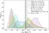 |
Fig. 1. Probability density functions of mass-weighted LOS velocity dispersions for all simulations. Each curve shows the distribution of dispersion values obtained from the different masked sky maps for a given simulation. Dashed curves correspond to the large-scale–forced TURB runs, while dotted curves denote the SN-driven simulations (SN series and TIGRESS-MHD4pc). The dot-dashed vertical line marks the median H I velocity dispersion, |

The SN-driven simulations produced systematically lower velocity dispersions, with mean values of ∼ 4.9−6.7 km s−1, indicating that SN feedback alone underestimates the turbulent level observed in the solar neighborhood. Among the SN-driven simulations, the SN-1.5 and TIGRESS-MHD4pc runs show the largest spreads, with tails reaching and occasionally exceeding the observational value, suggesting that rare SN-driven configurations can attain the required amplitudes but that the typical state remains under-turbulent relative to the data.
As for the large-scale–forced runs, they tend to exhibit higher velocity dispersions at larger forcing amplitudes, with values ranging between ∼9.6 and 15.3 km s−1. The velocity dispersion in TURB-20 exceeds the observational reference, which lies between the values measured for TURB-7 and the intermediate forcing runs TURB-10 and TURB-15. The similar dispersions obtained for these two runs (with TURB-10 slightly higher) despite their different forcing amplitudes are a consequence of the imposed velocity cut, which limits the contribution from the high-velocity tail of the distributions.
Overall, SN-driven turbulence remains systematically weaker than observed. Although SN feedback may dominate turbulence on smaller scales, our results indicate that a large-scale driver is required to reproduce the observed velocity dispersion within the 70−500 pc range considered here.
4. Summary and conclusions
We have compared solar-neighborhood H I LOS velocities from S25 over the distance range of 70−500 pc with two families of 1 kpc box simulations that differ in their turbulence drivers: (i) SN-driven runs, where turbulence is powered solely by SNe, and (ii) large-scale turbulent-forcing runs, where energy is injected at low Fourier modes to mimic the injection from the galactic turbulent cascade. Our comparison of LOS velocity dispersions showed that the SN-driven simulations systematically underpredict the observed H I dispersion. The typical values obtained in the SN runs fall well below the observational range, σobs = 10.8−12 km s−1, inferred from the H I data.
Assuming standard turbulent dissipation, the energy injection rate required to sustain a velocity dispersion, σ, scales as Ė ∝ σ3. This implies that reproducing the observed H I velocity dispersion requires an energy input approximately four to ten times larger than that provided by SN-driven models, and potentially even more if velocities above the adopted 30 km s−1 |vlos| threshold are taken into account. Additional energy injection on large scales is therefore required. In our setup, we find that a large-scale forcing amplitude between those of TURB-7 and intermediate forcing runs (TURB-10 and TURB-15) is sufficient to reproduce the observed velocity dispersion.
We stress that these estimates should be regarded as lower limits since the adopted velocity cut is likely conservative and including higher-velocity gas would further increase the measured dispersion. However, identifying the physical nature of the required large-scale driving will require galactic simulations that include self-consistent galactic-scale physics.
Acknowledgments
This research has received funding from the European Research Council synergy grant ECOGAL (Grant 855130). This work was granted access to HPC resources of CINES and CCRT under the allocation x2020047023 made by GENCI (Grand Equipement National de Calcul Intensif). JDS is funded by the Austrian Science Fund (FWF) through the Principal Investigator Project Grant DOI 10.55776/PAT6169824. NB acknowledges support from the ANR BRIDGES grant (ANR-23-CE31-0005). TC acknowledges funding received from the European High Performance Computing Joint Undertaking (JU) and Belgium, Czech Republic, France, Germany, Greece, Italy, Norway, and Spain under grant agreement no. 101093441 (SPACE).
References
- Bacchini, C., Fraternali, F., Iorio, G., et al. 2020, A&A, 641, A70 [NASA ADS] [CrossRef] [EDP Sciences] [Google Scholar]
- Bate, M. R., Bonnell, I. A., & Price, N. M. 1995, MNRAS, 277, 362 [Google Scholar]
- Bournaud, F., Elmegreen, B. G., Teyssier, R., Block, D. L., & Puerari, I. 2010, MNRAS, 409, 1088 [CrossRef] [Google Scholar]
- Brand, J., & Blitz, L. 1993, A&A, 275, 67 [NASA ADS] [Google Scholar]
- Brucy, N., Hennebelle, P., Bournaud, F., & Colling, C. 2020, ApJ, 896, L34 [NASA ADS] [CrossRef] [Google Scholar]
- Brucy, N., Hennebelle, P., Colman, T., & Iteanu, S. 2023, A&A, 675, A144 [NASA ADS] [CrossRef] [EDP Sciences] [Google Scholar]
- Colman, T., Robitaille, J.-F., Hennebelle, P., et al. 2022, MNRAS, 514, 3670 [NASA ADS] [CrossRef] [Google Scholar]
- Colman, T., Hennebelle, P., Brucy, N., et al. 2025, Open J. Astrophys., 8, 47517 [Google Scholar]
- Edenhofer, G., Zucker, C., Frank, P., et al. 2024, A&A, 685, A82 [NASA ADS] [CrossRef] [EDP Sciences] [Google Scholar]
- Eswaran, V., & Pope, S. B. 1988, Comput. Fluids, 16, 257 [NASA ADS] [CrossRef] [Google Scholar]
- Federrath, C., & Klessen, R. S. 2012, ApJ, 761, 156 [Google Scholar]
- Federrath, C., Banerjee, R., Clark, P. C., & Klessen, R. S. 2010a, ApJ, 713, 269 [NASA ADS] [CrossRef] [Google Scholar]
- Federrath, C., Roman-Duval, J., Klessen, R. S., Schmidt, W., & Mac Low, M.-M. 2010b, A&A, 512, A81 [NASA ADS] [CrossRef] [EDP Sciences] [Google Scholar]
- Fensch, J., Bournaud, F., Brucy, N., et al. 2023, A&A, 672, A193 [NASA ADS] [CrossRef] [EDP Sciences] [Google Scholar]
- Fromang, S., Hennebelle, P., & Teyssier, R. 2006, A&A, 457, 371 [NASA ADS] [CrossRef] [EDP Sciences] [Google Scholar]
- Hennebelle, P. 2018, A&A, 611, A24 [NASA ADS] [CrossRef] [EDP Sciences] [Google Scholar]
- Hennebelle, P., & Falgarone, E. 2012, A&ARv, 20, 55 [NASA ADS] [CrossRef] [Google Scholar]
- Iffrig, O., & Hennebelle, P. 2015, A&A, 576, A95 [CrossRef] [EDP Sciences] [Google Scholar]
- Kim, C.-G., & Ostriker, E. C. 2017, ApJ, 846, 133 [NASA ADS] [CrossRef] [Google Scholar]
- Klessen, R. S., & Glover, S. C. O. 2016, Saas-Fee Advanced Course, 43, 85 [Google Scholar]
- Klessen, R. S., & Hennebelle, P. 2010, A&A, 520, A17 [NASA ADS] [CrossRef] [Google Scholar]
- Krumholz, M. R., Burkhart, B., Forbes, J. C., & Crocker, R. M. 2018, MNRAS, 477, 2716 [CrossRef] [Google Scholar]
- Mac Low, M.-M., & Klessen, R. S. 2004, Rev. Mod. Phys., 76, 125 [Google Scholar]
- McClure-Griffiths, N. M., Stanimirović, S., & Rybarczyk, D. R. 2023, ARA&A, 61, 19 [NASA ADS] [CrossRef] [Google Scholar]
- Ohlin, L., Renaud, F., & Agertz, O. 2019, MNRAS, 485, 3887 [Google Scholar]
- Padoan, P., Pan, L., Haugbølle, T., & Nordlund, Å. 2016, ApJ, 822, 11 [NASA ADS] [CrossRef] [Google Scholar]
- Reid, M. J., Menten, K. M., Brunthaler, A., et al. 2014, ApJ, 783, 130 [Google Scholar]
- Reid, M. J., Menten, K. M., Brunthaler, A., et al. 2019, ApJ, 885, 131 [Google Scholar]
- Roman-Oliveira, F., Rizzo, F., & Fraternali, F. 2024, A&A, 687, A35 [NASA ADS] [CrossRef] [EDP Sciences] [Google Scholar]
- Salpeter, E. E. 1955, ApJ, 121, 161 [Google Scholar]
- Schmidt, W., Niemeyer, J. C., & Hillebrandt, W. 2006, A&A, 450, 265 [NASA ADS] [CrossRef] [EDP Sciences] [Google Scholar]
- Schmidt, W., Federrath, C., Hupp, M., Kern, S., & Niemeyer, J. C. 2009, A&A, 494, 127 [NASA ADS] [CrossRef] [EDP Sciences] [Google Scholar]
- Soler, J. D., Molinari, S., Glover, S. C. O., et al. 2025, A&A, 695, A222 [NASA ADS] [CrossRef] [EDP Sciences] [Google Scholar]
- Tamburro, D., Rix, H.-W., Leroy, A. K., et al. 2009, AJ, 137, 4424 [Google Scholar]
- Teyssier, R. 2002, A&A, 385, 337 [CrossRef] [EDP Sciences] [Google Scholar]
- Tress, R. G., Brucy, N., Girichidis, P., et al. 2025, A&A, submitted [arXiv:2512.09981] [Google Scholar]
- Wada, K., Meurer, G., & Norman, C. A. 2002, ApJ, 577, 197 [NASA ADS] [CrossRef] [Google Scholar]
- Walch, S., Girichidis, P., Naab, T., et al. 2015, MNRAS, 454, 238 [Google Scholar]
- Walter, F., Brinks, E., de Blok, W. J. G., et al. 2008, AJ, 136, 2563 [Google Scholar]
- Wenger, T. V., Balser, D. S., Anderson, L. D., & Bania, T. M. 2018, ApJ, 856, 52 [Google Scholar]
Appendix A: Turbulence driving mechanisms
In this appendix we provide a brief description of the different mechanisms used to drive turbulence in the FRIGG simulations. Section A.1 describes how turbulence is driven by SN feedback in the SN runs, while Sect. A.2 explains how turbulence is driven by large-scale forcing in the TURB runs.
A.1. Supernova driving
In this work, the SN runs adopt a time-dependent UV background, and their numerical suffix indicates the initial mid–plane density (in cm−3). Two members of this series, SN-1 and SN-0.66, were presented in Colman et al. (2025) under the names n1_rms00000 and n0.66_rms00000, respectively.
In these runs sink particles (Bate et al. 1995; Federrath et al. 2010a) are introduced when the density exceeds a threshold of 103 cm−3. These particles can accrete mass from the surrounding gas. Each time sink particles accumulate 120 M⊙, a stellar particle is created with a random mass between 8 and 120 M⊙ drawn from a Salpeter initial mass function (Salpeter 1955). The stellar particle is then assigned a main-sequence lifetime related to its mass. Once this lifetime ends, a SN explosion is triggered, injecting 1051 erg of thermal energy and 4 × 1043 g cm s−1 of radial momentum into the surrounding cells (Iffrig & Hennebelle 2015). To avoid very short time steps, a temperature limit (2 × 10⁶ K) and a velocity limit (200 km s−1) are set.
A.2. Turbulent forcing
In the TURB runs, turbulence is injected following the Ornstein–Uhlenbeck (OU) process (Eswaran & Pope 1988; Schmidt et al. 2006, 2009; Federrath et al. 2010b) as described in Brucy et al. (2023). At each time step (dt ≃ 0.4 Myr), a two–dimensional random acceleration field is evolved in Fourier space, and then transformed back into real space. The forcing is confined to the disk plane and restricted to large-scale Fourier modes with wavelengths between Lbox/3 and Lbox, with the maximum weight assigned to the mode corresponding to a wavelength of Lbox/2. This mimics the injection of kinetic energy from processes at the galactic scale.
We adopt a compressive fraction χ = 0.5 (the ratio of compressive to solenoidal modes contributions), which corresponds to the natural mixture of one-third compressive and two-thirds solenoidal modes projection (Schmidt et al. 2009; Federrath et al. 2010b). The parameter frms controls the power injected by the forcing into the simulation; its value varies in the four runs listed above. Each simulation was evolved for at least two turbulent crossing times, ensuring that the injected turbulence has fully developed throughout the box.
Appendix B: Synthetic and observational sky maps
In this appendix we present a visual comparison between the H I sky map from S25 and an example of the synthetic sky maps generated from the simulations. Figure B.1 shows side–by–side the observational map and a full unmasked synthetic map from the TURB-15 run. Figure B.2 then shows the four masked realizations obtained by applying the observational sampling pattern after rotations of 0°, 90°, 180°, and 270° in longitude. These masked maps are the ones used in the velocity–dispersion analysis.
 |
Fig. B.1. Observed and simulated LOS velocity maps before applying the observational mask. Panel (a): Observed H I LOS velocity map in S25. Panel (b): Example of one full synthetic LOS velocity map from TURB-15. |
 |
Fig. B.2. Masked synthetic sky maps obtained by applying the observational sampling pattern at different rotation angles to the full synthetic map shown in Fig. B.1 (b): Rotation 0° (panel a), 90° (b), 180° (c), and 270° (d). |
Appendix C: Evolution of the velocity PDF
In this appendix we show how the probability density function (PDF) of the line–of–sight velocity evolves purely as a consequence of applying successive numerical processing steps to the simulations.
Figure C.1 shows four panels comparing the H I velocity PDF from S25 (gray histogram; 70–500 pc, |vlos| ≤ 40 km s−1) with the corresponding mass–weighted distribution obtained from one TURB-15 synthetic map (blue), analyzed under four different configurations:
-
Panel a: Point spread function of vlos for all simulation cells satisfying 70 ≤ r ≤ 500 pc and |z|≤rsin5° in the full 4 pc uniform cube (∼6 × 10⁵ cells).
-
Panel b: Same spatial selection, but after collapsing the cube into a 2D (x,y) map by averaging over all cells along the entire vertical LOS (all z at fixed x,y; ∼5 × 10⁴ cells).
-
Panel c: Cells from the synthetic sky projection with 4 pc radial resolution and 10° angular sampling (∼3.8 × 10³ cells).
-
Panel d: Same as panel c, but after applying one of the observational masks (Appendix B), leaving ∼1.2 × 10³ sampled cells.
 |
Fig. C.1. Evolution of the velocity PDF as successive numerical processing steps are applied to one TURB-15 map. The gray histogram shows the H I PDF from S25 (70–500 pc, |vlos| ≤ 40 km s−1). Blue histograms correspond to (A) the intrinsic full-resolution 3D simulation, (B) the 2D (x,y) map obtained by averaging along z, (C) the synthetic sky projection (4 pc radial, 10° angular sampling), and (D) the same projection after applying one observational mask. |
A clear evolution is visible from panels a to d: the intrinsic simulation PDF is smooth, but becomes progressively narrower and more irregular as averaging, angular binning, and sky incompleteness are introduced. This shows that features such as a narrow central peak and long high–velocity tails – characteristic of the observational PDF – can arise from numerical sampling effects alone. We do not claim that every synthetic sky reproduces the observed PDF, but the example shown here illustrates how limited resolution and partial coverage can produce these features.
Appendix D: Dependences on the velocity threshold
In Sect. 3.3, where only velocities up to 30 km s−1 were considered, we showed that SN-driven models yield velocity dispersions below the H I value reported by S25, implying that an additional large-scale driving mechanism is required. The observed values lie between those of the TURB-7 and TURB-10 simulations.
Appendix C further demonstrates that the non-smooth shape of the observed H I LOS velocity PDF, characterized by a sharp central peak and extended high-velocity tails, can be recovered from the simulations once the observational sampling pattern and resolution are applied. This indicates that part of the observed high-velocity structure may arise from resolution and completeness effects and may reflect the way velocities in these ranges are sampled rather than actual physical anomalies.
To estimate how much large-scale forcing would be required if velocities above 30 km s−1 are taken into consideration, we examine how the velocity dispersion varies when imposing different LOS-velocity thresholds, applied to both simulations and observations. Figure D.1 shows the evolution of the average mass-weighted velocity dispersion as a function of the imposed threshold. All simulations display a similar behavior: the dispersion increases with the threshold and eventually saturates once the high-velocity tail is fully recovered. Supernova-driven runs saturate at a threshold of ∼20–25 km s−1, whereas the large-scale-forced runs saturate at significantly higher values, from ∼30–35 km s−1 for TURB-7 up to ∼55 km s−1 for TURB-20.
 |
Fig. D.1. Evolution of the mass-weighted LOS velocity dispersion as a function of the imposed LOS–velocity threshold for both simulations and observations. Colored curves show the simulated models, averaged over the corresponding sets of synthetic sky maps, with SN-driven runs shown as colored dotted lines and large-scale turbulent-forcing runs as colored dashed lines. Black curves correspond to the observational H I data from S25: solid for the full dataset, dotted for the outer Galaxy, and dash-dotted for the inner Galaxy. |
For the observational data, we also separate the inner and outer Galaxy sight lines. Up to ∼35 km s−1, both regions present similar behavior, then they diverge after that, with the inner Galaxy showing larger dispersions. At higher velocity thresholds, the continued increase of the observed velocity dispersion is likely dominated by contamination from noise and contributions from distant, nonlocal high-velocity gas. When comparing simulations with the full Galaxy observational curve, the closest match depends on the chosen threshold: at 30 km s−1TURB-7 matches best; at 40 km s−1 the closest model becomes TURB-10 or TURB-15; and at 50 km s−1, TURB-20 provides the best agreement. However, reliably determining the forcing amplitude required at these higher thresholds will ultimately require more complete sky coverage and more confident H I measurements at high velocities, in order to distinguish genuine turbulent signal from distant motions or instrumental contamination.
Appendix E: Dependences on the Galactic rotation model
In this appendix we consider the effects introduced by the uncertainties in the Galactic rotation models employed to subtract Galactic rotation from kinematic tomography LOS velocity estimates in S25. We focus on the consequences of two aspects of the Galactic rotation model. First, we tested the choice of Galactic rotation model by considering alternatives. Second, we evaluated the effect of uncertainties in the parameters of the Galactic rotation model in Reid et al. (2019).
We considered three alternatives to the Reid et al. (2019) model: a flat rotation curve and the models in Brand & Blitz (1993) and Reid et al. (2014). The Reid et al. (2014) model is the previous iteration of the Reid et al. (2019), obtained with 50% fewer parallax measurements. The Brand & Blitz (1993) model is a landmark reference, based on spectrophotometric distances to H II regions and H I 21-cm emission observations. Finally, the flat rotation curve, constant circular speed with Galactocentric radius, is an acceptable approximation for the Milky Way’s disk dynamics around the solar radius.
Table E.1 presents the standard deviations of the LOS velocities obtained after subtracting the different models of Galactic rotation from the kinematic tomography results in S25. We consider two distance ranges in the input data: 70 < d < 500 pc, which matches the size of the simulation domain, and 70 < d < 1250 pc, which encompasses the distance range in the S25 reconstruction. The results reported in Table E.1 demonstrate that there is very little variation in the resulting standard deviation of noncircular motions, as expected from the nearly constant circular speed around the solar radius. The resulting histograms of residual motions, shown in Fig. E.1, indicate that the global distributions are very similar for the different Galactic rotation models.
 |
Fig. E.1. Same as Fig. 12 in S25 but for three different Galactic rotation models. |
Estimated standard deviation of residual velocities (σv) after subtraction of different Galactic rotation models.
We also tested the effects of the uncertainties in Reid et al. (2019) model parameters. For that purpose, we produce NMC = 1000 realizations of the rotation curve by Monte Carlo sampling its fitted parameters: the Sun distance from the Galactic center (R0), the three-dimensional motion of the Sun in its orbit about the Galaxy (U⊙, V⊙, W⊙), the average peculiar motion of the stars ( ,
,  ), and the universal rotation curve parameters (a2,a3). We sampled the distribution of these parameters using the central values and standard deviations for the A1 model reported in table 3 of (Reid et al. 2019) using the resample_params routine in the kd package (Wenger et al. 2018). Table E.2 presents the resulting mean, median, and standard deviations obtained by subtracting each of the NMC realizations of the circular motions from the kinematic tomography results in S25.
Statistics of standard deviation of residual velocities (σv) for the Monte Carlo sampling of 1000 combinations of the Reid et al. (2019) Galactic rotation models.
Table E.2 presents statistical parameters that characterize the σv distribution for NMC realizations of the Reid et al. (2019) model. Given that σv is a quadratic quantity, it is expected that the mean values are positively biased and the statistical trend is better by the median, which is within 10% of the values reported in S25. The resulting σv standard deviation is also below 10% of the mean and median values of that quantity. Thus, we conclude that the uncertainties in the Reid et al. (2019) model do not significantly challenge the conclusions in S25.
The functional form of the Reid et al. (2019) model implies that σv is unlikely to follow a Gaussian distribution for variations in the input parameters. Thus, we also report the 1st, 25th, 75th, and 99th percentiles of the σv distribution obtained from Monte Carlo sampling. Their values indicate that the distribution is right-skewed, that is, the statistical mode is below the median and the mean. The reported percentiles also indicate that variations in the Reid et al. (2019) model are unlikely to produce significant changes below the median value, 10.5 km/s for H I.
Figure E.2 illustrates the variation in the histograms of residual velocities for a selection of random realizations of the Reid et al. (2019) model. The differences in the histograms show that specific features in the distribution can be introduced by the variations in the subtracted Galactic rotation model. However, the convergence of the mean and median σv values indicates that these excursions are not statistically significant relative to the results of numerical simulations.
 |
Fig. E.2. Same as Fig. 12 in S25 but for the sampling of parameters in the (Reid et al. 2019) Galactic rotation model. |
Appendix F: Dependence on temperature thresholds
In this appendix we investigate how the inferred velocity dispersions depend on the adopted temperature thresholds used to select the H I component in the simulation. Observationally, neutral atomic hydrogen spans a broad temperature range. The cold neutral medium (CNM) typically occupies T ∼ 25–250 K, the unstable neutral medium (UNM) T ∼ 250–4000 K, and the warm neutral medium (WNM) T ∼ 6000–8000 K (McClure-Griffiths et al. 2023). In the FRIGG SN runs, Colman et al. (2025) classify the ISM gas phases using temperature thresholds, with the atomic phases occupying temperatures below ∼ 10000 K. In the TIGRESS simulation (Kim & Ostriker 2017), gas phases are defined using temperature thresholds, with neutral gas below 20000 K and ionized gas above this value. Although molecular hydrogen is present at the lowest temperatures, near those of the CNM, and ionized gas appears at temperatures approaching and exceeding those of the WNM, the total mass over intermediate temperatures is dominated by neutral atomic hydrogen. In their Solar Cirle simulation, Tress et al. (2025) shows that neutral atomic gas dominates the mass distribution particularly between ∼100 and 10000 K where it exceeds both molecular (H2) and ionized (H+) gas. At lower temperatures (≲100 K), the mass is dominated by molecular gas, while at higher temperatures (≳20000, K), the ionized gas becomes the dominant component.
In the main text, we adopt a temperature threshold of 100 < T < 10000 K to approximate the neutral atomic hydrogen component. To assess the robustness of this choice, we recompute the LOS velocity dispersions using three alternative temperature ranges: (1) 0 < T < 10000 K, which includes the coldest neutral atomic gas but also the molecular one; (2) 200 < T < 10000 K, which excludes most of the molecular gas but also removes part of the CNM; (3) 100 < T < 50000 K, to evaluate the impact of including a fraction of the ionized gas.
Figure F.1 shows the distributions of LOS velocity dispersions obtained for different temperature thresholds, for the simulations SN-1.5, TIGRESS-MHD4pc, TURB-7, and TURB-10. Varying the adopted temperature range produces only minor changes in the resulting dispersions. The relative order of the simulations remains unchanged, and the mean values shift by a few tenths of kilometers per second at most. In particular, SN-driven models remain systematically below the observational reference, even when molecular gas is excluded or a fraction of the ionized gas is included, while the large-scale forcing runs continue to exceed it. Our conclusions therefore do not depend sensitively on the adopted temperature range used to approximate the neutral atomic component.
 |
Fig. F.1. Same as Fig. 1 but selecting gas within different temperature ranges: (a) 0 < T < 10000 K; (b) 200 < T < 10000 K; (c) 100 < T < 50000 K. |
All Tables
Estimated standard deviation of residual velocities (σv) after subtraction of different Galactic rotation models.
Statistics of standard deviation of residual velocities (σv) for the Monte Carlo sampling of 1000 combinations of the Reid et al. (2019) Galactic rotation models.
All Figures
|
Fig. 1. Probability density functions of mass-weighted LOS velocity dispersions for all simulations. Each curve shows the distribution of dispersion values obtained from the different masked sky maps for a given simulation. Dashed curves correspond to the large-scale–forced TURB runs, while dotted curves denote the SN-driven simulations (SN series and TIGRESS-MHD4pc). The dot-dashed vertical line marks the median H I velocity dispersion, |
| In the text | |
|
Fig. B.1. Observed and simulated LOS velocity maps before applying the observational mask. Panel (a): Observed H I LOS velocity map in S25. Panel (b): Example of one full synthetic LOS velocity map from TURB-15. |
| In the text | |
|
Fig. B.2. Masked synthetic sky maps obtained by applying the observational sampling pattern at different rotation angles to the full synthetic map shown in Fig. B.1 (b): Rotation 0° (panel a), 90° (b), 180° (c), and 270° (d). |
| In the text | |
|
Fig. C.1. Evolution of the velocity PDF as successive numerical processing steps are applied to one TURB-15 map. The gray histogram shows the H I PDF from S25 (70–500 pc, |vlos| ≤ 40 km s−1). Blue histograms correspond to (A) the intrinsic full-resolution 3D simulation, (B) the 2D (x,y) map obtained by averaging along z, (C) the synthetic sky projection (4 pc radial, 10° angular sampling), and (D) the same projection after applying one observational mask. |
| In the text | |
|
Fig. D.1. Evolution of the mass-weighted LOS velocity dispersion as a function of the imposed LOS–velocity threshold for both simulations and observations. Colored curves show the simulated models, averaged over the corresponding sets of synthetic sky maps, with SN-driven runs shown as colored dotted lines and large-scale turbulent-forcing runs as colored dashed lines. Black curves correspond to the observational H I data from S25: solid for the full dataset, dotted for the outer Galaxy, and dash-dotted for the inner Galaxy. |
| In the text | |
|
Fig. E.1. Same as Fig. 12 in S25 but for three different Galactic rotation models. |
| In the text | |
|
Fig. E.2. Same as Fig. 12 in S25 but for the sampling of parameters in the (Reid et al. 2019) Galactic rotation model. |
| In the text | |
|
Fig. F.1. Same as Fig. 1 but selecting gas within different temperature ranges: (a) 0 < T < 10000 K; (b) 200 < T < 10000 K; (c) 100 < T < 50000 K. |
| In the text | |
Current usage metrics show cumulative count of Article Views (full-text article views including HTML views, PDF and ePub downloads, according to the available data) and Abstracts Views on Vision4Press platform.
Data correspond to usage on the plateform after 2015. The current usage metrics is available 48-96 hours after online publication and is updated daily on week days.
Initial download of the metrics may take a while.