| Issue |
A&A
Volume 708, April 2026
|
|
|---|---|---|
| Article Number | A368 | |
| Number of page(s) | 19 | |
| Section | The Sun and the Heliosphere | |
| DOI | https://doi.org/10.1051/0004-6361/202557965 | |
| Published online | 27 April 2026 | |
Catalogue and statistics of > 100 MeV solar proton events during solar cycles 23–25 from SOHO/ERNE observations
1
Institute for Astronomy, Astrophysics, Space Applications and Remote Sensing (IAASARS), National Observatory of Athens, I. Metaxa & Vas. Pavlou St., 15236 Penteli, Greece
2
Department of Physics and Astronomy, University of Turku, Turku, Finland
3
Institut de Recherche en Astrophysique et Planétologie (IRAP), CNRS, Université de Toulouse, Toulouse, France
4
Institut für Experimentelle und Angewandte Physik, Christian-Albrechts-Universität zu Kiel, 24118 Kiel, Germany
5
Leibniz-Institut für Astrophysik Potsdam, Potsdam 14482, Germany
★ Corresponding author: This email address is being protected from spambots. You need JavaScript enabled to view it.
Received:
4
November
2025
Accepted:
24
February
2026
Abstract
Context. The SPEARHEAD (specification, analysis, and re-calibration of high-energy particle data) project, funded by the European Union’s Horizon Europe programme, enhances the accuracy and usability of high-energy particle measurements. It investigates particle acceleration, release, and transport during solar eruptions by refining instrument response functions and cross-calibrating datasets. This effort supports in-depth analyses of solar energetic particle (SEP) events and provides public data products.
Aims. We present a comprehensive catalogue of > 100 MeV proton events identified from May 1996 to August 2024 using SOHO/ERNE penetrating-particle rates, together with associated solar phenomena derived from multi-instrument observations.
Methods. The SEP events were detected through a systematic scan of ERNE/HED counter data and cross-calibrated with SOHO/EPHIN to derive peak fluxes and fluences. Each event was associated with its likely parent eruption using X-ray (XR) (GOES/XRS, RHESSI, SolO/STIX), radio (Wind/WAVES, STEREO/WAVES, ground-based observatories), and γ-ray (Fermi/LAT) observations, CMEs (SOHO/LASCO), and ground-level enhancements (GLEs) (neutron monitors). Timings and physical properties were systematically compared to investigate the relationships between SEP onset, flare evolution, CME kinematics, and radio signatures.
Results. Associations were established for 96% of CMEs and 76% of X-ray flares; all events exhibited type III radio bursts, while 95% had type II, and 53% type IV. > 100 MeV γ-rays were identified in 65 events, and 22 were linked to GLEs or sub-GLEs. Statistical analyses reveal that most SEP releases closely follow flare and CME onsets, with moderate SEP-XR-CME correlations, and a strong SEP-GLE fluence link. These results indicate that high-energy SEP events are typically associated with strong solar activity signatures, with the observed intensities and timings strongly modulated by magnetic connectivity and coronal conditions.
Conclusions. This catalogue provides the most extensive reference to date for high-energy SEP events over solar cycles 23–25, establishing a unified framework for future investigations of extreme particle acceleration.
Key words: Sun: coronal mass ejections (CMEs) / Sun: flares / Sun: particle emission / Sun: radio radiation / solar-terrestrial relations / Sun: X-rays / gamma rays
© The Authors 2026
 Open Access article, published by EDP Sciences, under the terms of the Creative Commons Attribution License (https://creativecommons.org/licenses/by/4.0), which permits unrestricted use, distribution, and reproduction in any medium, provided the original work is properly cited.
This article is published in open access under the Subscribe to Open model. This email address is being protected from spambots. You need JavaScript enabled to view it. to support open access publication.
1. Introduction
Solar energetic particles (SEPs) are high-energy ions and electrons accelerated during solar eruptive events, such as flares and coronal mass ejections (CMEs). Among them, high-energy SEP events implying protons with energies above 100 MeV are of particular interest due to their ability to reach Earth’s atmosphere, posing potential hazards to space-borne and ground-based technologies. They represent the upper end of the SEP energy distribution, and tend to be associated with faster CMEs, more intense soft X-ray flares, and earlier particle release, often during the flare rise phase (e.g. Kahler et al. 1984; Cliver et al. 2004; Cane et al. 2010; Gopalswamy et al. 2012; Reames 2013; Richardson et al. 2014; Dierckxsens et al. 2015; Trottet et al. 2015). Recent analysis by Ameri et al. (2024) showed that these features distinguish them from lower-energy SEP events and point to low-coronal acceleration mechanisms. Recent work by Ameri et al. (2024) provided a systematic, energy-resolved confirmation and quantification of these established trends, showing that these characteristics correlate with SEP event energy. At the same time, acceleration efficiency, and thus the occurrence of high-energy SEPs also depends on shock properties, coronal magnetic field configuration, and pre-existing turbulence or seed populations. Despite decades of observations, several aspects of their acceleration and transport remain uncertain, particularly the relative contributions of processes associated with flares and CME-driven shocks. The Energetic and Relativistic Nuclei and Electron experiment (ERNE; Torsti et al. 1995) on board the Solar and Heliospheric Observatory (SOHO; Domingo et al. 1995) spacecraft has been monitoring solar particles near Earth since 1996, providing a unique long-term dataset of high-energy proton measurements. While the scientific data products of ERNE’s High Energy Detector (HED) provide reliable measurements of proton intensities up to energies of 50 MeV/n, a previously unused on-board counter detecting particles penetrating the instrument has been investigated for its scientific research potential within the SPEARHEAD project. This analysis has not been finished yet, so these observations are so far only available as count rates, but the effective energy has already been determined to be about 130 MeV. Several other instruments have provided high-energy proton measurements over the past decades, including IMP-8/GME (e.g. Richardson et al. 2008), SAMPEX (e.g. Mewaldt et al. 2012), and the PAMELA mission, which reported detailed spectra of numerous > 80 MeV SEP events during solar cycle 24 (e.g. Bruno et al. 2018). These complementary datasets place the ERNE observations in a broader context of high-energy SEP measurements.
In this paper, we present a catalogue of > 100 MeV proton events based on the scanning of SOHO/ERNE/HED measurements (for the first time using particles penetrating the instrument at an energy above 100 MeV), complemented with SEP characteristics from SOHO/Electron Proton Helium Instrument (EPHIN; Müller-Mellin et al. 1995) and with comprehensive solar associations. The time coverage extends from May 1996 to 2024 (for the first version of the catalogue), meaning complete coverage of solar cycles 23 and 24, and it also covers the ongoing solar cycle 25. A total of 172 high-energy events were identified. A systematic analysis was conducted to determine the solar context of the events, including the identification of associated X-ray flares and CMEs. The following solar signatures were searched for, along with the instruments or spacecraft used to observe them:
-
White-light CMEs – Large Angle and Spectrometric Coronagraph (LASCO; Brueckner et al. 1995) on board SOHO;
-
Type II, III and IV radio bursts – Radio and Plasma Wave instruments (WAVES) on board Wind (Bougeret et al. 1995) and the Solar-Terrestrial Relations Observatory (STEREO; Kaiser et al. 2008);
-
Soft X-ray flares – X-ray Sensor (XRS; Hanser & Sellers 1996) on board the Geostationary Operational Environmental Satellites (GOES);
-
Hard X-ray flares – Spectrometer/Telescope for Imaging X-rays (STIX; Krucker et al. 2020) on Solar Orbiter (SO; Müller et al. 2013) and the Reuven Ramaty High Energy Solar Spectroscopic Imager (RHESSI; Lin et al. 2002);
-
Gamma-ray emission – Large Area Telescope instrument (LAT; Atwood et al. 2009) on board the Fermi Gamma-ray Space Telescope.
In addition, information on associated ground-level enhancements (GLEs; Papaioannou et al. 2025a) or sub-GLEs (Poluianov et al. 2017) was included when available from the neutron monitor network1 (Mavromichalaki et al. 2011). The resulting catalogue of these > 100 MeV proton events associated with their solar signatures is publicly available (Jarry et al. 2025), and aims to provide a resource for future studies on the origin, acceleration, and propagation of high-energy solar particles. In this article, we present this catalogue and outline the first results of its analysis.
Section 2 provides details on the data and instrumentation used, as well as the methodologies applied to identify the SEP events. Then, Sect. 3 describes how solar associations were made, including instruments and methods used, as well as some general statistics on the sample. Section 4 offers an in-depth analysis of the catalogue and provides first results. Section 5 concludes this work and gives instructions on how to access the catalogue.
2. SEP event identification and characterisation
This section outlines the procedure used to identify and characterise the high-energy proton events included in our catalogue. SOHO/ERNE provides a counter for particles penetrating the whole stack, which has not been used before for scientific studies. We adopt it as the baseline dataset since it offers good counting statistics at higher energies and thus useful diagnostic potential. A systematic scan of SOHO/ERNE/HED penetrating-particle count rates from May 1996 to August 2024 was performed to detect events and determine their onset times. The corresponding peak fluxes and fluences were derived from SOHO/EPHIN measurements, selected for their long-term continuity and reliability. Recent recalibration efforts extending EPHIN’s energy range beyond 1 GeV (Kühl et al. 2017; Kühl & Heber 2019) now provide reliable energy-resolved proton spectra from 100 to about 500 MeV, enabling quantitative flux estimates instead of raw count rates. In contrast, the ERNE penetrating-particle counter, although sensitive to protons above 100 MeV, still lacks a fully validated response function, preventing direct flux conversion and motivating the use of EPHIN data for flux and fluence calculations. The methods described below concern only the derivation of catalogue quantities, while the datasets used for solar associations are presented in Sect. 3.
2.1. Event detection and onset-time determination
The events included in the catalogue were identified in the counter data from SOHO/ERNE/HED, specifically using the anti-coincidence channel AC1. The full time series available which extends from May 1996 to August 2024 were analysed. For details on the penetrating-particle counter of SOHO/ERNE, see Appendix A. Preliminary detections were obtained using the Poisson–CUSUM method (e.g. Huttunen-Heikinmaa et al. 2005; Palmroos et al. 2022), which identifies statistically significant deviations from a Poisson-distributed background characterised by its mean, μ, and variance, σ. When the cumulative sum of deviations remains persistently above a given threshold level, the algorithm flags a potential event. False or premature detections may occur if the background is noisy, slowly drifting, or poorly estimated. An SEP event typically exhibits an energy spectrum that decreases steeply with energy, implying higher count rates in detectors sensitive to lower energies. Within the SOHO/ERNE/HED telescope, the D3 scintillator layer (see Appendix A) registers particles before they reach the anti-coincidence detector AC1. Therefore, to confirm the detections obtained in AC1, each event was cross-checked in D3, requiring a corresponding enhancement with a higher peak rate than in AC1. Further details on the algorithm and an example of detection are shown in Appendix A.
The technical adaptation of the aforementioned algorithm was built with the Python package PyOnset (Palmroos et al. 2025). Occasional false positives were found, often caused by depressed proton counts returning to normal baseline levels (e.g. Forbush decreases; Papaioannou et al. 2020; Dumbović et al. 2024), or detect duplicate events separated by a few data points. All such cases were manually inspected and corrected. During the early years of the SOHO mission, several long data gaps occurred in ERNE observations due to instrument or spacecraft anomalies. Gaps longer than ∼18 h between 1996 and 2017 are listed by Paassilta et al. (2017), while those exceeding seven days are specified in Appendix A. These interruptions sometimes compromise onset-time accuracy. No attempt was made to fill these gaps in the present release, leading to the omission of some events (e.g. GLEs 58, 60, and 61) known to involve > 100 MeV protons. After the initial scan, approximately 50 obvious false positives were eliminated. They were mainly due to background rebounds during the decay of previous events or post–Forbush fluctuations. Further investigation of some of them led to the elimination of six others, resulting in a final list of 172 confirmed events. These 172 events constitute the > 100 MeV proton event catalogue. For each event, the SOHO/ERNE onset time and background mean were recorded, and a unique identifier was assigned following the format yyyymmddTHHMMSS. In 16 cases where data gaps or very slow rises prevented reliable onset estimation, the identifier was assigned as yyyymmddTXXXXXX to indicate the lack of a precise onset time. Figure 1 shows the number of detected > 100 MeV proton events as a function of time, illustrating the catalogue coverage across solar cycles (SC) 23, 24, and the ongoing SC25. A notable feature is the scarcity of such events at the beginning of SC24. The red scatter points indicate the peak proton intensities (Ip) of these events derived from SOHO/EPHIN measurements.
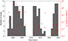 |
Fig. 1. Temporal distribution of the > 100 MeV proton events included in the catalogue (histogram). Red dots show the corresponding peak proton intensities (Ip) with uncertainties measured by SOHO/EPHIN, plotted against the secondary (right-hand) axis. |
2.2. SEP peak flux and fluence determination
The SOHO/EPHIN instrument measures particles (protons, electrons, and helium nuclei) across a wide energy range, from a few mega-electronvolts up to several hundred mega-electronvolts. It provides consistent peak flux and fluence estimates as long as only count rates of the previously unused ERNE penetrating-particle counter are available. A detailed description of the SOHO/EPHIN high-energy proton measurements is given in Appendix B. Note that we strictly speaking provide only a > 100 MeV channel proxy that is described as a differential channel.
Mathematically, the integral flux of energetic particles above a given threshold energy, Eth, in a SEP event, here Eth = 100 MeV, is defined as the energy integral of the differential particle flux over all energies exceeding this threshold. If j(E) denotes the differential flux (e.g. in units of particles per square centimetre per second per steradian per mega-electronvolts), the corresponding integral flux J(> Eth) is given by
where Eth and Emax denote the threshold and maximum energy considered, respectively. While Eth = 100 MeV, Emax is based on the maximum proton energy obtained during each event. Note that for most GLEs the energy is above the maximum energy of EPHIN (EEPHIN ≈ 500 MeV) can measure.
In order to be consistent with the ERNE observations, the present analysis derives the integral flux only from a single broad energy channel rather than from multiple discrete energy bins. To characterise the effective energy response of this channel and to determine a representative mean energy, the bow-tie method is applied (for details see Appendix B). This approach combines the instrument response with assumed spectral shapes, here power laws with indices γ ∈ { − 5, −2} to define an effective energy and an associated geometric factor (see Equation (B.1) in the Appendix B). The resulting quantity is a differential channel and is therefore only a proxy for the integral particle flux with energies above E > 100 MeV. The uncertainty of the EPHIN measurements can be divided into statistical and systematic uncertainties. The systematic uncertainty is estimated to be of the order of 20%. The statistical uncertainties are determined by the Poisson statistic of the number of selected counts available that are measured in the energy loss interval of interest and vary between a few tens to about 1000 per hour (see Fig. B.1). Note that, with respect to the on-board data processing: the statistical error for large events can be larger than that for small events. However, for SEP events, additional factors have to be taken into account for the systematic error, so that in what follows, only the statistical error is provided. Note, the derived proxy fluxes are not directly comparable with energetic particle measurements from the GOES satellites, which are provided primarily as integral flux channels above a certain energy threshold (e.g. > 100 MeV). For details, see Bruno (2017), Kress et al. (2021), and references therein.
The > 100 MeV proton flux derived from EPHIN measurements is averaged over one-hour intervals to ensure sufficient counting statistics. Onset times are taken from ERNE measurements, and the same background intervals as those used for ERNE are applied. The peak flux is defined as the maximum hourly value within the first few hours after the onset. The fluence is computed by integrating the particle flux from the onset until it decreases to 50–10% of the peak value or falls below 3σ–5σ above the background level. A figure illustrating this procedure is shown in Appendix B.
A so-called low-energy-loss statistics (LELS) issue occurs when the EPHIN energy-loss buffer becomes dominated by low-energy particles, leaving too few counts at higher energies (e.g. > 50 MeV protons) for reliable flux estimation. The priority scheme was modified in 2022, which has improved the high-energy statistics since then. Another limitation arises during SOHO keyhole periods (KHPs) – intervals typically lasting from a few days to two weeks, when telemetry is reduced or interrupted due to antenna pointing constraints. These periods occur once or twice a year at predictable times, determined by the spacecraft’s orbital geometry relative to Earth and the Sun, and can lead to data gaps or degraded measurements.
Figure B.7 in Appendix B shows two examples of data limitations affecting the > 100 MeV proton proxy from SOHO/EPHIN. The published dataset provides, for each event, the background level, peak flux, fluence, and the end date used for the fluence integration. Events affected by LELS or keyhole periods (respectively, 53 and 18), are indicated with the labels ‘lels’ and ‘khp’ in the dedicated ‘comments’ column. Figure 2 summarises the catalogue statistics for the SOHO/EPHIN peak intensities and fluences.
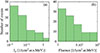 |
Fig. 2. Distributions of > 100 MeV proton peak intensities (panel (a)) and fluences (panel (b)) measured by SOHO/EPHIN for 107 and 97 events of the catalogue, respectively. |
3. Solar associations
The electromagnetic characteristics of the candidate solar sources provide key information on SEP acceleration and transport from the Sun to the point of in-situ measurement. Solar associations of the identified SEP events were established through inspection of all available observations, and cross-checked against published catalogues: (1) GOES > 10 MeV protons2, (2) Cane et al. (2010), (3) Richardson et al. (2014), and (4) Paassilta et al. (2017). For events with no ERNE or EPHIN onset determined, onsets were searched in other high-energy datasets, such as STEREO/In-situ Measurements of Particles and CME Transients (IMPACT)/High Energy Telescope (HET) and the GOES/Space Environment Monitor (SEM)/Energetic Particles Sensor (EPS) data (from SEPEM dataset). When required, lower-energy channels were examined, bearing in mind their slower particle propagation.
Only one event showed neither a CME nor a soft X-ray flare; all others exhibited at least one of these solar signatures. In total, 73% of confirmed SEP events (125/172) have clear associations with both a flare and a CME. For 22 events, multiple potential solar sources were identified; the selected one is reported in the catalogue, while alternatives and differences with published catalogues are noted in the ‘general notes’ (Appendix C). Figure 3 illustrates, for one representative > 100 MeV SEP event, the various solar signatures considered in this work – proton flux, flare emissions, radio and CME signatures, and GLEs. Dates in the catalogue follow the ISO 8601 format (yyyy-MM-ddTHH:mm:ssZ), where the trailing Z indicates UTC time. Each group of columns includes a comments field providing additional relevant information. The detailed catalogue structure is described in Appendix C.
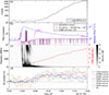 |
Fig. 3. Representative example of the solar associations for the 28 October 2021 > 100 MeV SEP event (No 137) corresponding to GLE73. Panel (a): ERNE proton counts at > 100 MeV. Panel (b): Soft X-ray flux (1–8 Å, GOES, blue) and high-energy flare emissions, including hard X-rays (Solar Orbiter/STIX, 4–10 keV, purple) and γ-rays (Fermi/LAT, > 100 MeV flux, pink). Panel (c): Radio dynamic spectrum (e.g. Wind/WAVES) with over-plotted CME height–time profile from coronagraph observations (SOHO/LASCO). Panel (d): Ground-level neutron monitor data showing relativistic particle increases. |
3.1. Identification of soft X-ray flares
Soft X-ray (SXR) enhancements are observed during solar flares, one of the two main accelerators of SEPs. SXR flare intensity correlates with CME speed and shock strength (Salas-Matamoros & Klein 2015; Jarry et al. 2023; Papaioannou et al. 2024), and with SEP event intensity (e.g. Papaioannou et al. 2016; Kouloumvakos et al. 2019). Strong flares are typically linked to fast, wide CMEs and intense SEP events.
To identify SXR flare associations, the solar particle release (SPR) time was estimated using the IRAP Propagation Tool (Rouillard et al. 2017) in ‘SEP propagation mode’. Assuming scatter-free propagation along the Parker spiral, the tool provides the solar footpoint and SPR time based on in-situ solar wind speed. Candidate flares were then searched around or before this time within the active-region belt. SXR fluxes were obtained from the GOES X-ray Sensor (XRS)3, operating since 1975 under NOAA (Woods et al. 2024). The 1–8 Å channel defines the standard flare classification (A–X classes for fluxes of 10n W m−2, n = [–8…–4]). Following Hudson et al. (2024) and the reprocessed science-quality data from NOAA National Centers for Environmental Information (NCEI), a calibration factor of 1.43 was applied to the GOES-1 through GOES-15 SXR datasets. Data cadence ranges from 1 min (GOES 8–12) to 1–2 s (GOES 13–18). For each SEP event, the most intense flare within the derived window was selected. Ambiguous cases with multiple nearby flares were reviewed individually, and alternatives are noted in the catalogue comments. Events with flares located behind the solar limb were marked as ‘far side’ and excluded from flare analysis (41/172 events). An example of GOES SXR flux is shown in panel (b) of Figure 3. Flare start, peak, and end times, as well as Hα locations, were taken from the GOES catalogues4. For events after October 2002, locations were verified and completed using Solar Dynamics Observatory (SDO)/Atmospheric Imaging Assembly (AIA) EUV observations from SolarSoft5. Discrepancies between catalogues occurred in only three cases (Events 103, 113, and 120), for which SolarSoft values were adopted. One remaining case (Event 18) was completed using Cane et al. (2010). SXR peak fluxes were extracted from GOES time series6. Fluences were obtained by trapezoidal integration between the reported start and end times. The catalogue specifies the GOES spacecraft used (‘Observer’ column) and provides SolarSoft links and positional remarks in the comments (‘behind the limb’ or ‘far side’). Overall, 131 of 172 SEP events (76%) were clearly associated with an SXR flare, while 41 were far-side events. Figure 4 shows the distribution of flare peak intensities, longitudes, rise times, and durations. Flare longitudes range from −89° to 132°, with a mean (median) of 49.9° (54.5°), whereas latitudes range from −37° to 30°, with a mean (median) of −1.2° (−4°). The predominance of western flares, and the low dispersion of latitudes around the equator, indicates the importance of an optimal magnetic connection of the source to Earth for > 100 MeV detections. SXR peak fluxes span 2.5 × 10⁻⁶–2.8 × 10⁻³ W m−2, with a mean of 2.8 × 10⁻⁴ W m−2 and a median of 1.1 × 10⁻⁴ W m−2, confirming that strong SEP events are primarily associated with strong (> M-class) flares.
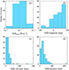 |
Fig. 4. Statistics of the identified soft X-ray flares associated with > 100 MeV SEP events (131/172, 76%). From left to right: SXR peak flux, flare longitude in Stonyhurst co-ordinates, rise time (peak minus start time), and total duration. |
3.2. Identification of hard X-rays
Hard X-ray (HXR) observations provide key diagnostics of flare-accelerated electrons and the hottest plasma components. Unlike SXRs, mainly produced by ∼10–30 MK thermal plasma (see Sect. 3.1), HXRs are dominated by bremsstrahlung emission from non-thermal electrons, i.e from energetic electrons colliding with ambient protons, with a thermal contribution at the lower energies from plasma hotter than ∼30 MK. The strongest signatures of particle acceleration appear during the impulsive phase, typically as bursts of HXR and microwave emission, both tracing non-thermal electron populations (see e.g. Klein 2021a).
HXR flare associations were established from two complementary instruments. RHESSI (2002–2018) provided HXR and γ-ray measurements from 3 keV to 20 MeV, while the Spectrometer Telescope for Imaging X-rays (STIX) on board Solar Orbiter (SO) has operated since 2020, offering HXR imaging spectroscopy between 4–150 keV. For events 43–134, both RHESSI time series (retrieved from the RHESSI data browser7) and the RHESSI flare catalogue8 provided by NASA were used. This catalogue lists detections in the 6–12 keV range, providing start, end, and peak times, as well as peak and total counts. For events 135–172, analysis relied on the SO/STIX time series from the STIX data browser9 and its science flare list10, based on detections in the 4–10 keV band. Note that RHESSI and STIX counts correspond to different energy ranges and response matrices; therefore, peak intensities are not directly comparable across instruments. Associations between > 100 MeV SEP events and HXR flares were established by comparing flare timing in hard and soft X-rays. Only HXR flares peaking after the SXR onset (±1 min) and no later than 30 min after the SXR peak were retained, consistent with the Neupert effect (Neupert 1968), which links impulsive HXR emission to the subsequent rise of SXR emission. A few exceptions were made: for SEP event 50 (22 August 2002), the nearest HXR flare was spatially distinct from the SXR source, so the preceding co-located flare was selected instead; for event 152 (17 July 2023), the HXR peak occurred 10 min before the SXR onset but overlapped in duration and was particularly intense; for events 81 (7 September 2005) and 119 (7 January 2014), HXR peaks occurred 40–42 min after their SXR peaks. Solar Orbiter catalogues, namely the Solar Orbiter’s Comprehensive Solar Energetic Electron event Catalogue (CoSEE-Cat; Warmuth et al. 2025) and the Solar Orbiter large SEP events catalogue (Papaioannou et al., in prep.), were also used to cross-check STIX associations. Because RHESSI and STIX provide limited coverage restricted to their operational periods and visible disc, occulted flares may be only partially or not at all detected. For each event, we list the start, peak, and end times, peak and total counts, maximum energy range, flare location in Carrington co-ordinates, and the observing spacecraft. A comment column indicates whether the flare was on the far side or behind the limb. Far-side events were not observed, while behind-the-limb events were measured but not positioned, and possibly occulted. Among the events for which an HXR search was possible (No. 43–172, as the first 42 precede RHESSI), 19% (25/130) were far side and 4% (5/130) lacked RHESSI data. Figure 5 summarises the measured HXR peak intensities, fluences, rise times, and durations. The mean HXR magnitude is 8.2 × 10⁵ counts, ranging from 23 to 1.6 × 10⁷ counts, with a median of 5.9 × 10⁴ counts.
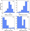 |
Fig. 5. Statistics of the identified hard X-ray flaring sources for the > 100 MeV catalogue (76%, 131/172 events). From left to right: distribution of HXR peak intensity, flare fluence (in counts), rise time (HXR peak – start), and total duration. |
3.3. Identification of type III radio bursts
Radio bursts are classified into five categories (types I–V) based on their frequency–time spectrograms (Wild et al. 1963). Type III bursts are the most common coherent solar radio emissions, produced by beams of flare-accelerated electrons (tens to hundreds of kilo-electronvolts) escaping along open magnetic field lines into the interplanetary (IP) medium (Reid & Vilmer 2017). Their rapid frequency drift reflects electron propagation through progressively less dense plasma, generating emission at the local plasma frequency and its harmonic. They often occur in groups during major solar eruptions, indicating successive magnetic reconnection episodes (see panel (c) of Fig. 3). Using coronal density models, the timing of a type III burst can therefore constrain the release time and coronal height of the associated SEP event.
The search for type III associations combined space- and ground-based radio observations to ensure full spectral and temporal coverage. Ground-based instruments typically observe from ∼10 MHz to a few gigahertz, while lower frequencies are blocked by the ionosphere. We used data from observatories worldwide covering 10 MHz–2.5 GHz, including stations in Australia, the USA, Japan, Greece, and France. Space-based receivers, Wind/WAVES and the twin STEREO/WAVES instruments (Bougeret et al. 2008), extend the coverage to kilohertz–megahertz frequencies originating in the outer corona and IP medium. All instruments used for identifying radio signatures of the SEP events are summarised in Appendix E. Type III bursts were identified by their temporal association with the start and peak times of the parent SXR flare. For far-side events, the timing was instead compared with the CME onset or any corresponding type II burst (see Section 3.4). Spectra from WIND/WAVES11 and STEREO/WAVES12 were visually inspected to determine the associated type III start time and frequency range, and this informations was reported in the catalogue along with the observing instrument(s) (SWAVES and/or WAVES). Ground-based identifications were obtained from compiled NOAA13 and SolarMonitor14 reports, which include observations from the Radio Solar Telescope Network (RSTN) and other stations. When available, event lists from the e-Callisto network15 and composite dynamic spectra from the LESIA Radio Monitoring service16 were also examined. For ground-based detections, we recorded the observing station(s), start time, and full frequency range; when multiple stations reported the event, the earliest start time and the minimum–maximum frequency limits across all reports were adopted. Type III radio bursts were identified for all (100%) SEP events in the catalogue, although some were detected only from space or from the ground. All associations were cross-checked with published catalogues, and matching identifications are noted in the type III comments. The referenced catalogues are Papaioannou et al. (2016), covering 1998–2013, and Kouloumvakos (2017), spanning 1997–2010.
3.4. Identification of type II radio bursts
Type II radio bursts trace shock waves accelerating particles in the solar atmosphere, typically driven by fast CMEs whose speeds exceed the local Alfvén speed (Kumari et al. 2023, and references therein), and less frequently by termination shocks from powerful flares (Hillaris et al. 2006). Such shocks are strong candidates for producing very high-energy SEPs (Klein 2021b). In dynamic spectra, type II bursts appear as slowly drifting, narrowband emissions reflecting the decreasing plasma density as the shock moves outwards. They are usually identified by visual inspection since they often occur close in time to other emissions (type III or IV). Ground-based observations commonly show a rapidly drifting type III burst (flare electrons) followed by the slower type II emission (shock vicinity), while space-based measurements usually provide a clearer separation as electron beams propagate faster than the shock. Morphological characteristics depend on the shock strength and ambient plasma conditions (Wild et al. 1963), making type II bursts valuable diagnostics of shock dynamics and particle acceleration regions tracing.
Type II associations for SEP events were retrieved from the same space- and ground-based instruments used for type III identifications (Sect. 3.3), ensuring broad spectral and temporal coverage of this study to trace shocks from the low corona to the IP medium. Associations were based on CME release times. Type II bursts were identified by visual inspection using standard criteria based on their slow drift rate (as compared to type III bursts), harmonic structure (fundamental and second harmonic emission lanes), and morphology which sometimes exhibits fragmented or ‘herringbone’ structure. Quantitative thresholds, for example on minimum burst duration or signal-to-noise ratio were not applied. For each identified type II burst in space-borne spectra we recorded the observing instrument (SWAVES and/or WAVES), start time, and frequency range. Additional information was taken from the multi-vantage-point type II catalogue17 of Mohan et al. (2024b). Ground-based detections were catalogued with observing station(s), start time, and frequency range; when multiple stations reported the event, we recorded all of them, the earliest start time, and the minimum–maximum frequencies observed. Positive type II identifications were established for most SEP events (163/172, i.e. 95%), cross-checked with several published catalogues: the continuously updated Gopalswamy et al. (2019)18 list (1996–2024), Papaioannou et al. (2016) (1998–2013), and Kouloumvakos (2017), covering 1997–2010.
3.5. Identification of type IV radio bursts
Type IV radio bursts appear as broadband continuum emissions in dynamic spectra, generally linked to major flares or CMEs (Kahler 1992). They are classified as moving or stationary depending on whether a clear frequency drift is observed. In the context of SEP events, type IV bursts trace prolonged electron acceleration and trapping in coronal magnetic structures, complementing X-ray and coronagraph data in characterising the timing and nature of acceleration sites (Mohan et al. 2024a).
Space-based type IV associations were obtained directly from the Mohan et al. (2024a)19 catalogue, which uses Wind/WAVES and both STEREO/WAVES (Ahead and Behind) observations. For each associated event, we list the observing spacecraft, onset time, duration (in minutes), and end frequency (in megahertz). Complementary ground-based detections were retrieved from the sources described in Sect. 3.3 and Appendix E, with the corresponding station(s), start time, and frequency range included in the catalogue. Type IV radio bursts were identified for 53% of the events (91/172). Their detection remains challenging due to variable spectral morphologies, frequent overlap with type II and type III emissions, and gaps in instrumental frequency coverage. These factors likely contribute to the relatively low association rate derived in this study.
3.6. Identification of γ-ray emissions
Observations of solar γ-rays and neutrons provide direct diagnostics of high-energy ions accelerated during eruptions. These ions interact with the lower solar atmosphere, producing γ-ray emission through nuclear reactions (Vilmer et al. 2011). Ions in the 1–100 MeV/nuc range generate line emissions from nuclear de-excitation, neutron capture, and positron annihilation, while energies above 100 MeV/nuc are dominated by neutral pion decay. Solar γ-ray emission typically exhibits two phases (Frost & Dennis 1971): a prompt component coinciding with the flare, and a delayed, prolonged component that persists well after the impulsive flare signatures have faded (Akimov et al. 1991; Ryan 2000; Rank et al. 2001). It is generally accepted that the first component is linked to ion acceleration in the reconnection region, whereas the origin of the delayed phase remains unresolved and actively debated. Proposed scenarios include continuous acceleration or trapping in large coronal structures (e.g. Ryan 2000; Grechnev et al. 2018; de Nolfo et al. 2019; Bruno et al. 2023), as well as acceleration at CME-driven shocks (e.g. Ackermann et al. 2014; Share et al. 2018). Durations of sustained γ-ray events correlate with those of > 100 MeV SEP events, though the latter are usually about five times longer (Share et al. 2018). Fermi/Large Area Telescope (LAT) has observed γ-ray emission from behind-the-limb flares (Ackermann et al. 2017), demonstrating that pion-decay γ-rays can originate tens of degrees from the active region (Plotnikov et al. 2017). Although correlations with SEP events and CME properties are often reported, notable counterexamples and strong event-to-event variability indicate that these relationships are not universal, and that sustained γ-ray emission cannot be explained by a single acceleration mechanism. The Fermi space telescope and its two main instruments provide systematic detection of these two phases since 2011. The LAT detects photons from 30 MeV to > 300 GeV (Lange & Pohl 2013; Ajello et al. 2021a), while the Gamma-ray Burst Monitor (GBM) covers a few kilo-electronvolts to ∼30 MeV (Meegan et al. 2009), bridging low-energy X-rays and high-energy γ-rays.
We analysed publicly available GBM20 data for SEP events 87–172 (2011–2024), corresponding to the Fermi mission period, to establish SEP–γ-ray associations by temporal correspondence with sustained emission periods, with no ambiguous overlaps. The Fermi/LAT Significant Event List21 (> 100 MeV) and Fermi-LAT Solar Flare Catalog (30 MeV–10 GeV, Ajello et al. 2021b) were also inspected over the same periods. An example of a Fermi/LAT light curve is shown in panel (b) of Fig. 3. For each associated event, the catalogue lists from Fermi/GBM the onset, peak, and end times, peak intensity (counts s−1), total counts, and observing instrument, with comments noting missing Fermi data or flare absence. Among the 87 SEP events occurring during the Fermi era, 65 (75%) show associated γ-ray emission. Non-detections may result from insufficient proton energies (> 300 MeV required for pion decay), Fermi’s orbital night-time gaps, or far-side eruptions magnetically disconnected from the visible disc.
3.7. Identification of coronal mass ejections (CMEs)
Coronal mass ejections are sudden large-scale releases of plasma ejected into the upper corona and the solar wind. They result from the reconfiguration of coronal magnetic fields through various processes and strong ones often accompany flares or prominence eruptions (Yashiro et al. 2005). Fast and wide CMEs represent key components of major solar storms, typically involving (1) an initiation phase with flaring or prominence activity, (2) coronal expansion possibly driving shocks and large-scale solar atmosphere disturbances, and (3) the ejection of mass and magnetic flux into interplanetary space. When a CME appears as a halo-like enhancement around the coronagraph’s occulting disc, it is classified as a halo CME (see Webb & Howard 2012, and references therein).
Associations between SEP events and CMEs were determined using LASCO C2 and C3 coronagraphs on board SOHO, which have continuously monitored the solar corona since 1996. All manually identified CMEs from these instruments are compiled in the SOHO/LASCO CME catalogue (Gopalswamy et al. 2009), available at the CDAW Data Center22. Coronal mass ejection linear speeds were derived from first-order polynomial fits to height–time measurements (see panel (c) of Fig. 3) listed in that catalogue. For each SEP event, CMEs occurring after the onset of the associated SXR flare (Sect. 3.1) were considered; in the absence of recorded SXR data, the SEP onset time was used instead. Given the high energies of > 100 MeV SEP events, their CMEs are generally fast and well defined in LASCO observations, although some events coincide with LASCO data gaps, explicitly flagged in the catalogue. For each CME, the catalogue lists the first LASCO C2 appearance time, linear speed, angular width, and a direct link to the corresponding movie in the LASCO database. Coronal mass ejections with apparent widths of 360° are identified as halos. Associations were found for 96% (165/172) of SEP events; the remaining cases correspond to SOHO/LASCO data gaps, noted as ‘NO DATA’ in the source field. Figure 6 summarises CME kinematics for > 100 MeV proton events. Coronal mass ejection speeds range from 448 to 3387 km s−1, with a median of 1336 km s−1 and a mean of 1404 km s−1. Widths span from 76° to 360°, with mean and median values of 331° and 360°, respectively. These statistics confirm that strong SEP events are predominantly associated with fast, halo CMEs (see e.g. Papaioannou et al. 2016, and references therein).
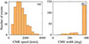 |
Fig. 6. Statistics on the CMEs associated with the > 100 MeV events (96%, 162/169 events). Panel (a): CME speed distribution (kilometre per second). Panel (b): CME width distribution (deg). |
3.8. Identification of ground-level enhancements (GLEs)
Ground-Level Enhancements are rare, high-intensity SEP events in which protons reach relativistic energies (up to the GeV range) and penetrate the Earth’s atmosphere, producing secondary particle cascades detected by ground-based neutron monitors worldwide (Gopalswamy et al. 2012; Papaioannou 2023). A GLE is defined as a near-simultaneous increase in at least two neutron monitors, including one near sea level, while events detected only at high-altitude stations are termed sub-GLEs (Poluianov et al. 2017). Representing the most energetic end of the SEP spectrum over the past seven decades, GLEs provide unique diagnostics of extreme particle acceleration at the Sun (Kocharov et al. 2023). Their properties (Asvestari et al. 2017) have been used to analyse extreme SEP events (Usoskin et al. 2023) and to quantify their impact on the solar radiation environment (Herbst & Papaioannou 2025). GLEs are generally associated with powerful flares and fast CMEs driving strong shocks (see e.g. Mishev et al. 2021, 2022, 2024, and references therein), but their occurrence is also favoured by good magnetic connectivity and by the presence or interaction of transient solar-wind structures–such as ICMEs, magnetic clouds, and shocks (Rouillard et al. 2012; Papaioannou et al. 2016; Lario et al. 2017), making them particularly complex to fully understand (Cliver 2006).
GLE and sub-GLE associations were identified manually using the neutron monitor database23. For each event, the catalogue lists the maximum intensity, the observing station, and the GLE identifier (or ‘sub-GLE’ label). When available, fluences from Usoskin et al. (2020) are also included. The catalogue contains 18 GLEs and 4 sub-GLEs. All GLEs and sub-GLEs observed during the studied period are represented, except GLEs 58, 60, and 61, which are absent due to SOHO/ERNE data gaps. Fluence values were taken by Usoskin et al. (2020) who derive full-event, de-trended, time-integrated NM intensities that include both the early anisotropic and later isotropic phases. Thus, unlike first-hour–focused inversions, their reported values represent the total omnidirectional fluence. These are available for 11 of the 22 recorded events.
4. Results
Table 1 summarises the principal statistical properties of the > 100 MeV events and their solar associations. Where data exist, every SEP event is associated with a CME and a SXR flare, implying particle acceleration by the flare, the CME-driven shock, or both. Median CME speeds exceed 1300 km s−1 and median CME angular widths are ∼360° (Table 1).
Median and mean values with standard deviations (σ) of the parameters characterising the > 100 MeV proton events and the associated CMEs, soft and hard X-ray flares, and γ-ray emissions.
The typical travel time of 100 MeV protons is 19–49 min depending on the path length (1–2.5 AU). Including light-travel delays, the observed particle onset should therefore occur within roughly one hour of its parent solar signature. Figure 7 presents timing differences between SEP release times (from ERNE onset) and associated solar signatures (CME, SXR, HXR, type II/III/IV, γ), shown for two travel-time assumptions (short and long). Table D.1 (Appendix D) gives counts of positive and negative delays under both assumptions. Notably, ∼21% (25/121; short travel) and ∼19% (23/121; long travel) of SEPs occur during the impulsive flare phase (after SXR onset but before SXR peak) (Benz 1993), while ∼35% (43/121) and ∼41% (50/121) occur during the SXR decay, indicating substantial late or extended acceleration. Seven events show extreme delays (> 360 min); these are listed in Appendix D.
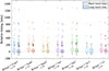 |
Fig. 7. Distribution of the SEP events with respect to timing differences (in minutes) between the > 100 MeV proton events release times determined with SOHO/ERNE SEP onset and the associated solar signatures onsets. Two travel-time assumptions are considered: short (light colours) and long (dark colours) path lengths, respectively, 1 and 2.5 AU. Solar signatures are shifted to the solar time according to the light travel time, and are, from left to right: CME first appearance in SOHO/LASCO coronographs (blue), soft X-ray onset time (red), hard X-ray onset time (yellow), type II radio burst onset time (purple), type III radio burst onset time (green), type IV radio burst onset time (cyan), gamma ray burst onset time (pink). In each boxplot, the middle line indicates the median of the distribution whereas the top of bottom edges of a box are the upper and lower quartiles, respectively. Outliers are values that are more than 1.5 times the distance between the top and bottom edges. The number of events considered in each boxplot is indicated in the x axis. |
Timing between solar associations is shown in Fig. 8. Type IV bursts consistently follow SXR onset and typically occur after type III bursts. Coronal mass ejection first appearances and type II onsets are tightly clustered around zero delay, consistent with CME-driven shocks as the type II source, although individual discrepancies up to ∼1.5 h exist.
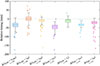 |
Fig. 8. Same as Figure 7 for the timing difference between solar associations in minutes. From left to right, comparisons between: soft X-ray onset time (tSXR) and CME first appearance in SOHO/LASCO coronographs (tCME) (blue) ; tCME and type II radio burst onset time (ttII) (red) ; tSXR and type III radio burst onset time (ttIII) (yellow) ; tSXR and type IV radio burst onset time (ttIV) (purple) ; tSXR and gamma ray burst onset time (tγ) (green) ; ttIII and ttIV (cyan) ; ttIII and ttII (pink). |
Two notable exceptions appear in the timing distributions. Event 72 (17 January 2005) exhibits an unusually long SXR rising phase of about three hours, leading to a CME first appearance in LASCO which occurs few minutes (< 6 min) before the SXR onset. This event is also visible in the Δ(tSXR, onset − tHXR, onset) distribution in Fig. 9 panel (a). There is a strong tendency for SXR onset to precede HXR one, consistent with Veronig et al. (2002b), who found this behaviour in 92% of events. Event 104, on the other hand, shows a delayed SXR peak occurring ∼3.5 h after the CME first appearance and the other solar signatures, likely due to a second, overlapping flare episode. It appears as an isolated point in Δ(tSXR − ttIII) and Δ(tSXR − ttIV) distributions (Fig. 8). Apart from these two cases, SXR and HXR peak times generally agree within 50 min, reflecting their close physical connection during the impulsive phase of energy release.
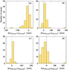 |
Fig. 9. Timing difference (hours in UT) between soft and hard X-rays. |
Figure 10 compares HXR and SXR peak intensities using separate RHESSI and SO/STIX samples (see Sect. 3.2). In this and all subsequent bi-logarithmic figures, the reported correlation coefficients and regression lines are obtained from log–log linear fits. Power-law fits yield
 (1)
(1)
 (2)
(2)
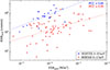 |
Fig. 10. Hard X-ray peak intensity in counts/s from RHESSI (red points) and Solar orbiter/STIX (blue points) as a function of soft X-ray peak intensity in W/m2 from GOES. The PCC of the respective best fits (red and blue lines) are indicated in the legend. |
with Pearson correlation coefficients (PCCs) of 0.50 (N = 65, p = 2.8 × 10⁻⁵, 95% confidence interval (CI) [0.28,0.66]) for RHESSI and 0.68 (N = 25, p = 2.8 × 10⁻⁴, 95% CI [0.37,0.85]) for SO/STIX. These results are comparable to earlier studies Veronig et al. (e.g. 2002a, PCC = 0.57). However, correlation between SXR peak and HXR fluence (not shown here) are weaker (PCC of 0.35 (N = 64, p = 4.1 × 10⁻³, 95% CI [0.11, 0.55]) and 0.46 (N = 23, p = 2.6 × 10⁻², 95% CI [0.06, 0.73]), respectively), compared to the 0.71 obtain by Veronig et al. (2002a).
Figure 11 shows CME speed versus SXR peak flux. For our catalogue:
 (3)
(3)
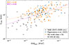 |
Fig. 11. Coronal mass ejection speed from SOHO/LASCO as a function of the soft X-ray peak from GOES, for 49 events studied in Salas-Matamoros & Klein (2015) (grey), 65 SEP events that reach E > 100 MeV studied by Papaioannou et al. (2023) (blue), and 124 events from the present catalogue (orange). Power law fits for our sample and the combined three are lines in orange and pink, respectively. |
with PCC = 0.40 (N = 124, p = 3.3 × 10⁻⁶, 95% CI [0.25, 0.54]). Combining our sample with literature datasets (i.e. Salas-Matamoros & Klein 2015; Papaioannou et al. 2023) yields
 (4)
(4)
with PCC = 0.60 (N = 238, p = 6.1 × 10⁻²², 95% CI [0.50, 0.68]). These results are in agreement with previous studies that reported PCC of 0.43 (Papaioannou et al. 2024) and 0.48 (Salas-Matamoros & Klein 2015) and within the range of 0.37 and 0.50 that has been identified in E > 10 MeV SEPs (Yashiro & Gopalswamy 2009) and GLEs (Gopalswamy et al. 2012), respectively. The modest correlation indicates that, although flares and CMEs share a common origin in the large-scale reconfiguration of the coronal magnetic field and therefore do not occur in isolation (see the relevant discussion in Papaioannou et al. 2025b), CME kinematics are governed by additional factors. In particular, the CME speed is strongly modulated by the properties of the ambient coronal environment and by the reconnection dynamics that drive energy release. Consequently, the soft X-ray flux, while a useful proxy for flare intensity, cannot by itself provide a substitute of the CME speed. Furthermore, it is evident that the related SXR fluxes and the corresponding CME speeds across all samples at E > 100 MeV in Fig. 11 (orange and blue points) indicate that such high-energy SEP events are associated with strong flares and fast CMEs. Given our pre-selection of highly energetic events, it is normal to observe a shift of the spread relative to the Salas-Matamoros & Klein (2015) sample (black points).
Proton peak intensities (> 100 MeV, EPHIN) correlate moderately with SXR peak flux (Fig. 12; PCC = 0.48 (N = 84, p = 4.6 × 10⁻⁶, 95% CI [0.29, 0.63])), consistent with the 0.49 reported by Papaioannou et al. (2016). Restricting to magnetically well-connected longitudes (20°–87°, following Belov et al. (2005)) yields PCC = 0.44 (N = 49, p = 1.8 × 10⁻³, 95% CI [0.18, 0.64]), showing that improved nominal connection does not substantially strengthen the SXR–SEP relation which remains moderate. For a given flare magnitude, the peak proton flux measured by SOHO varies by over four orders of magnitude, highlighting the large intrinsic variability of SEP events and the need for multiple parameters to explain the underlying physical processes. This scatter suggest that SXR flux alone cannot account for the observed SEP variability; CME kinematics, shock acceleration efficiency and interplanetary transport effects likely contribute significantly. The higher PCC (0.66) reported by Belov (2017) under similar longitudinal conditions likely reflects differences in sample definition and size. The substantial scatter in both datasets introduces statistical noise that can weaken the apparent correlation strength.
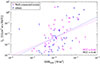 |
Fig. 12. SOHO/EPHIN proton peak intensity > 100 MeV (Ip) with uncertainties as a function of the soft X-ray peak from GOES. Events considered as well connected, i.e with a SXR longitude between 20 and 87 degrees, are shown in pink. Pearson correlation coefficients of well-connected and all events are, respectively, in pink and black. |
A somewhat stronger correlation is found between SEP peak flux and CME linear speed (Fig. 13):
 (5)
(5)
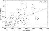 |
Fig. 13. SOHO/EPHIN proton peak intensity > 100 MeV (Ip) with uncertainties as a function of the linear CME speed measured with SOHO/LASCO (VCME). |
The obtained PCC of 0.54 (N = 106, p = 2.8 × 10⁻⁹, 95% CI [0.38, 0.66]) is stronger than the ∼0.40 reported for E > 100 MeV events (Papaioannou et al. 2016, 2024), and weaker than the 0.71 found by Richardson et al. (2014) for 25 MeV protons. These trends align with Ameri et al. (2024), who showed that lower-energy SEPs (E < 100 MeV) are primarily CME-driven, while higher-energy particles (E > 100 MeV) likely originate from flare reconnection or low-coronal shock acceleration, possibly followed by re-acceleration at CME-driven shocks higher in the corona. These empirical correlations must also be considered in the context of the Big Flare Syndrome (BFS, Kahler 1982), whereby large eruptive events tend to produce strong signatures across many observables. The moderate SEP-SXR correlations, and even the stronger SEP–CME relationship, may partly reflect the overall event magnitude rather than direct causal links, so these results could be interpreted as statistical associations rather than strict evidence of causation.
Comparisons between GLEs and SEPs peak intensities are shown in Fig. 14. For 14 GLE and sub-GLE events, we find a moderate correlation (PCC = 0.47, p = 9.2 × 10⁻², 95% CI = [–0.08, 0.80]), weaker than the high-energy results of Waterfall et al. (2023) (0.879-0.925 at ∼340–730 MeV) and Oh et al. (2010) (0.867-0.874 at ∼380–700 MeV). Extending the comparison to fluences (11 events; Fig. 15) yields a stronger PCC of 0.76 (p = 1.1 × 10⁻², 95% CI = [0.24, 0.94]), confirming the clear relationship between high-energy SEP fluences and neutron monitor responses, consistent with earlier findings (Oh et al. 2010; Waterfall et al. 2023), and further reinforces the strong physical connection between space-based SEP measurements and ground-level enhancements.
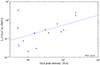 |
Fig. 14. SOHO/EPHIN proton peak intensity > 100 MeV (Ip) with uncertainties as a function of the integral GLE peak intensity (%.h) for 14 events of the present catalogue. |
5. Conclusion
We have compiled a comprehensive catalogue of SEP events with proton energies exceeding 100 MeV, based on a systematic search of SOHO/ERNE/HED penetrating-particle rates over May 1996–August 2024, as part of the SPEARHEAD project. The catalogue includes 172 SEP events and is currently available in Zenodo24 (Jarry et al. 2025). Peak fluxes and fluences were derived from SOHO/EPHIN data, whose recent recalibration enables reliable energy-resolved spectra above 100 MeV. The resulting dataset contains 172 events with complete information on their solar associations, including soft and hard X-rays, radio bursts of types II–IV, sustained > 100 MeV γ-ray emission, and CME signatures. Associations were found for nearly all events: 76% with SXR flares, 95% with type II bursts, 53% with type IV continua, 65 of 87 Fermi/LAT-era events with γ-rays, and 96% with CMEs – typically fast and wide, often halo CMEs.
The statistical analysis of temporal and energetic relationships between SEPs and their solar drivers reveals several key results:
-
The catalogue includes 172 events from 1996–2024, with near-complete coverage of CMEs, flares, and radio bursts, providing the most comprehensive reference to date for high-energy (> 100 MeV) SEP events observed by SOHO and enabling cross-calibration with other missions.
-
Timing analyses confirms that most > 100 MeV SEP releases occur shortly after X-ray onsets and CME first appearances (Fig. 7), indicating nearly simultaneous release of flare- and shock-accelerated particles. A few outliers (Appendix D) reveal complex multi-phase or overlapping eruptions, illustrating the diversity of acceleration scenarios.
-
Distributions of solar timing differences (Figs. 8, 9) show consistent sequencing: hard X-rays and type III bursts typically follow SXR onsets, confirming that impulsive acceleration is closely tied to early reconnection signatures.
-
The comparison of soft and hard X-ray timings and peaks (Figs. 9, 10) supports the Neupert effect, with SXR emission rising gradually after HXR impulsive phases. Correlations between their peak intensities (PCC = 0.50–0.68) confirm the expected impulsive–thermal coupling in major SEP-producing flares (Veronig et al. 2005).
-
The first appearance of a CME usually follows the SXR onset by 30–60 min, consistent with a shared magnetic restructuring. Correlations between CME speed and SXR peak flux remain moderate (Fig. 11, PCC = 0.4–0.6), in line with previous studies (Yashiro & Gopalswamy 2009; Salas-Matamoros & Klein 2015; Papaioannou et al. 2024), consistent with the idea that CME kinematics are influenced by both the flare energy release and other factors such as ambient coronal conditions and reconnection geometry.
-
Correlation between proton intensity and SXR peak flux remain moderate (Fig. 12), and the large scatter implies that SEP intensity is controlled by multiple factors beyond simple flare magnitude. The correlation with CME speed (Fig. 13, PCC = 0.54) is stronger than reported in previous high-energy studies (Papaioannou et al. 2016), but weaker than those found for lower-energy SEPs (Richardson et al. 2014). These empirical associations are consistent with scenarios in which both flare processes and CME-driven shocks contribute to > 100 MeV SEPs, although they may partly reflect overall event size (BFS) rather than a direct link. In addition, magnetic connectivity and pre-conditioning are important modifiers of high-energy SEP-event characteristics.
-
Comparisons between > 100 MeV SEPs and GLEs (Figs. 14–15) reveal a clear link between space- and ground-based measurements, with moderate correlation for peak fluxes (PCC = 0.47) and stronger for fluences (0.76), consistent with Oh et al. (2010), Waterfall et al. (2023). This confirms that the most energetic SEPs observed in space are the direct counterparts of GLEs.
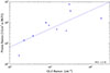 |
Fig. 15. SOHO/EPHIN proton fluence with uncertainties as a function of the omnidirectional integral GLE fluence expressed in cm−2 for 10 events of the present catalogue. |
Future developments of the catalogue are underway. The inclusion of CME observations from the STEREO/SECCHI suite (Howard et al. 2008) – particularly COR1, COR2, and HI imagery – will be consider as well as additional CME properties, such as de-projected speeds from the HELCATS catalogue25, to improve association accuracy and analysis. Complementary SXR observations from the MESSENGER X-Ray Spectrometer (Schlemm et al. 2007), when the spacecraft viewed the solar far side, and improved magnetic connectivity estimates using IRAP’s Magnetic Connectivity Tool (Rouillard et al. 2020), will further refine the association of SEPs with their solar sources.
High-energy SEPs (> 100 MeV) probe the most energetic regimes of particle acceleration associated with flares and CME-driven shocks. Associated with the more abundant lower-energy SEPs (E > 10 MeV), which provide essential and complementary constraints on acceleration and transport, sampling different parts of the particle spectrum and responding differently to shock strength, turbulence, and seed populations, these highest-energy particles offer additional diagnostic power. The rapid arrival of the earliest, prompt high-energy particles which have experienced less scattering preserve key information on acceleration timing and magnetic connectivity. Their close association with GLEs thus linked space-based SEP measurements to ground based observations. Given their rarity and strong association with the most powerful solar eruptions, high-energy SEP events serve as sensitive indicators of extreme solar activity. Combined with low-energy SEPs, their properties provide a more complete view of the physical conditions governing the most powerful solar events. By consolidating nearly three decades of observations into a single, uniformly processed catalogue, this work provides the most extensive reference dataset to date for investigating high-energy SEP origins, acceleration and propagation mechanisms, and to address many of the outstanding questions in SEP research.
Data availability
The complete catalogue created and used in this study is provided on https://zenodo.org/records/17520213. An interactive version of this catalogue is available at https://spearhead-he.eu/catalogues_hub?prefilter=soho100mev.
Acknowledgments
We thank the anonymous referee for their thorough and accurate review, which greatly improved the manuscript. This research received funding from the European Union’s Horizon Europe programme under grant agreement No 101135044 (SPEARHEAD) [https://spearhead-he.eu/]. Views and opinions expressed are, however, those of the author(s) only and do not necessarily reflect those of the European Union or the European Health and Digital Executive Agency (HaDEA). Neither the European Union nor the granting authority can be held responsible for them. B.H. and M.K. further acknowledge the support of the EPHIN and SEPT from the German Federal Ministry for Economic Affairs and Energy, the German Space Agency (Deutsches Zentrum für Luft- und Raumfahrt e.V., DLR) under grants 50OC2102, 50OC3202.
References
- Ackermann, M., Ajello, M., Albert, A., et al. 2014, ApJ, 787, 15 [NASA ADS] [CrossRef] [Google Scholar]
- Ackermann, M., Allafort, A., Baldini, L., et al. 2017, ApJ, 835, 219 [CrossRef] [Google Scholar]
- Agostinelli, S., Allison, J., Amako, K., et al. 2003, Nucl. Instrum. Methods Phys. Res. A, 506, 250 [Google Scholar]
- Ajello, M., Atwood, W. B., Axelsson, M., et al. 2021a, ApJS, 256, 12 [NASA ADS] [CrossRef] [Google Scholar]
- Ajello, M., Baldini, L., Bastieri, D., et al. 2021b, ApJS, 252, 13 [NASA ADS] [CrossRef] [Google Scholar]
- Akimov, V. V., Afanassyey, V. G., Belaousov, A. S., et al. 1991, Int. Cosm. Ray Conf., 3, 73 [Google Scholar]
- Ameri, D., Valtonen, E., Al-Sawad, A., & Vainio, R. 2024, Sol. Phys., 299, 133 [Google Scholar]
- Asvestari, E., Willamo, T., Gil, A., et al. 2017, Adv. Space Res., 60, 781 [NASA ADS] [CrossRef] [Google Scholar]
- Atwood, W. B., Abdo, A. A., Ackermann, M., et al. 2009, ApJ, 697, 1071 [CrossRef] [Google Scholar]
- Belov, A. V. 2017, Geomagn. Aeron., 57, 727 [NASA ADS] [CrossRef] [Google Scholar]
- Belov, A., Garcia, H., Kurt, V., Mavromichalaki, H., & Gerontidou, M. 2005, Sol. Phys., 229, 135 [NASA ADS] [CrossRef] [Google Scholar]
- Benz, A. O. 1993, Plasma Astrophysics: Kinetic Processes in Solar and Stellar Coronae (Dordrecht: Kluwer), 184 [Google Scholar]
- Bougeret, J. L., Kaiser, M. L., Kellogg, P. J., et al. 1995, Space Sci. Rev., 71, 231 [CrossRef] [Google Scholar]
- Bougeret, J. L., Goetz, K., Kaiser, M. L., et al. 2008, Space Sci. Rev., 136, 487 [CrossRef] [Google Scholar]
- Brueckner, G. E., Howard, R. A., Koomen, M. J., et al. 1995, Sol. Phys., 162, 357 [NASA ADS] [CrossRef] [Google Scholar]
- Bruno, A. 2017, arXiv e-prints [arXiv:1708.05641] [Google Scholar]
- Bruno, A., Bazilevskaya, G. A., Boezio, M., et al. 2018, ApJ, 862, 97 [Google Scholar]
- Bruno, A., de Nolfo, G. A., Ryan, J. M., Richardson, I. G., & Dalla, S. 2023, ApJ, 953, 187 [NASA ADS] [CrossRef] [Google Scholar]
- Cane, H. V., Richardson, I. G., & von Rosenvinge, T. T. 2010, Journal of Geophysical Research (Space Physics), 115, A08101 [Google Scholar]
- Cliver, E. W. 2006, ApJ, 639, 1206 [NASA ADS] [CrossRef] [Google Scholar]
- Cliver, E. W., Kahler, S. W., & Reames, D. V. 2004, ApJ, 605, 902 [NASA ADS] [CrossRef] [Google Scholar]
- de Nolfo, G. A., Bruno, A., Ryan, J. M., et al. 2019, ApJ, 879, 90 [NASA ADS] [CrossRef] [Google Scholar]
- Dierckxsens, M., Tziotziou, K., Dalla, S., et al. 2015, Sol. Phys., 290, 841 [CrossRef] [Google Scholar]
- Domingo, V., Fleck, B., & Poland, A. I. 1995, Sol. Phys., 162, 1 [Google Scholar]
- Dresing, N., Yli-Laurila, A., Valkila, S., et al. 2024, A&A, 687, A72 [NASA ADS] [CrossRef] [EDP Sciences] [Google Scholar]
- Dumbović, M., Kramarić, L., Benko, I., Heber, B., & Vršnak, B. 2024, A&A, 683, A168 [NASA ADS] [CrossRef] [EDP Sciences] [Google Scholar]
- Frost, K. J., & Dennis, B. R. 1971, ApJ, 165, 655 [Google Scholar]
- Gopalswamy, N., Yashiro, S., Michalek, G., et al. 2009, Earth Moon Planets, 104, 295 [NASA ADS] [CrossRef] [Google Scholar]
- Gopalswamy, N., Xie, H., Yashiro, S., et al. 2012, Space Sci. Rev., 171, 23 [NASA ADS] [CrossRef] [Google Scholar]
- Gopalswamy, N., Makela, P., & Yashiro, S. 2019, arXiv e-prints [arXiv:1912.07370] [Google Scholar]
- Grechnev, V. V., Kiselev, V. I., Kashapova, L. K., et al. 2018, Sol. Phys., 293, 133 [NASA ADS] [CrossRef] [Google Scholar]
- Hanser, F. A., & Sellers, F. B. 1996, SPIE Conf. Ser., 2812, 344 [NASA ADS] [Google Scholar]
- Herbst, K., & Papaioannou, A. 2025, A&A, 696, A63 [NASA ADS] [CrossRef] [EDP Sciences] [Google Scholar]
- Hillaris, A., Petousis, V., Mitsakou, E., et al. 2006, Adv. Space Res., 38, 1007 [Google Scholar]
- Howard, R. A., Moses, J. D., Vourlidas, A., et al. 2008, Space Sci. Rev., 136, 67 [NASA ADS] [CrossRef] [Google Scholar]
- Hudson, H., Cliver, E., White, S., et al. 2024, Sol. Phys., 299, 39 [NASA ADS] [CrossRef] [Google Scholar]
- Huttunen-Heikinmaa, K., Valtonen, E., & Laitinen, T. 2005, A&A, 442, 673 [NASA ADS] [CrossRef] [EDP Sciences] [Google Scholar]
- Jarry, M., Rouillard, A. P., Plotnikov, I., Kouloumvakos, A., & Warmuth, A. 2023, A&A, 672, A127 [NASA ADS] [CrossRef] [EDP Sciences] [Google Scholar]
- Jarry, M., Palmroos, C., Lavasa, E., et al. 2025, https://doi.org/10.5281/zenodo.17520214 [Google Scholar]
- Kahler, S. W. 1982, J. Geophys. Res., 87, 3439 [NASA ADS] [CrossRef] [Google Scholar]
- Kahler, S. W. 1992, ARA&A, 30, 113 [NASA ADS] [CrossRef] [Google Scholar]
- Kahler, S. W., Sheeley, N. R., Jr., Howard, R. A., et al. 1984, J. Geophys. Res., 89, 9683 [Google Scholar]
- Kaiser, M. L., Kucera, T. A., Davila, J. M., et al. 2008, Space Sci. Rev., 136, 5 [Google Scholar]
- Klein, K.-L. 2021a, Front. Astron. Space Sci., 7, 105 [NASA ADS] [Google Scholar]
- Klein, K.-L. 2021b, Front. Astron. Space Sci., 7, 93 [NASA ADS] [Google Scholar]
- Kocharov, L., Mishev, A., Riihonen, E., Vainio, R., & Usoskin, I. 2023, ApJ, 958, 122 [Google Scholar]
- Kouloumvakos, A. 2017, Ph.D. Thesis, University of Ioannina [Google Scholar]
- Kouloumvakos, A., Rouillard, A. P., Wu, Y., et al. 2019, ApJ, 876, 80 [NASA ADS] [CrossRef] [Google Scholar]
- Kress, B. T., Rodriguez, J. V., Boudouridis, A., et al. 2021, Space Weather, 19, e02750 [NASA ADS] [CrossRef] [Google Scholar]
- Krucker, S., Hurford, G. J., Grimm, O., et al. 2020, A&A, 642, A15 [NASA ADS] [CrossRef] [EDP Sciences] [Google Scholar]
- Kühl, P., & Heber, B. 2019, Space Weather, 17, 84 [CrossRef] [Google Scholar]
- Kühl, P., Banjac, S., Dresing, N., et al. 2015, A&A, 576, A120 [NASA ADS] [CrossRef] [EDP Sciences] [Google Scholar]
- Kühl, P., Gómez-Herrero, R., & Heber, B. 2016, Sol. Phys., 291, 965 [Google Scholar]
- Kühl, P., Dresing, N., Heber, B., & Klassen, A. 2017, Sol. Phys., 292, 10 [Google Scholar]
- Kühl, P., Heber, B., Gómez-Herrero, R., et al. 2020, J. Space Weather Space Clim., 10, 53 [CrossRef] [EDP Sciences] [Google Scholar]
- Kumari, A., Morosan, D. E., Kilpua, E. K. J., & Daei, F. 2023, A&A, 675, A102 [NASA ADS] [CrossRef] [EDP Sciences] [Google Scholar]
- Lange, J., & Pohl, M. 2013, A&A, 551, A89 [NASA ADS] [CrossRef] [EDP Sciences] [Google Scholar]
- Lario, D., Kwon, R.-Y., Riley, P., & Raouafi, N. E. 2017, ApJ, 847, 103 [NASA ADS] [CrossRef] [Google Scholar]
- Lin, R. P., Dennis, B. R., Hurford, G. J., et al. 2002, Sol. Phys., 210, 3 [Google Scholar]
- Mavromichalaki, H., Papaioannou, A., Plainaki, C., et al. 2011, Adv. Space Res., 47, 2210 [NASA ADS] [CrossRef] [Google Scholar]
- Meegan, C., Lichti, G., Bhat, P. N., et al. 2009, ApJ, 702, 791 [Google Scholar]
- Mewaldt, R. A., Looper, M. D., Cohen, C. M. S., et al. 2012, Space Sci. Rev., 171, 97 [Google Scholar]
- Mishev, A. L., Koldobskiy, S. A., Kocharov, L. G., & Usoskin, I. G. 2021, Sol. Phys., 296, 79 [NASA ADS] [CrossRef] [Google Scholar]
- Mishev, A. L., Kocharov, L. G., Koldobskiy, S. A., et al. 2022, Sol. Phys., 297, 88 [NASA ADS] [CrossRef] [Google Scholar]
- Mishev, A. L., Koldobskiy, S. A., Larsen, N., & Usoskin, I. G. 2024, Sol. Phys., 299, 24 [Google Scholar]
- Mohan, A., Gopalswamy, N., Kumari, A., Akiyama, S., & G, S. 2024a, ApJ, 971, 86 [NASA ADS] [CrossRef] [Google Scholar]
- Mohan, A., Gopalswamy, N., Raju, H., & Akiyama, S. 2024b, arXiv e-prints [arXiv:2410.00814] [Google Scholar]
- Müller, D., Marsden, R. G., St. Cyr, O. C., Gilbert, H. R., & Solar Orbiter Team 2013, Sol. Phys., 285, 25 [CrossRef] [Google Scholar]
- Müller-Mellin, R., Kunow, H., Fleißner, V., et al. 1995, Sol. Phys., 162, 483 [Google Scholar]
- Neupert, W. M. 1968, ApJ, 153, L59 [NASA ADS] [CrossRef] [Google Scholar]
- Oh, S. Y., Yi, Y., Bieber, J. W., Evenson, P., & Kim, Y. K. 2010, J. Geophys. Res. Space Phys., 115, A10107 [Google Scholar]
- Oleynik, P. 2021, Ph.D Thesis, University of Turku, Turku, Finland [Google Scholar]
- Paassilta, M., Raukunen, O., Vainio, R., et al. 2017, J. Space Weather Space Clim., 7, A14 [NASA ADS] [CrossRef] [EDP Sciences] [Google Scholar]
- Palmroos, C., Gieseler, J., Dresing, N., et al. 2022, Front. Astron. Space Sci., 9, 395 [NASA ADS] [CrossRef] [Google Scholar]
- Palmroos, C., Dresing, N., Gieseler, J., Gutiérrez, C. P., & Vainio, R. 2025, A&A, 694, A221 [NASA ADS] [CrossRef] [EDP Sciences] [Google Scholar]
- Papaioannou, A. 2023, NMDB@Athens: Proceedings of the hybrid symposium on cosmic ray studies with neutron detectors, September 26–30, 2022, 2, 113 [Google Scholar]
- Papaioannou, A., Sandberg, I., Anastasiadis, A., et al. 2016, J. Space Weather Space Clim., 6, A42 [NASA ADS] [CrossRef] [EDP Sciences] [Google Scholar]
- Papaioannou, A., Belov, A., Abunina, M., et al. 2020, ApJ, 890, 101 [NASA ADS] [CrossRef] [Google Scholar]
- Papaioannou, A., Herbst, K., Ramm, T., et al. 2023, A&A, 671, A66 [NASA ADS] [CrossRef] [EDP Sciences] [Google Scholar]
- Papaioannou, A., Herbst, K., Ramm, T., Lario, D., & Veronig, A. M. 2024, A&A, 690, A60 [NASA ADS] [CrossRef] [EDP Sciences] [Google Scholar]
- Papaioannou, A., Mishev, A., Usoskin, I., et al. 2025a, Sol. Phys., 300, 73 [Google Scholar]
- Papaioannou, A., Strauss, R. D. T., Lario, D., et al. 2025b, Space Sci. Rev., 221, 82 [Google Scholar]
- Plotnikov, I., Rouillard, A. P., & Share, G. H. 2017, A&A, 608, A43 [NASA ADS] [CrossRef] [EDP Sciences] [Google Scholar]
- Poluianov, S. V., Usoskin, I. G., Mishev, A. L., Shea, M. A., & Smart, D. F. 2017, Sol. Phys., 292, 176 [NASA ADS] [CrossRef] [Google Scholar]
- Rank, G., Ryan, J., Debrunner, H., McConnell, M., & Schönfelder, V. 2001, A&A, 378, 1046 [NASA ADS] [CrossRef] [EDP Sciences] [Google Scholar]
- Reames, D. V. 2013, Space Sci. Rev., 175, 53 [CrossRef] [Google Scholar]
- Reid, H. A. S., & Vilmer, N. 2017, A&A, 597, A77 [NASA ADS] [CrossRef] [EDP Sciences] [Google Scholar]
- Richardson, I., Cane, H., von Rosenvinge, T., & McGuire, R. 2008, Int. Cosm. Ray Conf., 1, 323 [Google Scholar]
- Richardson, I. G., von Rosenvinge, T. T., Cane, H. V., et al. 2014, Sol. Phys., 289, 3059 [NASA ADS] [CrossRef] [Google Scholar]
- Rouillard, A. P., Sheeley, N. R., Tylka, A., et al. 2012, ApJ, 752, 44 [CrossRef] [Google Scholar]
- Rouillard, A. P., Lavraud, B., Génot, V., et al. 2017, Planet. Space Sci., 147, 61 [Google Scholar]
- Rouillard, A. P., Pinto, R. F., Vourlidas, A., et al. 2020, A&A, 642, A2 [NASA ADS] [CrossRef] [EDP Sciences] [Google Scholar]
- Ryan, J. M. 2000, Space Sci. Rev., 93, 581 [NASA ADS] [CrossRef] [Google Scholar]
- Salas-Matamoros, C., & Klein, K. L. 2015, Sol. Phys., 290, 1337 [NASA ADS] [CrossRef] [Google Scholar]
- Schlemm, C. E., Starr, R. D., Ho, G. C., et al. 2007, Space Sci. Rev., 131, 393 [Google Scholar]
- Share, G. H., Murphy, R. J., White, S. M., et al. 2018, ApJ, 869, 182 [NASA ADS] [CrossRef] [Google Scholar]
- Torsti, J., Valtonen, E., Lumme, M., et al. 1995, Sol. Phys., 162, 505 [CrossRef] [Google Scholar]
- Trottet, G., Samwel, S., Klein, K.-L., Dudok de Wit, T., & Miteva, R. 2015, Sol. Phys., 290, 819 [Google Scholar]
- Usoskin, I., Koldobskiy, S., Kovaltsov, G. A., et al. 2020, A&A, 640, A17 [EDP Sciences] [Google Scholar]
- Usoskin, I., Miyake, F., Baroni, M., et al. 2023, Space Sci. Rev., 219, 73 [Google Scholar]
- Veronig, A., Vršnak, B., Dennis, B. R., et al. 2002a, A&A, 392, 699 [NASA ADS] [CrossRef] [EDP Sciences] [Google Scholar]
- Veronig, A., Vršnak, B., Temmer, M., & Hanslmeier, A. 2002b, Sol. Phys., 208, 297 [NASA ADS] [CrossRef] [Google Scholar]
- Veronig, A. M., Brown, J. C., Dennis, B. R., et al. 2005, ApJ, 621, 482 [NASA ADS] [CrossRef] [Google Scholar]
- Vilmer, N., MacKinnon, A. L., & Hurford, G. J. 2011, Space Sci. Rev., 159, 167 [NASA ADS] [CrossRef] [Google Scholar]
- Warmuth, A., Schuller, F., Gómez-Herrero, R., et al. 2025, A&A, 701, A20 [NASA ADS] [CrossRef] [EDP Sciences] [Google Scholar]
- Waterfall, C. O. G., Dalla, S., Raukunen, O., et al. 2023, Space Weather, 21, e2022SW003334 [Google Scholar]
- Webb, D. F., & Howard, T. A. 2012, Liv. Rev. Sol. Phys., 9, 3 [Google Scholar]
- Wild, J. P., Smerd, S. F., & Weiss, A. A. 1963, ARA&A, 1, 291 [NASA ADS] [CrossRef] [Google Scholar]
- Woods, T. N., Eden, T., Eparvier, F. G., et al. 2024, J. Geophys. Res. Space Phys., 129, 2024JA032925 [Google Scholar]
- Yashiro, S., & Gopalswamy, N. 2009, IAU Symp., 257, 233 [NASA ADS] [Google Scholar]
- Yashiro, S., Gopalswamy, N., Akiyama, S., Michalek, G., & Howard, R. A. 2005, J. Geophys. Res. Space Phys., 110, A12S05 [Google Scholar]
Appendix A: SOHO/ERNE Penetrating Particle Counter
ERNE consists of two multi-layer particle telescopes, LED and HED (Low and High Energy Detector, respectively). The data used in this work are taken from HED. HED comprises a hodoscope with four layers of silicon strip detectors (each 0.3 mm thick), followed by a fifth silicon detector layer (1 mm thick, referred to as detector D1) and two scintillator layers made of CsI(Tl) (8 mm, D2) and BGO (15 mm, D3), respectively. Below the stack lies an anti-coincidence plastic scintillator (6 mm, AC1) designed to trigger on particles penetrating the entire stack. In particular, we use the penetrating-particle counter of HED, which primarily responds to protons with energies above 100 MeV. The response of this channel is still being investigated using GEANT4 simulations (Agostinelli et al. 2003), as well as through cross-calibration with other datasets. For this reason, the first release of the catalogue relies on counting rates rather than on particle intensities derived from these rates.
Preliminary response functions for protons simulated with GEANT4 are shown in Fig. A.1 for different (still unknown) triggering levels of the plastic scintillator at the bottom of the stack. It is evident that the effective energy of the counter exceeds 100 MeV, and a standard bow-tie analysis (e.g. Oleynik 2021, Sect. 5.3.3) gives a range of 128–172 MeV for threshold levels between 2.5 and 10 MeV (Fig. A.2).
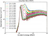 |
Fig. A.1. Simulated response function of the ERNE/HED penetrating-particle counter, accounting for both forward- and backward-penetrating protons. For the latter, the spacecraft structure below the instrument is assumed to correspond to an 10 cm thick aluminium layer. The different curves represent various (unknown) trigger levels of the bottom plastic scintillator in the stack. |
 |
Fig. A.2. Geometric factor (blue) and effective energy (red) of the penetrating-particle counter as a function of the plastic scintillator detection threshold (‘AC threshold’), obtained from bow-tie analysis. |
To better distinguish SEP events from other variations in the data (see Sect. 2.1), we also use a counter measuring particles that stop in the D3 detector (just above AC1), which is sensitive to protons in the ∼50–100 MeV range. An example time series of D3 and AC1 counters is shown in Fig. A.3. The algorithm scans the dataset using a 24-hour moving window advanced in three-hour steps. The first six hours of each window define the pre-event background, while the remaining 18 hours are searched for elevated count rates. If no enhancement is detected, the window is shifted forwards by three hours; if an event is found, it is advanced by nine hours to prevent double detections. Figure A.4 illustrates one example of detection (Event No. 166, 11 May 2024 01:50 UT). The red shading indicates the background interval, while the dashed and dotted lines show the mean background level μ and the upper level μd = μ + n ⋅ σ (with n = 5), respectively. Note that μd is not the detection threshold itself but limits the cumulative growth of the CUSUM function (see Huttunen-Heikinmaa et al. 2005). The data gaps in ERNE observations lasting seven days or longer are as follows:
-
25 February – 4 March 1997
-
24 June – 9 October 1998
-
14 – 21 November 1998
-
21 December 1998 – 8 February 1999
-
10 – 17 August 2001
-
5 – 12 February 2002
-
28 February – 11 March 2003
-
22 – 29 April 2004
-
26 November – 11 December 2006
-
29 July – 14 August 2009
-
7 – 24 September 2009
-
30 November 2011 – 5 January 2012
-
28 January – 10 February 2012
-
9 December 2012 – 31 January 2013
-
29 October – 4 December 2013.
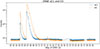 |
Fig. A.3. Example of ERNE counter observations (in counts per 5 minutes) from November 1997, showing two consecutive > 100 MeV proton events starting on 4 and 6 November, respectively. The AC1 counter corresponds to the penetrating-particle channel, while the D3 counter measures particles stopping near the bottom of the detector stack, i.e. those not triggering the plastic scintillator. |
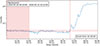 |
Fig. A.4. Detection of an event in the AC1 channel of SOHO/ERNE on 11 May 2024 01:50 UT. The pre-event background (red area) corresponds to the first six hours of the detection window. The dashed and dotted red lines indicate the background mean and the mean plus n times the standard deviation (n = 5), respectively. The vertical line marks the detected onset time. |
Some of the gaps listed by Paassilta et al. (2017) may contain short data intervals but are still treated as gaps for practical reasons, i.e. because meaningful event detection within them would not be possible. Since 2004, shorter and more frequent interruptions have also occurred, mainly due to the reduced telemetry rate of the SOHO spacecraft during so-called ‘keyhole periods’ (see Sect. 2.2), when the pointing of the high-gain antenna is suboptimal for communications.
Appendix B: SOHO/EPHIN high-energy protons data
EPHIN measures energetic particles – protons, electrons, and helium – across a wide range of energies, from a few mega-electronvolts up to several hundred mega-electronvolts (for details, see Müller-Mellin et al. 1995). The energy ranges for EPHIN are given in Kühl et al. (2020). As discussed in Kühl et al. (2015, 2016, 2017), the  –
– method can be applied to EPHIN’s integral channel to derive proton energy spectra from about 50 MeV to beyond 1 GeV. An extension of the EPHIN energy range for protons to above 1 GeV, based on energy-loss data from SSD A to D, has been implemented. Using extensive GEANT4 simulations of the instrument (Agostinelli et al. 2003), it has been shown that the initial energy of a proton penetrating EPHIN (i.e. triggering detectors A to F) can be inferred from the energy losses in SSD C and D. However, separating forward- and backward-penetrating protons is not possible, so the contribution from backward-penetrating particles must be accounted for. Due to the ageing of one of the thick SSDs, the method had to be adapted to use a thin SSD, namely SSD B.
B.1. Modification of the method by Kühl et al. (2015)
With SSD D becoming noisy in 2017, the method described by Kühl et al. (2015) could no longer be directly applied. As explained by Kühl et al. (2016), the energy resolution of the method depends on the energy-loss resolution of the SSDs involved. Thus, when using a total of 3300 μm instead of 8000 μm of silicon, a significant reduction in energy resolution is expected.
Figure B.1 shows the energy-loss-per-millimetre distributions of SSDs B (black), C (red), and D (green) during the 11 May 11 2024 (GLE74). The distribution for SSD D clearly deviates from the others, especially for  MeV/mm, where noise in SSD D strongly affects the signal. The right panel displays the minimum energy loss per millimetre obtained from SSDs C and D (black) and from SSDs C and B (red). Significant differences are found for
  MeV/mm. Figure B.2 compares the results of the method for two events reported by Kühl et al. (2015). The measurements agree well within the 50–200 MeV energy range and differ by less than 30% below 500 MeV, which is within the uncertainty estimated by Kühl et al. (2017). Another observation is the reduced energy resolution, as evident when compared to the spectra presented by Kühl et al. (2015).
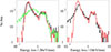 |
Fig. B.1.
|


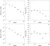 |
Fig. B.2. Proton energy-flux spectra from Kühl et al. (2015) (red symbols) and from this study (black symbols), and their corresponding differences (right panels). The upper and lower panels show the results using ten energy bins for GLE72 and for the sub-GLE event of 6 January 2014, respectively. |
B.2. Computation of the efficient energy and response for the > 100 MeV proton proxy
To estimate the > 100 MeV proton flux proxy, the energy range for protons from about 100 to 500 MeV needs to be covered to be comparable with the SOHO/ERNE channel (see Fig. A.1). As explained above, EPHIN utilises the dE/dx − dE/dx-method and relies on a precise assignment of the minimum of the two energy losses per path length in the two SSDs B and C (see Fig. B.3) to the incoming energy. Due to the stochastic processes of energy loss in matter, not a single incoming energy but a distribution of different particles may contribute to a single measured energy loss. We utilised the GEANT4 toolkit to compute the energy loss distributions for electrons in the energy range from 5 to 100 MeV and for protons and helium in the energy range from 50 MeV/amu to 2 GeV/amu (two times the rest mass of the particle), respectively. The runs were performed for particles with an energy distribution n(E) = n0 ⋅ Eγ and γ = −1 penetrating the instrument with an isotropic directional distribution. Since the determination of the response function is based on logarithmically spaced energy bins, γ = −1 leads to equal statistical uncertainties for each bin. Note that the influence of the power law index for SEP events is taken into account within the bow-tie method (see below).
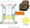 |
Fig. B.3. On the left and right a sketch and a photo of the EPHIN are shown, respectively. |
The helium-to-proton and electron-to-proton scaling was chosen 0.1 and arbitrarily, respectively. The latter takes into account the large variability of their relative intensities during SEP events (see e.g. Dresing et al. 2024). Figure B.4 shows the resulting contributions from electrons (green), protons (blue), and helium (orange).
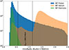 |
Fig. B.4. Contributions of electrons (green), protons (blue), and helium (orange) as functions of the minimum energy loss per path length in SSDs B and C, allowing for the minimisation of helium and electron contamination in the > 100 MeV integral proton channel (see text for details). |
For  MeV/mm (second vertical line in Fig. B.4), the distributions of sub-100 MeV protons and several-hundred-MeV/amu helium become ambiguous until
  MeV/mm, where helium dominates. At low
  , electrons and protons overlap: below 0.56 MeV/mm (first vertical line), measurements can be dominated by > 6 MeV electrons during SEP periods, while above 1.13 MeV/mm they can be influenced by relativistic helium during quiet times (Kühl et al. 2015, 2016, and references therein). The two vertical lines in the figure delimit the
  range selected for the > 100 MeV proton channel. Note, the contribution induced by helium does not vanish as expected. The reason for these entries is hadronic interactions in the spacecraft producing secondary protons and deuterium, respectively. Accordingly, the flux of > 100 MeV proton proxy is estimated using events with
  between 0.56 and 1.13 MeV/mm.
Utilising these energy loss limits the energy response of the > 100 MeV proton proxy was determined from the GEANT4 computations. The result is shown in the left panel of Fig. B.5. indicating that the proxy is primarily sensitive to protons with energies between about 120 and 450 MeV. The flux, Φ, can then be computed from the measured count rate, Csel, in the penetrating channel fulfilling the boundary condition
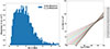 |
Fig. B.5. Left: Computed response function of the EPHIN > 100 MeV proton channel. The effective energy, Eeff, was determined using the bow-tie method (Oleynik 2021, Sect. 5.3.3) with power laws of spectral index between γ = 2 and γ = 5. Only the central response is considered to minimise instrumental effects occurring at high flux levels. |
by
 (B.1)
(B.1)
A bow-tie analysis, as described, for example, in Oleynik (2021), was applied to determine the effective energy Eeff and the corresponding integrated response function Reff. The method used here relies on the assumption that the incoming proton spectra are power-law spectra J(E, t) = J0 ⋅ Eγ with indices between −2 and −5. Utilising the energy response function shown in the left panel of Fig. B.5 allows us to obtain Eeff = 189 MeV and Reff = 60.34 cm2.sr.MeV. Note, Eeff obtained by EPHIN is somehow higher than the efficient energy from ERNE ranging between 128 and 172 MeV.
B.3. Fluence computation
Figure B.6 illustrates the computation of the fluence for GLE73, showing the > 100 MeV proton flux derived from EPHIN measurements. Vertical magenta lines mark the start and end times of the integration, while the horizontal magenta line indicates the selected background level.
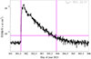 |
Fig. B.6. Example of fluence calculation from SOHO/EPHIN. The vertical magenta lines indicate the start and end times of the integration, while the horizontal line marks the background level used. |
B.4. Limitations
Figure B.7 shows two examples of limitations affecting the > 100 MeV proton channel derived from SOHO/EPHIN. The top panel illustrates the 1 October 2001 event, where data gaps result from limited telemetry and LELS issues, while the bottom panel shows the 20 September 2024 event, which occurred during a SOHO keyhole period. In both cases, the vertical line marks the ERNE-determined onset time. The black and red curves represent the hourly averaged flux of the > 100 MeV proton channel and the single-detector count rate of SSD F, respectively – the latter serving as a proxy for > 50 MeV protons, > 50 MeV/amu helium, and > 6 MeV electrons.
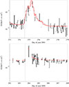 |
Fig. B.7. Top: Example of ‘low energy-loss statistics’ (LELS) during the 1 October 2001 event. Bottom: Example of a ‘keyhole period’ (KHP) on 20 September 2004. The black and red curves show the hourly averaged flux of the > 100 MeV proton channel and the single-detector count rate of SSD F, respectively. The vertical lines mark the onset times determined from ERNE data. |
Appendix C: Structure of the catalogue
-
Columns 1 and 2: identification of the event
-
Column 1: Catalogue entry number
-
Column 2: Event identifier
-
-
Columns 3 and 4: SOHO/ERNE data information
-
Column 3: Time of onset (in UT)
-
Column 4: Background mean of the channel [counts]
-
-
Columns 5 to 11: SOHO/EPHIN data information
-
Column 5: Background of the of > 100 MeV proton proxy channel [1/(cm2 sr s MeV)]
-
Column 6: Peak flux of the event [1/(cm2 sr s MeV)]
-
Column 7: Relative uncertainty on peak flux [%]
-
Column 8: Fluence of the event [1/(cm2 sr MeV)]
-
Column 9: Relative uncertainty on fluence [%]
-
Column 10: End time (for the integration) (in DOY)
-
Column 11: Comments
-
-
Columns 12 to 19: soft X-rays flare information
-
Column 12: Time of onset (in UT)
-
Column 13: Time of peak flux (in UT)
-
Column 14: Time of end (in UT)
-
Column 15: Soft X-ray class (1–8 Å soft X-ray peak intensity in terms of C, M and X nomenclature where these represent intensities of 10−6, 10−5, and 10−4 W/m2, respectively)
-
Column 16: Fluence [J/m2]
-
Column 17: X-ray location on the solar surface (in Stonyhurst heliographic co-ordinates, North (N) or South (S), and East (E) or West (W)) [degrees]
-
Column 18: Spacecraft observer
-
Column 19: Comments
-
-
Columns 20 to 28: hard X-ray flare information
-
Column 20: Time of onset (in UT)
-
Column 21: Time of peak flux (in UT)
-
Column 22: Time of end (in UT)
-
Column 23: Peak intensity [counts/s]
-
Column 24: Total counts [counts]
-
Column 25: Energy range [keV]
-
Column 26: Hard X-ray flare location on the solar surface (longitude, latitude in Carrington co-ordinates) [degrees]
-
Column 27: Spacecraft/instrument observer
-
Column 28: Comments
-
-
Columns 29 to 35: radio type III information
-
Column 29 to 31: Ground-based observations
-
Column 29: Ground-based station observer
-
Column 30: Onset time (in UT)
-
Column 31: Frequency range [MHz]
-
-
Column 32 to 34: Space-borne observations
-
Column 32: Spacecraft/instrument observer
-
Column 33: Onset time (in UT)
-
Column 34: Frequency range [kHz]
-
-
Column 35: Comments
-
-
Columns 36 to 42: radio type II information
-
Column 36 to 38: Ground-based observations
-
Column 36: Ground-based station observer
-
Column 37: Onset time (in UT)
-
Column 38: Frequency range [MHz]
-
-
Column 39 to 41: Space-borne observations
-
Column 39: Spacecraft/instrument observer
-
Column 40: Onset time (in UT)
-
Column 41: Frequency range [kHz]
-
-
Column 42: Comments
-
-
Columns 43 to 49: radio type IV information
-
Column 43 to 45: Ground-based observations
-
Column 43: Ground-based station observer
-
Column 44: Onset time (in UT)
-
Column 45: Frequency range [MHz]
-
-
Column 46 to 49: Space-borne observations
-
Column 46: Spacecraft/instrument observer
-
Column 47: Onset time (in UT)
-
Column 48: Duration [min]
-
Column 49: End frequency [MHz]
-
-
-
Columns 50 to 56: gamma-rays information
-
Column 50: Time of onset (in UT)
-
Column 51: Time of peak flux (in UT)
-
Column 52: Time of end (in UT)
-
Column 53: Peak intensity [counts/s]
-
Column 54: Total counts [counts]
-
Column 55: Spacecraft/instrument observer
-
Column 56: Comments
-
-
Columns 57 to 61: Coronal mass ejection information
-
Column 57: Time of first appearance (in UT)
-
Column 58: Linear speed [km/s]
-
Column 59: Space speed [km/s]
-
Column 60: Angular width [deg]
-
Column 61: Source of information
-
-
Column 62 to 65: GLE information
-
Column 62: GLE name
-
Column 63: Integral intensity [%.h]
-
Column 64: Omni-directional integral fluence [cm−2]
-
Column 65: Name of observer
-
-
Column 66: General notes
Appendix D: Solar associations timings distribution
Statistics on timing delays between SEP release times and their associated solar phenomena.
The most significant timing differences (> 360 minutes) correspond to the following SEP events (from largest to smallest):
-
Event 110 (6 March 2013, Δ(tSEP − tCME) = 1237 minutes), which presents a very slow rising phase
-
Event 114 (11 October 2013, Δ(tSEP − tCME) = 831 minutes), which also presents a very slow rising phase
-
Event 61 (8 November 2003, Δ(tSEP − tCME) = 831 minutes), for which only one strong far side CME occurring on the 7 November 2003 seems to be relevant. A more realistic onset could be hidden in the decay phase of the previous > 100 MeV proton event (number 60, 4 November 2003)
-
Event 89 (5 June 2011, Δ(tSEP − tCME) = 790 minutes), associated with a strong CME on the 4 June 2011 but which could also be related to a smaller one occurring at 08:00 UTC on 5 June 2011, enriched in high-energy SEPs due to the previous event
-
Event 76 (14 July 2005, Δ(tSEP − tCME) = 626 minutes), associated to a strong CME but alternatively related to two other smaller CMEs which occurred, respectively, six and seven hours after the first one
-
Event 124 (1 September 2014, Δ(tSEP − tCME) = 453 minutes)
-
Event 167 (13 May 2024, Δ(tSEP − tCME) = 452 minutes)
Appendix E: Radio instruments
Space-borne and ground-based instruments used in the search for radio burst associations with SEP events in the > 100 MeV proton catalogue, along with their corresponding frequency ranges and operational periods.
All Tables
Median and mean values with standard deviations (σ) of the parameters characterising the > 100 MeV proton events and the associated CMEs, soft and hard X-ray flares, and γ-ray emissions.
Statistics on timing delays between SEP release times and their associated solar phenomena.
Space-borne and ground-based instruments used in the search for radio burst associations with SEP events in the > 100 MeV proton catalogue, along with their corresponding frequency ranges and operational periods.
All Figures
|
Fig. 1. Temporal distribution of the > 100 MeV proton events included in the catalogue (histogram). Red dots show the corresponding peak proton intensities (Ip) with uncertainties measured by SOHO/EPHIN, plotted against the secondary (right-hand) axis. |
| In the text | |
|
Fig. 2. Distributions of > 100 MeV proton peak intensities (panel (a)) and fluences (panel (b)) measured by SOHO/EPHIN for 107 and 97 events of the catalogue, respectively. |
| In the text | |
|
Fig. 3. Representative example of the solar associations for the 28 October 2021 > 100 MeV SEP event (No 137) corresponding to GLE73. Panel (a): ERNE proton counts at > 100 MeV. Panel (b): Soft X-ray flux (1–8 Å, GOES, blue) and high-energy flare emissions, including hard X-rays (Solar Orbiter/STIX, 4–10 keV, purple) and γ-rays (Fermi/LAT, > 100 MeV flux, pink). Panel (c): Radio dynamic spectrum (e.g. Wind/WAVES) with over-plotted CME height–time profile from coronagraph observations (SOHO/LASCO). Panel (d): Ground-level neutron monitor data showing relativistic particle increases. |
| In the text | |
|
Fig. 4. Statistics of the identified soft X-ray flares associated with > 100 MeV SEP events (131/172, 76%). From left to right: SXR peak flux, flare longitude in Stonyhurst co-ordinates, rise time (peak minus start time), and total duration. |
| In the text | |
|
Fig. 5. Statistics of the identified hard X-ray flaring sources for the > 100 MeV catalogue (76%, 131/172 events). From left to right: distribution of HXR peak intensity, flare fluence (in counts), rise time (HXR peak – start), and total duration. |
| In the text | |
|
Fig. 6. Statistics on the CMEs associated with the > 100 MeV events (96%, 162/169 events). Panel (a): CME speed distribution (kilometre per second). Panel (b): CME width distribution (deg). |
| In the text | |
|
Fig. 7. Distribution of the SEP events with respect to timing differences (in minutes) between the > 100 MeV proton events release times determined with SOHO/ERNE SEP onset and the associated solar signatures onsets. Two travel-time assumptions are considered: short (light colours) and long (dark colours) path lengths, respectively, 1 and 2.5 AU. Solar signatures are shifted to the solar time according to the light travel time, and are, from left to right: CME first appearance in SOHO/LASCO coronographs (blue), soft X-ray onset time (red), hard X-ray onset time (yellow), type II radio burst onset time (purple), type III radio burst onset time (green), type IV radio burst onset time (cyan), gamma ray burst onset time (pink). In each boxplot, the middle line indicates the median of the distribution whereas the top of bottom edges of a box are the upper and lower quartiles, respectively. Outliers are values that are more than 1.5 times the distance between the top and bottom edges. The number of events considered in each boxplot is indicated in the x axis. |
| In the text | |
|
Fig. 8. Same as Figure 7 for the timing difference between solar associations in minutes. From left to right, comparisons between: soft X-ray onset time (tSXR) and CME first appearance in SOHO/LASCO coronographs (tCME) (blue) ; tCME and type II radio burst onset time (ttII) (red) ; tSXR and type III radio burst onset time (ttIII) (yellow) ; tSXR and type IV radio burst onset time (ttIV) (purple) ; tSXR and gamma ray burst onset time (tγ) (green) ; ttIII and ttIV (cyan) ; ttIII and ttII (pink). |
| In the text | |
|
Fig. 9. Timing difference (hours in UT) between soft and hard X-rays. |
| In the text | |
|
Fig. 10. Hard X-ray peak intensity in counts/s from RHESSI (red points) and Solar orbiter/STIX (blue points) as a function of soft X-ray peak intensity in W/m2 from GOES. The PCC of the respective best fits (red and blue lines) are indicated in the legend. |
| In the text | |
|
Fig. 11. Coronal mass ejection speed from SOHO/LASCO as a function of the soft X-ray peak from GOES, for 49 events studied in Salas-Matamoros & Klein (2015) (grey), 65 SEP events that reach E > 100 MeV studied by Papaioannou et al. (2023) (blue), and 124 events from the present catalogue (orange). Power law fits for our sample and the combined three are lines in orange and pink, respectively. |
| In the text | |
|
Fig. 12. SOHO/EPHIN proton peak intensity > 100 MeV (Ip) with uncertainties as a function of the soft X-ray peak from GOES. Events considered as well connected, i.e with a SXR longitude between 20 and 87 degrees, are shown in pink. Pearson correlation coefficients of well-connected and all events are, respectively, in pink and black. |
| In the text | |
|
Fig. 13. SOHO/EPHIN proton peak intensity > 100 MeV (Ip) with uncertainties as a function of the linear CME speed measured with SOHO/LASCO (VCME). |
| In the text | |
|
Fig. 14. SOHO/EPHIN proton peak intensity > 100 MeV (Ip) with uncertainties as a function of the integral GLE peak intensity (%.h) for 14 events of the present catalogue. |
| In the text | |
|
Fig. 15. SOHO/EPHIN proton fluence with uncertainties as a function of the omnidirectional integral GLE fluence expressed in cm−2 for 10 events of the present catalogue. |
| In the text | |
|
Fig. A.1. Simulated response function of the ERNE/HED penetrating-particle counter, accounting for both forward- and backward-penetrating protons. For the latter, the spacecraft structure below the instrument is assumed to correspond to an 10 cm thick aluminium layer. The different curves represent various (unknown) trigger levels of the bottom plastic scintillator in the stack. |
| In the text | |
|
Fig. A.2. Geometric factor (blue) and effective energy (red) of the penetrating-particle counter as a function of the plastic scintillator detection threshold (‘AC threshold’), obtained from bow-tie analysis. |
| In the text | |
|
Fig. A.3. Example of ERNE counter observations (in counts per 5 minutes) from November 1997, showing two consecutive > 100 MeV proton events starting on 4 and 6 November, respectively. The AC1 counter corresponds to the penetrating-particle channel, while the D3 counter measures particles stopping near the bottom of the detector stack, i.e. those not triggering the plastic scintillator. |
| In the text | |
|
Fig. A.4. Detection of an event in the AC1 channel of SOHO/ERNE on 11 May 2024 01:50 UT. The pre-event background (red area) corresponds to the first six hours of the detection window. The dashed and dotted red lines indicate the background mean and the mean plus n times the standard deviation (n = 5), respectively. The vertical line marks the detected onset time. |
| In the text | |
|
Fig. B.1.
|
| In the text | |
|
Fig. B.2. Proton energy-flux spectra from Kühl et al. (2015) (red symbols) and from this study (black symbols), and their corresponding differences (right panels). The upper and lower panels show the results using ten energy bins for GLE72 and for the sub-GLE event of 6 January 2014, respectively. |
| In the text | |
|
Fig. B.3. On the left and right a sketch and a photo of the EPHIN are shown, respectively. |
| In the text | |
|
Fig. B.4. Contributions of electrons (green), protons (blue), and helium (orange) as functions of the minimum energy loss per path length in SSDs B and C, allowing for the minimisation of helium and electron contamination in the > 100 MeV integral proton channel (see text for details). |
| In the text | |
|
Fig. B.5. Left: Computed response function of the EPHIN > 100 MeV proton channel. The effective energy, Eeff, was determined using the bow-tie method (Oleynik 2021, Sect. 5.3.3) with power laws of spectral index between γ = 2 and γ = 5. Only the central response is considered to minimise instrumental effects occurring at high flux levels. |
| In the text | |
|
Fig. B.6. Example of fluence calculation from SOHO/EPHIN. The vertical magenta lines indicate the start and end times of the integration, while the horizontal line marks the background level used. |
| In the text | |
|
Fig. B.7. Top: Example of ‘low energy-loss statistics’ (LELS) during the 1 October 2001 event. Bottom: Example of a ‘keyhole period’ (KHP) on 20 September 2004. The black and red curves show the hourly averaged flux of the > 100 MeV proton channel and the single-detector count rate of SSD F, respectively. The vertical lines mark the onset times determined from ERNE data. |
| In the text | |
Current usage metrics show cumulative count of Article Views (full-text article views including HTML views, PDF and ePub downloads, according to the available data) and Abstracts Views on Vision4Press platform.
Data correspond to usage on the plateform after 2015. The current usage metrics is available 48-96 hours after online publication and is updated daily on week days.
Initial download of the metrics may take a while.